Classical, Evolutionary, and Deep Learning Approaches of Automated Heart Disease Prediction: A Case Study

Abstract

Cardiovascular diseases (CVDs) are the leading cause of death globally. Detecting this kind of disease represents the principal concern of many scientists, and techniques belonging to various fields have been developed to attain accurate predictions. The aim of the paper is to investigate the potential of the classical, evolutionary, and deep learning-based methods to diagnose CVDs and to introduce a couple of complex hybrid techniques that combine hyper-parameter optimization algorithms with two of the most successful classification procedures: support vector machines (SVMs) and Long Short-Term Memory (LSTM) neural networks. The resulting algorithms were tested on two public datasets: the data recorded by the Cleveland Clinic Foundation for Heart Disease together with its extension Statlog, two of the most significant medical databases used in automated prediction. A long series of simulations were performed to assess the accuracy of the analyzed methods. In our experiments, we used F1 score and MSE (mean squared error) to compare the performance of the algorithms. The experimentally established results together with theoretical consideration prove that the proposed methods outperform both the standard ones and the considered statistical methods. We have developed improvements to the best-performing algorithms that further increase the quality of their results, being a useful tool for assisting the professionals in diagnosing CVDs in early stages.

1. Introduction

Cardiovascular diseases (CVDs) are one of the main causes of the rising mortality rate all around the world, with an unhealthy diet, alcohol consumption, smoking, and a lack of physical activity contributing to the risk of developing such conditions. CVDs are a class of disorders of the heart and blood vessels mainly consisting of coronary heart, cerebrovascular, and rheumatic heart disease, respectively. CVDs take an estimated 17.9 million lives each year, which is an estimated 32% of all deaths worldwide [1]. As symptoms can often be similar to those of other illnesses and age-related issues, it is difficult for medical professionals to diagnose them. Finding the people at highest risk of CVDs, early diagnosis and appropriately treating those suffering from this kind of disease can prevent premature deaths.

Detecting CVDs represents the principal concern of many scientists in the artificial intelligence area, and various techniques have been developed for attaining a method that can perform this accurately, such as classical statistical strategies, machine learning, deep learning-oriented algorithms, and evolutionary computation-based mechanisms together with various data mining pre-processing methods.

The paper focuses on the diagnosis of cardiovascular diseases through three types of classification methods: classical approaches, LSTM-based algorithms, and hybrid techniques. The resulting algorithms were tested to diagnose CVDs using the data recorded by Cleveland Clinic Foundation [2,3] together with its extension Statlog [4].

The traditional approaches to the dichotomic classification problem used in this paper are random forest, KNN, logistic regression, and SVM methods. We also used LSTM-based algorithms, and following our study, we have chosen the most promising methods for hybridization, namely, SVM and stacked LSTM.

The main contribution of this paper is the development of two complex hybrid methods that combine hyper-parameters optimization methods with the SVM approach and stacked LSTM architecture to improve diagnostic accuracy. In our work, we use a two-membered evolution strategy and a fitness function defined based on the classifier’s hyper-parameters to improve the accuracy of the SVM algorithm, and we used a TPE-based optimization to obtain a more accurate LSTM diagnosis system. A long series of simulations were performed to assess the accuracy of the results. The experimentally established results together with theoretical considerations prove that the new methods outperform both the standard ones and the considered statistical methods.

The rest of the paper is organized as follows. A brief review of some state-of-the-art papers dealing with automated CVD diagnostic systems and various datasets recording medical information is provided in Section 2. Section 3 presents a series of classification algorithms commonly used to identify CVDs, according to the above-mentioned state-of-the-art literature review. Section 4 is the core of our research work, and it introduces the hybrid classification approaches. The experiments proving the effectiveness and the performances of the proposed algorithm against standard methods are provided in Section 5. The concluding remarks and ideas for future developments are reported in the final section of the paper.

2. Related Work

2.1. Classical ML Techniques

In [5], three different approaches based on classical statistical methods were used to identify CVDs. The first approach is based on the usage of various machine learning (ML) algorithms, such as random forest, logistic regression, K-Nearest Neighbors (KNN), support vector machine (SVM), decision tree, and XGBoost, using the UCI Heart Disease dataset. Note that feature selection and outliers detection were not considered. The second approach used only the feature selection mechanism, while the third approach brought both feature selection and outliers detection into practice. The most accurate algorithm was obtained in the last approach by KNN, with the percentage of correct classification being 84.86%.

The research reported in [6] also uses statistical models such as SVM, Gaussian Naïve Bayes (GNB), logistic regression, LightGBM, CGBoost, and random forest (RF) to create a classifier that is tested and trained on the Cleveland Clinic Foundation for Heart Disease dataset. The accuracy of the models is measured using performance matrices and confusion matrices. The experimentally established results pointed out that the random forest classifier achieved the best accuracy, followed by SVM and logistic regression.

Various ML techniques, including SVMs, decision trees (DTs), and Naïve Bayes (NB), were used in [7] to generate diagnosis results on the South African Heart Disease dataset. The performance of these models was compared according to accuracy, sensitivity, specificity, true positives (TPs), true negatives (TNs), false positives (FPs), and false negatives (FNs). Results indicated that NB had the highest accuracy rate; however, it was not satisfactory in terms of specificity and sensitivity. On the contrary, SVMs and DTs provided higher specificity ratings but displayed inadequate sensitivity. Thus, it was concluded that further research is necessary to elevate the performance and increase sensitivity and specificity scores.

Additionally, the research work reported in [8] has demonstrated the efficacy of using a cost-sensitive ensemble method for the diagnosis of heart diseases. To assess the performance of this approach, the Statlog, Cleveland, and Hungarian heart disease datasets were selected for analysis. Furthermore, various metrics, such as E, MC, G-mean, precision, recall, specificity, and AUC, were used to measure the effectiveness of the classifiers. Relief algorithms were employed to identify the most pertinent features and eliminate any effects of irrelevant features. This study has provided promising results and is a step forward in the development of more sophisticated classifiers with improved accuracy when used in combination with new algorithms.

Recent research has demonstrated the utility of ML techniques in forecasting the 90-day prognosis of individuals diagnosed with transient ischemic attack and minor stroke. The study, conducted in [9], utilized data from the CNSR-III prospective registry study, which included demographic, physiological, and medical history information of patients with the medical condition. The authors found that models constructed using logistic regression and machine learning exhibited superior performance, as evidenced by their Area Under the Curve (AUC) measure exceeding 0.8. Of the models employed, the Catboost model demonstrated the highest AUC score at 0.839.

2.2. Deep Learning Techniques

With the development of computing power appeared the chance to use more resource demanding algorithms, which are a subcategory of machine learning models named deep learning (DL). Those algorithms have evolved rapidly in recent years and have proven useful, with robust results for various projects, in different areas of interest.

Diagnosing diseases is a good example of showcasing the abilities of deep learning models and the different areas they excel in classification problems. In [10], the possibility of categorizing and understanding MRI scans to diagnose brain tumors is studied. By comparing two models, the convolutional neural networks (CNN) and a deep neural network (DNN), which is typically a feed-forward network and makes it a perfect fit for these types of problems, it is concluded that the latter provides the most accurate results.

The authors of [11] proposed the usage of multiple data mining and deep learning techniques, using a dataset containing information selected by taking into account the history of patients’ heart problems in correlation with other medical aspects. Experimentally established results showed that the best classification scores of the proposed ML approach were obtained by the random forest classifier: accuracy (90.21%), precision (90.22%), recall (90.21%), and F1 score (90.21%).

In [12], a CNN-based diagnosis system was proposed. This model was found to be comparably effective to traditional machine learning models, such as SVM and random forests, particularly in predicting negative cases, meaning those cases without coronary heart disease. The architecture of the proposed model was a sequential feedforward one-input–one-output network, which begins with the application of LASSO regression, which adds a penalty and eliminates coefficients that help control true negatives in the dataset.

There has been research that used both machine and deep learning algorithmic approaches to classify and create predictions for heart diseases. It has been proven that taking into account the medical history of the patients allows deep learning models to outperform machine learning algorithms and yield high accuracy [11].

2.3. Hybrid Methods

A hybrid method aiming to extract significant features using ML techniques for CVDs prediction was reported in [13]. The classification model was developed with various feature combinations and is based on the aggregation of random forest and linear classification models. The proposed algorithm, hybrid random forest with a linear model (HRFLM), was assessed to have an 88.7% accuracy. The study also points to the idea that new feature selection methods and new combinations of ML techniques can be used to achieve highly accurate classification algorithms.

Another method to classify patients suffering from CVDs is reported in [14]. The method is based on the usage of ML techniques and ontology to build an efficient model capable of accurately predicting the presence of cardiac disease and facilitating early diagnosis. The main purpose is to extract the relevant rules from the DT algorithm, then to implement these rules in an ontology using the Semantic Web Rule Language (SWRL). The model reached a level of accuracy of 75% and an F1 score of 80.5%, outperforming the standard DT model (73.1% accuracy, 73.8% F1 score).

In the case study presented in [15], the usage of evolutionary algorithms (EAs), such as genetic algorithms (GAs) and particle swarm optimization (PSO), was proved to raise the overall accuracy of ML algorithms. The reported research combines EAs with Naïve Bayes and support vector machine for feature selection. The most successful algorithm in terms of classification accuracy uses GA as a feature extraction strategy.

Various techniques can be used to enhance deep learning algorithms to increase their accuracy. An example is the combination of a Multilayer Perceptron (MLP) algorithm with the use of the Back Propagation of Errors Algorithm, which fine tunes the weights based on the error rate acquired from the previous iteration [16]. It was experimentally proved that the new model has improved performance compared to similar approaches, thus creating a better tuned MLP model for the use of classification problems.

Another way to optimize the algorithms is to use swarm intelligence optimization techniques. Such a technique is particle swarm optimization (PSO) which helps the model to determine the optimal weight and bias values. Combining this technique with a MLP model and testing on the heart disease dataset gives a model that outperformed the initial model [17].

In [18], various techniques for recognizing cardiovascular diseases (CVDs) were examined, including Data Mining (DM), DL, ML, and Soft Computing. The authors reviewed the literature on CVD recognition and presented the findings in terms of advantages, limitations, and accuracy levels. The results revealed that certain approaches, such as the utilization of DM and GAs, yielded high accuracy scores of around 96%. However, other methods produced lower accuracy levels, with accuracy scores of around 45%. The best accuracy was observed in the use of Neural Networks (NN), which achieved a score of 99%.

The capabilities of different methods in predicting heart disease can be further enhanced by analyzing the data obtained from other sources such as electrocardiograms (ECGs). ECG waves are widely used to diagnose cardiovascular illnesses. The work reported in [19] aims to develop a non-linear vector decomposed neural network (NVDN) to classify ECG data. The proposed method was tested using well-known datasets from UCI and Physio net. After denoising the images with the use of frequency wavelet decay strategies, a subset of common features is identified. The NVDN model is then used to predict CVDs. The model produces decent results in terms of the F1 score, accuracy, sensitivity, and specificity; however, the forecasts are inaccurate. It is thus proposed to minimize time complexity and improve categorization.

In [20], neuro-fuzzy systems were used to learn predictive models from training data to create decision rules meant to support the decision-making process in cardiovascular risk assessment. The reported accuracy has reached 0.91, proving that artificial intelligence models are a valuable help for clinicians.

The literature review shows that there are many possibilities and opportunities for optimization techniques and different approaches to improve the accuracy of the deep learning models, which makes them even better candidates for classification problems.

Recent studies aiming to increase the accuracy of the diagnosis systems indicate that hyperparameter optimization techniques proved powerful tools. In [21], a radial basis function neural network (RBFNN) designed to identify and diagnose non-linear systems is proposed. The hyperparameters of the RBFNN are computed using PSO-based techniques. The resulting algorithm, which incorporates a spiral search mechanism, proves to improve prediction accuracy and can be extended to various types of neural networks. A PSO algorithm is also used for parameter optimization in [22]. The proposed diagnostic system is based on CNN and recognizes malignant and benign people in the attempt of identifying early-stage breast cancer.

A novel ensemble technique combining NB, DT, and SVM is introduced in [23] to classify heart diseases. The proposed approach involves two layers of base learners and a final meta-learner used to optimize the prediction accuracy. Other approaches involving a more accurate representation of neuronal activity use spiking neural networks [24]. To optimize the recognition rate, various heuristic algorithms including Cuckoo Search Algorithm, Grasshopper Optimization Algorithm, and Polar Bears Algorithm are used to compute the parameters of the spiking NN.

3. Standard Binary Classification Algorithms

3.1. The Dichotomic Classification Problem

Let $\mathcal{S}=\left\{\left(x_i,y_i\right), x_i\in {ℝ}^n,y_i\in \left\{-1,1\right\},1\le i\le N\right\}$ be a finite set of labeled examples coming from two classes, denoted by $h_1$ and $h_2$. The main task of binary classification (recognition) problems is to predict based on $\mathcal{S}$ if a test sample belongs to one of $h_1$ or $h_2$, or if its corresponding class cannot be determined. For each $i, 1\le i\le N$, $x_i$ is a particular example, and $y_i$ represents the label of the provenance class of $x_i$. The examples coming from $h_1$ are conventionally labeled by 1, while those belonging to $h_2$ are conventionally labeled by −1. Consequently, the elements of $h_1$ are referred to as the positive samples, and the components of $h_2$ are the negative ones.

The most commonly used classifiers are of parametric type. The decision function inputs are a finite set of parameters and samples. Special attention is given to the linear classifiers, due to their simplicity. The classification decision is based on a linear combination of inputs $h_{w,b}:{ℝ}^n\to \left\{-1, 1\right\}$,

$$h_{w,b}\left(x\right)=\left\{\begin{array}{cc}1,& w^T·x+b\ge 0 \\ -1,& w^T·x+b<0\end{array}\right.,$$

(1)

having the parameters $w\in {ℝ}^n$ and $b\in ℝ$. The set $\mathcal{S}$ is linearly separable if there exists a pair $\left(w,b\right)$ such that the hyperplane $h_{w,b}$ separates the two classes, that is

$${\mathcal{H}}_{\mathcal{S}}=\left\{\left(w,b\right)\left|w\in {ℝ}^n,b\in ℝ,\left(w^T{x}_i+b\right)y_i>0, \left(x_i,y_i\right)\in \mathcal{S}\right.\right\}\ne \varnothing ,$$

(2)

Note that, in most real-world problems, it is difficult to verify whether $\mathcal{S}$ is linearly separable. Additionally, even if the linear separability is assumed, the parameters (w, b) may be unknown or their computation may be un-tractable. In such cases, the classification can be performed in a so-called feature space $\mathcal{F}$, in the hope that the image of $\mathcal{S}$ in $\mathcal{F}$ is a linearly separable set or at least its separability degree is increased. The projection of $\mathcal{S}$ onto $\mathcal{F}$, ${\mathcal{S}}_g=\left\{\left(g\left(x_i\right),y_i\right), x_i\in {ℝ}^n,y_i\in \left\{-1,1\right\},1\le i\le N\right\}$, is of non-linear type, and it is defined by a vector valued function $g:{ℝ}^n\to \mathcal{F}$, called a feature extractor. The classification problem is translated to $\mathcal{F}$ and consists of the computation of the decision function

$$h_{b,w}\left(x\right)=\left\{\begin{array}{cc}1,& w^{T}g\left(x\right)+b\ge 0\\ -1,& w^{T}g\left(x\right)+b<0\end{array}\right.,$$

(3)

where $w\in \mathcal{F}$, and $b\in ℝ$.

From the practical point of view, one has to select a function K that covers the functional expression of $g$ to allow the computation of $\left(w^{T}g\left(x\right)+b\right)$ [25].

If $\mathcal{S}$ is not known to be linearly separable, the linear classifiers, even those designed to minimize the classification error, can fail to provide accurate results. In such cases, non-linear classifiers can be considered instead. One of the most successful models of non-linear classifiers used in medical diagnosis is DNNs.

Note that in parametric classification, that data is assumed to be drawn from one or a mixture of known probability distributions. The non-parametric approaches are used when no such assumption can be made, and “the data speaks for itself” [26]. The most commonly used non-parametric classifiers applied in automated medical diagnosing are the KNN-, DT-, and RF-based methods, respectively.

3.2. Logistic Regression Classifier

Standard logistic regression is a dichotomic linear classifier that deals with categorical data, and it is widely used in analyzing medical data. The basic method is applied to linearly separable sets, but it can be extended to classify non-separable data using kernel functions [27,28].

We denote by $\beta \in {ℝ}^n$, ${\beta }_0\in ℝ$ the model parameters. Linear logistic regression is based on the posterior probability of each class, $P\left(Y|x;\beta ,{\beta }_0\right)$. The probability of a positive example is $P\left(Y=1|X=x;\beta ,{\beta }_0\right)$. The expression $\frac{P\left(Y=1|X=x;\beta ,{\beta }_0\right) }{1-P\left(Y=1|X=x;\beta ,{\beta }_0\right) }$ defines the odds ratio. The logistic model considers the log-odds as a linear function, that is, denoting $P\left(Y=1|X=x;\beta ,{\beta }_0\right)$ by $p\left(x;\beta ,{\beta }_0\right)$, the logistic function for $p\left(x;\beta ,{\beta }_0\right)$ is defined by

$$logit\left(p\left(x;\beta ,{\beta }_0\right)\right)=log\left(\frac{p\left(x;\beta ,{\beta }_0\right)}{1-p\left(x;\beta ,{\beta }_0\right)}\right)={\beta }^T·x+{\beta }_0,$$

(4)

Using straightforward computation, from Equation (4), we obtain

$$p\left(x;\beta ,{\beta }_0\right)=\sigma \left({\beta }^T·x+{\beta }_0\right),$$

(5)

where $\sigma \left(·\right)$ is the logistic sigmoid function defined by

$$\sigma \left(z\right)=\frac{1}{1+exp\left(-z\right)},$$

(6)

The classifier is developed based on the idea that $p\left(x;\beta ,{\beta }_0\right)$ should be close to 1 for positive data, and close to 0 for negative examples. One of the most popular ways to compute the estimates $\widehat{\beta },\widehat{{\beta }_0}$ is the maximum likelihood method. [29]

3.3. K-Nearest Neighbors Classifier

The KNN algorithm is a non-parametric ML technique which makes no assumptions regarding the available dataset $\mathcal{S}$. The idea underlying this technique is that similarity means closeness. KNN classifies new instances based on the closest k training samples in $\mathcal{S}$, where the closeness is expressed in terms of a distance function [30]. In most approaches, Euclidian distance is used to implement the KNN method.

Being given a certain input data $x_{new}$, the algorithm computes the closest k elements in $\mathcal{S}$ to $x_{new}$ and classifies $x_{new}$ based on the classes of these neighbors. The accuracy of KNN depends on k and the data dimension. The algorithm does not involve an actual training phase. On the other hand, every time new example $x_{new}$ has to be classified, the distances between $x_{new}$ and every member of $\mathcal{S}$ must be computed [26].

3.4. Decision Trees and Random Forests

Decision trees are non-parametric, supervised learning methods, implementing the divide-and-conquer strategy. A decision tree is a hierarchical model consisting of internal decision nodes and terminal leaves. Each internal node t corresponds to a discrete-valued decision function $f_t\left(·\right)$ that labels the branches. The function $f_t\left(·\right)$ is a discriminant in the input space, dividing it into smaller regions. In case of classification DTs, each leaf node is associated with a class label and defines a specific region in the input space. An example x is processed recursively starting with the root, until a leaf node is reached. At each internal node, a test is applied, and one of the branches is selected based on the response. The example x is classified according to the output label of the obtained leaf node.

An input dataset $\mathcal{S}$ can be correctly encoded by many classification DTs; therefore, the aim is to compute the “smallest” one. The size of a DT is measured in terms of the number of nodes and the complexity of the decision functions associated with the internal nodes.

The standard DT learning algorithm is of greedy type. It starts with the root associated with $\mathcal{S}$ and, at each step, recursively looks for the best split of the current input set, until no more splits are needed and a leaf node is created and labeled.

The quality of a split is computed based on an impurity measure. A split is said to be pure if, for all resulted branches, all the instances choosing a branch belong to the same class h. If a split is pure, the procedure is over, and a leaf node labeled with h is added. Otherwise, the instances should be split to minimize the impurity of the results. The most commonly used impurity measures are the entropy (7), Gini index (8) and the misclassification error (9).

$$\phi \left(p,1-p\right)=-p·{\log }_{2}p-\left(1-p\right)·{\log }_2\left(1-p\right),$$

(7)

$$\phi \left(p,1-p\right)=2·p·\left(1-p\right),$$

(8)

$$\phi \left(p,1-p\right)=1-\underset{}{\max }\left(p,1-p\right),$$

(9)

where $p$ is the probability of the positive class.

DTs are very popular due to the classification speed and interpretability (easy to described as a set of IF-THEN rules). For these reasons, sometimes they are preferred instead of other harder-to-interpret methods.

Using more than one DT can lead to significant improvement of classification accuracy. Thus, the idea of RF algorithm was born. RF is an ensemble of DTs, each one being created from a randomly selected subset of $\mathcal{S}$, using a random subset of features at each decision node to diversify the individual classifiers. In order to classify a new example, it is put through all the trees in the forest. The outcome of each tree represents a vote and the final result is decided accordingly. In the particular case of medical diagnosis, the dimension of the input is usually large, and each attribute contains a small piece of information. This kind of problems benefits from the use of RF instead of a single DT [31].

3.5. SVM Classifiers

Pattern recognition techniques seek to minimize a criterion in order to optimize the accuracy. The traditional methods focus on minimizing the empirical risk. Opposed to them, SVMs focus on the structural risk, which means the probability of outputting the wrong classification of new examples [25,32]. Many real-world applications involving high dimension datasets have benefited from the SVMs, due to their powerful generalization capability. One such field is automated medical diagnosis.

3.5.1. Linear SVMs

The simplest SVM model defines a linear separating hyperplane that determines a maximum margin classifier. The best generalization capability, which means new examples are correctly classified, requires the computation of the optimal margin classifier $\left(w^{\ast },b^{\ast }\right)\in {\mathcal{H}}_{\mathcal{S}}$ that separates the training samples with the largest “gap”. Mathematically, an optimal margin classifier is a solution of the quadratic programming (QP) problem

$$\left\{\begin{array}{l}\mathrm{minimize}\frac{1}{2}{||w||}^2\\ y_i\left(w^T{x}_i+b\right)\ge 1,\hspace{1em}1\le i\le N\end{array}\right.,$$

(10)

One way to solve problem (10) is to apply the Lagrange multiplier method. The dual optimization problem is defined by

$$\left\{\begin{array}{l}\mathrm{maximize}{\displaystyle \sum _{i=1}^N}{\alpha }_i-\frac{1}{2}{\displaystyle \sum _{i=1}^N}{\displaystyle \sum _{j=1}^N}{\alpha }_i{\alpha }_j{y}_i{y}_j{x}_i{}^T{x}_j\\ {\displaystyle \sum _{i=1}^N}{\alpha }_i{y}_i=0\\ {\alpha }_i\ge 0,1\le i\le N\end{array},\right.$$

(11)

The optimal value of w is [29]

$$w^{\ast }={\displaystyle \sum _{i=1}^N}{\alpha }_i^{\ast }{y}_i{x}_i$$

(12)

where ${\alpha }^{\ast }={\left({\alpha }_1{}^{\ast },{\alpha }_2{}^{\ast },\dots ,{\alpha }_N{}^{\ast }\right)}^T$ is a solution of Equation (11).

The parameter b is not unique and cannot be computed by solving the problem (10). One of the usual choices for b is [25]

$$b^{\ast }=-\frac{1}{2}\left\{\underset{\begin{array}{l}i\\ y_i=-1\end{array}}{max}{w}^{\ast T}{x}_i+\underset{\begin{array}{l}i\\ y_i=1\end{array}}{min}{w}^{\ast T}{x}_i\right\}.$$

(13)

3.5.2. Non-Linear SVMs

In more complex cases, when $\mathcal{S}$ is not known to be linearly separable, the first approach is to map the original input space into a feature space by using non-linear transformations $g$, hoping that ${\mathcal{S}}_g$ is linearly separable. A series of kernel functions have been extensively used in the published literature, most successful being radial-based functions (RBF), for instance, Gaussian RBF and Exponential RBF [25,33].

If K is a kernel function covering the feature extractor g, similar to Section 3.5.1, an optimal margin classifier corresponds to $\left(w^{\ast },b^{\ast }\right)$, where [32]

$$w^{\ast }={\displaystyle \sum }_{i=1}^N{\propto }_i^{\ast }{y}_{i}g\left(x_i\right),$$

(14)

$$b^{\ast }=-\frac{1}{2}\left\{\underset{i,y_i=-1}{\max }{\displaystyle \sum }_{j=1}^N{\propto }_j^{\ast }{y}_{j}K\left(x_j,x_i\right)+\underset{i,y_i=1}{\min }{\displaystyle \sum }_{j=1}^N{\propto }_j^{\ast }{y}_{j}K\left(x_j,x_i\right)\right\}$$

(15)

Note that the optimal separating hyperplane is defined in terms of the kernel function K, the vector ${\alpha }^{\ast }$ and the elements of $\mathcal{S}$ [34].

In our work we used the Gaussian RBF kernel, defined by

$$K\left(x, y\right)=e^{-\gamma {\left|\left|x-y\right|\right|}^2}$$

(16)

3.5.3. Non-Linear Soft-Margin SVMs

If the feature extractor g fails to produce a linearly separable dataset, the second approach is to seek a $\left(w,b\right)$ that “mimics” as closely as possible the behavior of $\mathcal{S}$. For this, the non-linear SVM is extended by including the slack variables ${\xi }_1,{\xi }_2,\dots ,{\xi }_N$. Each ${\xi }_i$ represents the magnitude of the classification error corresponding to the observation $\left(x_i,y_i\right)$

$${\xi }_i=max\left\{0,1-y_i\left(w^{T}g\left(x_i\right)+b\right)\right\}$$

(17)

The obtained model is called soft-margin SVM.

The cumulated error is usually defined by a convex and monotonically increasing function F

$$F\left({\displaystyle \sum }_{i=1}^N{\xi }_i^t\right)$$

(18)

where $t>0$. The simplest model uses $F\left(u\right)=u$ and $t=1$, and therefore, the SVM problem is given by [26]

$$\left\{\begin{array}{l}minimize \left\{\frac{1}{2}{||w||}^2+C{\displaystyle \sum _{i=1}^N}{\xi }_i\right\}\\ y_i\left(w^{T}g\left(x_i\right)+b\right)\ge 1-{\xi }_i, 1\le i\le N \\ {\xi }_i\ge 0, 1\le i\le N\end{array}\right.$$

(19)

where C is a weight parameter that expresses the effect of the cumulated error.

Similarly to Section 3.5.2, if ${\propto }^{\ast }={\left({\propto }_1^{\ast },{\propto }_2^{\ast },\dots ,{\propto }_N^{\ast }\right)}^T$ is a solution of the QP-dual problem corresponding to Equation (19), then the parameters $\left(w^{\ast },b^{\ast }\right)$ are given by Equations (14) and (15). Note that the constraints of the dual problem are $0\le {\propto }_i\le C, 1\le i\le N$.

3.6. DNN Classifiers

The classifiers designed using DNN models are among the most successful automated medical diagnose procedures. The study of the state-of-the-art literature leads to the conclusion that the most promising architectures are based on CNNs and RNNs. The LSTM architecture is a subcategory of RNNs that has demonstrated high classification accuracy.

3.6.1. CNN

The defining element of CNNs is the presence of at least one convolutional layer. The convolutional layer uses convolutional filters. A filter $\theta =\left({\theta }_1, \dots ,{\theta }_w\right)$ is a linear mapping from ${ℝ}^w$ onto $ℝ$ defined by

$$y\left(i\right)={\displaystyle \sum }_{k=1}^w{\theta }_k·x\left(i+k\right)$$

(20)

where $x\in {ℝ}^n$ is the input vector and $y\left(i\right)$ is the ith component of the output vector y. Equation (20) describes in fact the correlation operator, which is often used in neural networks to implement the convolution layer(s). The output $y$ of a convolution layer constitutes activation values. Usually, the convolution is followed by a non-linear transformation $f :ℝ \to ℝ$

$$y{\left(i\right)}_{}^{final}=f\left(y\left(i\right)\right)$$

(21)

which rectifies the activation values (this is sometimes called detector). Next, a pooling stage replaces each component of the output with a summary statistic of its neighborhood. Some popular such statistics are: max pooling (maximum value in the neighborhood), average pooling (average value in the neighborhood), and the weighted pooling (weighted average with distances from center). The purpose of the pooling stage is to make the output invariant to small translations [35].

3.6.2. LSTM

The LSTM’s architecture consists of memory blocks that form a hidden recurrent layer. In turn, the memory blocks are built from inter-connected cells with four units each: an input gate, a forget gate, an output gate, and a self-recurrent neuron. The gates allow or prevent the propagation of the information. The model takes advantage of the long-range temporal memory, which helps avoid the vanishing gradients problems.

The purpose is to learn to pair an input $x=\left(x_1,\dots ,x_T\right)$ to an output $y=\left(y_1,\dots ,y_T\right)$. In classification problems, each component of the output vector corresponds to one of the class labels associated with its corresponding input component. At each moment of time t, the states of a LSTM memory cell is described as follows. The input gate decides whether to allow or prevent the input to update the state of the memory cell according to

$$i_t=\sigma \left(b_i+U_i·x_t+W_i·y_{t-1}\right)$$

(22)

where $U_i$, $W_i$, and $b_i$ are the learnable parameters representing the input weights, the recurrent weights, and the bias, respectively. The forget gate decides whether to save or not the previous state of the memory cell. The decision involves the parameters $U_f$, $W_f$ $b_f$, and the sigmoid function $\sigma$:

$$f_t=\sigma \left( b_f+U_f·x_t+W_f·y_{t-1}\right)$$

(23)

The output gate decides if the state of the memory cell passes through, according to

$$y_t=o_t °tanh\left(c_t\right)$$

(24)

$$o_t=\sigma \left(b_o+U_o·x_t+W_o·y_{t-1}\right)$$

(25)

where $U_o$, $W_o$, and $b_o$ are the weight parameters, and $o_t$ is the value of the output gate.

The new cell gate values are defined by a tanh layer

$${\tilde{c}}_t=tanh\left(b_c+U_c·x_t+W_c·y_{t-1}\right)$$

(26)

where $U_c$, $W_c$, and $b_c$ are the parameters corresponding to the cell gate. Finally, the cell internal state $c_{t-1}$ is computed by

$$c_t=f_t°c_{t-1}+i_t°{\tilde{c}}_t$$

(27)

where $°$ denotes the Hadamar product.

The number of hidden neurons depends on the specific application, taking into account the size of the input and output and the number of training samples [36].

4. The Proposed Methods

In this section we propose methods that improve the accuracy of standard classifiers by combining them with hyperparameter optimization algorithms. Hyperparameter optimization is a frequently used technique in designing accurate classifiers. Initially, the hyperparameters were manually tuned via the trial-and-error method, an inefficient, time-consuming method. Developments in computer technology allowed the switch to automated tuning using various computational models [37,38].

We developed hybrid approaches based on the LSTMs and SVMs models due to their promising classification performance and generalization capacity. First, we used the soft-margin non-linear SVM model and a simple evolutionary computing method to tune the hyperparameters $\gamma$ in Equation (16) and C in Equation (19), respectively. The second attempt is aimed to improve the accuracy of a DNN model that is based on a couple of LSTM layers. In this case, we optimize the classification accuracy by setting the activation function and the number of hidden neurons corresponding to each LSTM layer, and the dropout rate corresponding to the dropout layer. The computation is carried out by one of the most successful Bayesian optimization algorithms introduced in [39], namely, tree-structured Parzen estimation (TPE).

4.1. Two-Membered Evolution Strategy

The two-membered evolution strategy (2MES) is a self-adaptive evolutionary algorithm designed for local search. The two-membered designation comes from the fact that, at each iteration, 2MES works with two candidates (points in the search space). There is an initial candidate solution and, at each iteration, 2MES computes a new candidate, derived from the current one. We denote by fitness the maximization function. If the new candidate is better than the current one in terms of fitness, the current candidate is discarded, and the new one takes its place; otherwise, the new candidate is discarded. The new candidate is computed by perturbing the current point with Gaussian noise, on each axis, thus finding a point in the vicinity of the current one. The adaptive character of the algorithm is linked to the magnitude of this perturbation. The magnitude is adjusted according to Rechenberg rule [40]. After a preset number of iterations k, the success rate is analyzed. It is computed as the number of iterations that found a better candidate than the current one in the last batch of k iterations. If the rate is smaller than 20%, the search vicinity is narrowed around the current point by decreasing the perturbation magnitude. If the success rate is higher than 20%, the search vicinity is widened. The algorithm ends after a set number of iterations or when another stop criterium is fulfilled.

4.2. TPE Optimization Approach

TPE is an iterative procedure that computes a probabilistic model based on historic sets of already evaluated hyperparameters. The resulting probabilistic model is then used to set the current hyperparameter values. Hyperparameters are evaluated considering the performance of the model that uses them: minimization of the loss function.

TPE is based on the Gaussian Mixture Model in an attempt to learn the hyperparameter models. Mathematically, the procedure is described as follows. Let $f$ be a loss function, and we denote by $p\left(u|v\right)$ the probability that the hyperparameter value is $u$ when the model loss is $v=f\left(u\right)$. First, TPE selects $v^{\ast }$, a threshold corresponding to the loss $v$. The selection is based on a particular quantile q of the observed loss values, such that $p\left(v<v^{\ast }\right)=q$ [37,41]. For instance, the median value can be used to set $v^{\ast }$ [41]. The conditional probability $p\left(u|v\right)$ is defined based on two probability densities $l\left(u\right)$ and $g\left(u\right)$, by

$$p\left(u|v\right)=\left\{\begin{array}{ll}l\left(u\right),& f\left(u\right)<v^{\ast }\\ g\left(u\right),& otherwise\end{array}\right.$$

(28)

The density $l\left(u\right)$ takes into account the observations $u$ with $f\left(u\right)<v^{\ast }$, and density $g\left(u\right)$ uses the remaining observations. TPE uses $p\left(u|v\right)$ and $p\left(v\right)$ to parametrize $p\left(u,v\right)$ and optimizes the expected improvement (EI) criterion

$$E{I}_{v^{\ast }}\left(u\right)={{\displaystyle \int }}_{-\infty }^{v^{\ast }}\left(v^{\ast }-v\right)·p\left(v|u\right) dv=\frac{1}{p\left(u\right)}·{{\displaystyle \int }}_{-\infty }^{v^{\ast }}\left(v^{\ast }-v\right)·p\left(u|v\right)·p\left(v\right) dv$$

(29)

Using that $p\left(v<v^{\ast }\right)=q$ and

$$p\left(u\right)={{\displaystyle \int }}_{-\infty }^{\infty }p\left(u|v\right)·p\left(v\right) dv=q·l\left(u\right)+\left(1-q\right)·g\left(u\right)$$

(30)

we obtain [37]

$$E{I}_{v^{\ast }}\left(u\right)=\frac{q·v^{\ast }·l\left(u\right)-l\left(u\right)·{{\displaystyle \int }}_{-\infty }^{v^{\ast }}p\left(v\right) dv}{q·l\left(u\right)+\left(1-q\right)·g\left(u\right)}\propto \frac{1}{q+\frac{g\left(u\right)}{l\left(u\right)}·\left(1-q\right)}$$

(31)

Based on Equation (31), in order to optimize the improvement, one has to determine the hyperparameter values $u$ with high probability under $l\left(u\right)$ and high probability under $g\left(u\right)$. At each iteration, TPE computes $u^{\ast }$ that minimizes $\frac{g\left(u\right)}{l\left(u\right)}$ and consequently maximizes EI.

4.3. Accuracy Measures

The ability of a classifier to correctly assign data is usually assessed by error measures and precision indexes. In the case of binary classification, the most popular indicators are the mean squared error (MSE) metric and the F1 score [42].

Let $\left\{{\widehat{y}}_i, 1\le i\le N\right\}$ be the outcomes set of the binary classifier $h$. The MSE is defined as the average of the error squares

$$MSE\left(h\right)=\frac{1}{N}{\displaystyle \sum }_{i=1}^N{\left(y_i-{\widehat{y}}_i\right)}^2.$$

(32)

The F1 score is an accuracy measure defined based on the Precision index and the Recall value as follows

$$F1\left(h\right)=\frac{2}{\frac{1}{Precision\left(h\right)}+\frac{1}{Recall\left(h\right)}},$$

(33)

$$Precision\left(h\right)=\frac{T+}{\left(T+\right)+\left(F+\right)},$$

(34)

$$Recall\left(h\right)=\frac{T+}{\left(T+\right)+\left(F-\right)},$$

(35)

where T+ is the number of true positive cases, F+ is the number of false positive cases, T− is the number of true negative cases and F− is the number of false negative cases.

4.4. MES Soft Margin SVM

In the class of SVM-based classifiers, soft margin non-linear SVM is the most useful methods for solving complex problems due to its generalization capability. The solution of Equation (19) depends on the weight parameter C and the kernel function selected to represent the inputs in a more convenient feature space. Hence, the quality of the resulting classifier is influenced by those hyperparameters. From the implementation point of view, since many works indicated the Gaussian kernel (16) as one of the most useful feature extractors, we used it to develop an improved classifier by computing suitable values for C and $\gamma$.

We denote by ${\mathcal{S}}_{train}$ and ${\mathcal{S}}_{test}$ the set of training samples and the test data, respectively. Let $D\left(C, \gamma \right)=D\left(C\right)\times D\left(\gamma \right)$ be the search space. For each $CϵD\left(C\right)$ and $\gamma \in D\left(\gamma \right)$, we define the fitness function

$$fitness\left(C,\gamma \right)=F1\left(SVM\left(C,\gamma \right)\right)$$

(36)

where $SVM\left(C,\gamma \right)$ is the SVM classifier defined by Equation (19) using ${\mathcal{S}}_{train}$, C and $\gamma$, and F1 is the F1 score computed for $SVM\left(C,\gamma \right)$ using Equation (33).

The proposed method tunes $\left(C, \gamma \right)ϵD\left(C, \gamma \right)$ through the 2MES procedure, according to the following iterative scheme.

1.

Randomly generate $\left(C_0, {\gamma }_0\right) ϵD\left(C, \gamma \right)$

2.

Compute $SVM\left(C_0,{\gamma }_0\right)$ and evaluate it through $fitness\left(C_0,{\gamma }_0\right)$

3.

For i = 1, …, StepMax

3.1.

Compute $C_i$ and ${\gamma }_i$ using the Gaussian perturbed versions of $C_{i-1}$ and ${\gamma }_{i-1}$

3.2

Compute $SVM\left(C_i,{\gamma }_i\right)$ and evaluate it through $fitness\left(C_i,{\gamma }_i\right)$

3.3

If $fitness\left(C_i,{\gamma }_i\right)<fitness\left(C_{i-1},{\gamma }_{i-1}\right)$ $\left(C_i,{\gamma }_i\right)\leftarrow \left(C_{i-1},{\gamma }_{i-1}\right)$

3.4

Apply the Rechenberg rule

StepMax is the number of candidate solutions computed to finely tune the parameters’ values in the search space.

4.5. TPE LSTM-Based DNN

The TPE-LSTM method is introduced to improve the classification accuracy and the generalization capability of an LSTM-based neuronal architecture. The proposed architecture includes two LSTM layers, $lst{m}_1$, and $lst{m}_2$, each one with two hyperparameters: the number of hidden units, $n\_hi{d}_i$, and the activation function $f\_acti{v}_i$. Additionally, to deal with the overfitting problem, the architecture contains a dropout layer, characterized by the parameter dropout rate, $d\_r$. The remaining layers correspond to the input data, the output data, and the classification task.

In our approach, a candidate solution is a five-sized vector $u=\left(n\_hi{d}_1,f\_acti{v}_1,n\_hi{d}_2,f\_acti{v}_2,d\_r\right)$, and the search space is

$$D=\left[NMin,NMax\right]\times \mathcal{A}\times \left[NMin,NMax\right]\times \mathcal{A}\times \left[0,DMax\right]$$

(37)

where $\left[NMin,NMax\right]$ is the number of hidden units domain, $\mathcal{A}$ is the set of activation functions, and $DMax$ is the maximum value of the dropout rate. We denote by $TPE\_LSTM\left(u\right)$ the classifier defined by the proposed architecture with the hyperparameter vector $u$ and trained using the input set ${\mathcal{S}}_{train}$. The fitness function assesses the accuracy of the classifier $TPE\_LSTM\left(v\right)$ exclusively based on ${\mathcal{S}}_{train}$ using both the F1 score and the MSE value according to

$$fitness\left(TPE\_LSTM\left(u\right)\right)=\rho ·F1\left(TPE\_LSTM\left(u\right)\right)+\left(1-\rho \right)·MSE\left(TPE\_LSTM\left(u\right)\right)$$

(38)

where $\rho \in \left(0,1\right)$ is a constant.

We denote by $q$ the quantile used by the TPE in the selection process. Using the TPE optimization algorithm [37,41], the TPE-LSTM classifier is computed according to the scheme provided below.

1.

Randomly generate a set of candidate solutions $\mathcal{P}$ in the search space (37)

2.

For i = 1, …, StepMax

2.1

For each $u\in \mathcal{P}$

2.1.1

Train $TPE\_LSTM\left(u\right)$

2.1.2

Evaluate $u$: compute $fitness\left(TPE\_LSTM\left(u\right)\right)$ using Equation (38)

2.2.

Sort $\mathcal{P}$ according to the fitness values

2.3.

Divide $\mathcal{P}$ into ${\mathcal{P}}_g$ and ${\mathcal{P}}_l=\mathcal{P}\setminus {\mathcal{P}}_g$, where ${\mathcal{P}}_g$ contains the elements with the fitness values above the threshold corresponding to $q$

2.4

Compute $l_{\mathcal{P}}$ and $g_{\mathcal{P}}$ the probability densities defined by Equation (28) using kernel density estimators

2.5

Randomly draw a set of candidate solutions from $l_{\mathcal{P}}$, ${\mathcal{P}}_l\prime$

2.6

Compute ${\mathcal{P}}^{new}=\arg \underset{u\in {\mathcal{P}}_l\prime }{\min }\frac{g\left(u\right)}{l_{\mathcal{P}}\left(u\right)}$ to maximize the function defined by Equation (31)

2.7

$\mathcal{P}\leftarrow {\mathcal{P}}^{new}$

Note that StepMax is the number of populations computed to tune the hyperparameter vector to maximize the function defined by Equation (38).

5. Experimental Results

We designed various automatic CVD diagnosis models using the data recorded by the Cleveland Clinic Foundation and its extended version using the Statlog Dataset. The first dataset contains 303 records, each record representing a set of 13 characteristics of a patient. The Statlog dataset contains 270 records with the same structure, and therefore, the second dataset has 573 components. Note that both datasets are relatively balanced: there are 165 positive samples and 138 negative examples in the first dataset, while the extended version contains 285 positive samples and 288 negative samples. Consequently, no sampling technique should be used to ensure good classification [43].

5.1. Standard Classifiers

We have implemented the most commonly used binary classifiers to discriminate between positive and negative classes using the following partitions: 80% training data and 20% test data, respectively. The best performance was obtained by the non-linear soft-margin SVM. The parameters of the soft-margin SVM were set as C = 1 and $\gamma =0.1$. Since the SVM method proved to be the best choice, we selected it for further improvements using the 2MES local search procedure described in § 4.4. Accordingly, the search space used by 2MES is $D\left(C, \gamma \right)=\left[0,15\right]\times \left[0,1\right]$. The MSE values and the F1 scores for classifying test data are provided in

Table 1. The classification performance. Cleveland dataset.

Method	MSE	F1 Score
Logistic regression	0.262	0.757
Random forests	0.196	0.823
KNN	0.180	0.840
SVM	0.131	0.878
2MES-SVM	0.114	0.892

and

Table 2. The classification performance. Aggregated Cleveland + Statlog dataset.

Method	MSE	F1 Score
Logistic regression	0.278	0.733
Random forests	0.208	0.789
KNN	0.226	0.779
soft-margin SVM	0.208	0.785
2MES-SVM	0.111	0.824

.

Note that we ran 2MES-SVM 50 times, and the accuracy results were the same. The optimization procedure identified several values of the parameters C and γ that maximize the fitness function, but the maximum value remained the same.

5.2. DNN-Based Techniques

In our work, we first tested the most promising DNNs to classify data, that is, CNNs and LSTMs. We designed a CNN-based classifier that contains two sequences of convolutive, max-pooling, and flatten layers, respectively, a dropout layer to avoid overfitting, and two dense layers (fully connected layers). The parameters are chosen in a usual manner, as follows. The number of filters in the first convolutive layer is 256 and 128 for the second convolutive layer, the kernel sizes are 8 and 4, the activation functions are of RELU type, the dropout rate is 7.5%, and the numbers of neurons belonging to the dense layers are 50 and 1. The LSTM-type classifier is designed as follows: two LSTM layers containing 150 hidden neurons each, a dropout layer with a rate of 10%, and two dense layers having 50 and 1 dimension, respectively.

The TPE-LSTM method was implemented such that the optimization procedure is used only in cases when the F1 score of the LSTM classifier recorded for training data is below a preset threshold, according to the following scheme. We denote by ${\mathcal{S}}_{train}$ the data used to train the model (that is, training data and validation data) and let ${\mathcal{S}}_{test}$ be the set of test data. Note that, since we used validation when computing the DNN-based classifiers, the set ${\mathcal{S}}_{train}$ is further split into training data (90%) and validation data (10%).

TPE-LSTM (${\mathcal{S}}_{train},{\mathcal{S}}_{test})$

Step1.

Train the LSTM-based classifier using ${\mathcal{S}}_{train}$

Step2.

Compute the F1 score of the classifier using ${\mathcal{S}}_{train}$

Step3.

If F1 score < Threshold

Apply TPE

Step4.

Evaluate the resulting classifier using ${\mathcal{S}}_{test}$

To obtain significant outcomes, we ran each method 100 times, recorded the MSE values and F1 scores, and performed ANOVA tests to compare the results. Since the LSTM-based architectures proved significantly better from the accuracy point of view, we selected it for further improvements using the TPE algorithm as presented in § 4.5. To capture the quality of the classifiers, we split data into training (76.5%), validation (8.5%), and test (15%) sets and analyzed their performance. The search space was selected according to the basic idea that it is large enough to cover the global optimum, but the resulting algorithm is kept between reasonable computation time limits. In our work, the search space is defined using (37) by D = [50, 180] × {none, relu, tanh, sigmoid} × [50, 180] × {none, relu, tanh, sigmoid} × [0.05, 0.2].

5.2.1. The Cleveland Clinical Foundation Dataset

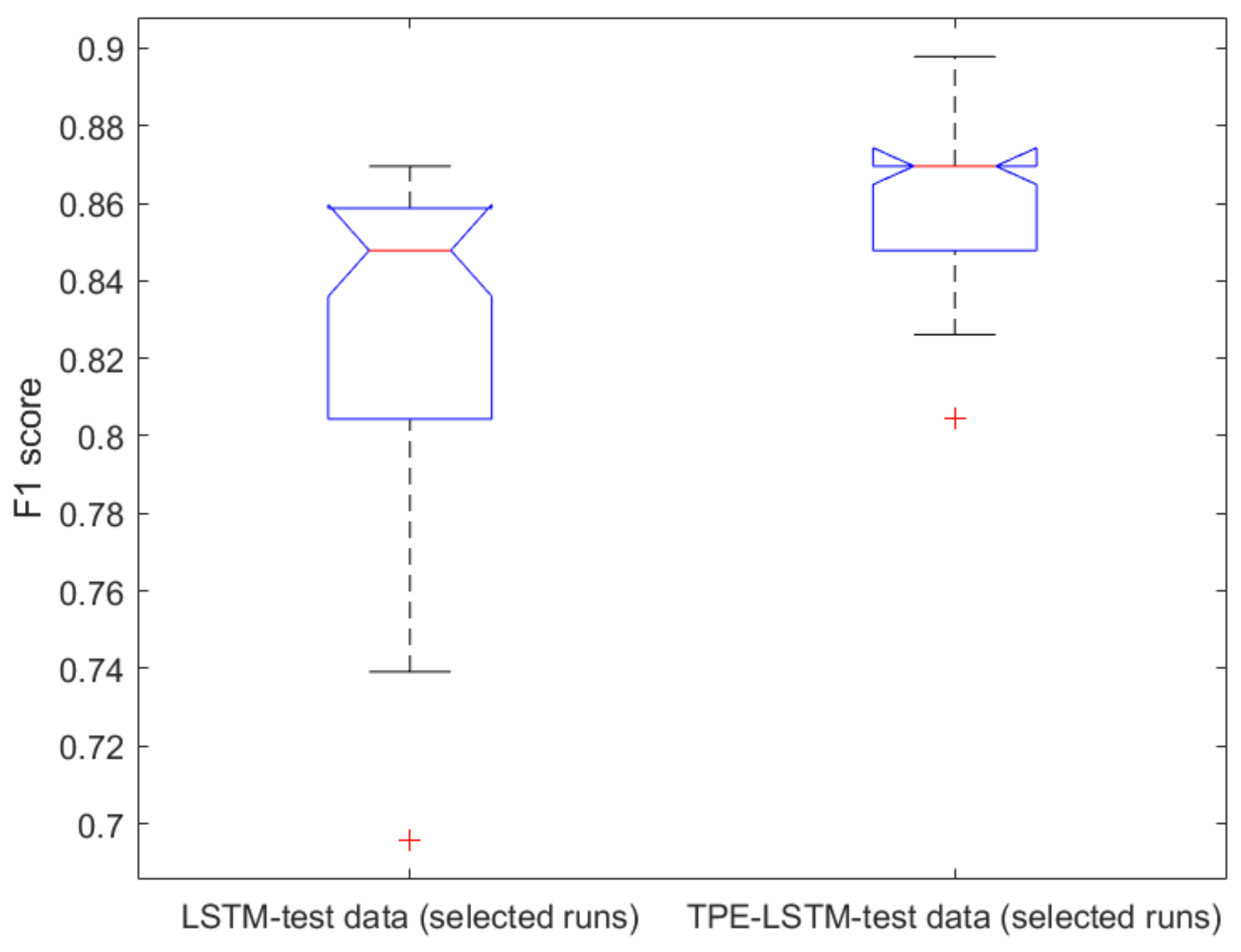
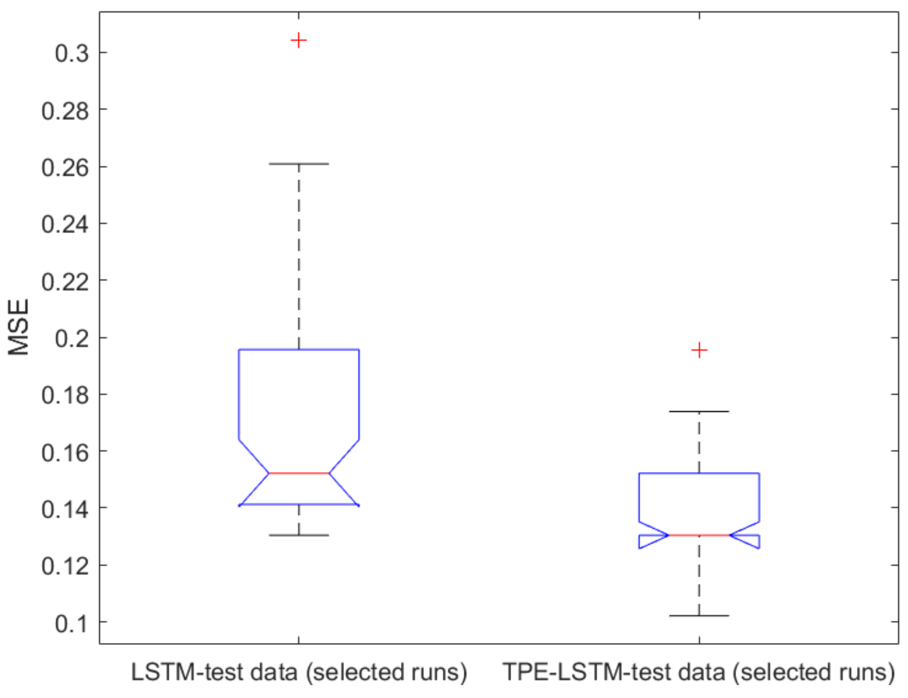
The results displayed below were obtained for Threshold = 0.84. With these parameters, in 52% of runs, TPE improvement was applied.

The mean values and the standard deviation of the MSE indicator and the F1 score when test data are classified are presented in

Table 3. The classification performance: the overall results. Cleveland dataset.

Method	MSE (Mean/Standard Deviation)	F1 Score (Mean/Standard Deviation)
CNN	0.179/0.046	0.821/0.046
LSTM	0.154/0.038	0.846/0.038
TPE-LSTM	0.136/0.019	0.864/0.019

.

Table 4. The classification performance: LSTM selected for improvement versus TPE-LSTM. Cleveland dataset.

Method	MSE (Mean/Standard Deviation)	F1 Score (Mean/Standard Deviation)
LSTM	0.172/0.044	0.827/0.044
TPE-LSTM	0.136/0.020	0.864/0.020

presents the results of classifying test data only for the 52 runs where TPE improvement was applied.

The ANOVA test results are provided in

Table 5. ANOVA table.

Sources	SS	df	MS	F	Prob > F
Groups	0.09245	2	0.04622	34.37	3.73607 × 10−14
Error	0.3994	297	0.00134
Total	0.49185	299

,

Table 6. ANOVA table.

Sources	SS	df	MS	F	Prob > F
Groups	0.09245	2	0.04622	34.37	3.73607 × 10−14
Error	0.3994	297	0.00134
Total	0.49185	299

,

Table 7. ANOVA table.

Sources	SS	df	MS	F	Prob > F
Groups	0.03119	1	0.03119	25.64	1.83117 × 10−6
Error	0.12405	102	0.00122
Total	0.15523	103

and

Table 8. ANOVA table.

Sources	SS	df	MS	F	Prob > F
Groups	0.03119	1	0.03119	25.64	1.83117 × 10−6
Error	0.12405	102	0.00122
Total	0.15523	103

and Figure 1, Figure 2, Figure 3 and Figure 4. Figure 1 shows the results of the ANOVA test applied to compare the F1 scores computed for CNN, LSTM, and TPE-LSTM, while Figure 2 presents the analysis of the MSE values. Figure 3 and Figure 4 present the results of the analysis of the F1 score and MSE indicator for LSTM and TPE-LSTM restricted to the 52% of cases when TPE improvement was applied.

Note that in [5], the best accuracy achieved without feature selection and elimination of outliers was 84.05%, produced by SVM. In our proposal, 2MES-SVM reached 89.2% and TPE-LSTM reached 86.4%. We chose not to use feature selection mechanism because the correlations between the attributes and the target variable could be changed by adding new samples. For instance, this happens when adding Statlog data to the Cleveland Clinical Foundation data and when new examples must be classified.

5.2.2. The Aggregate Dataset

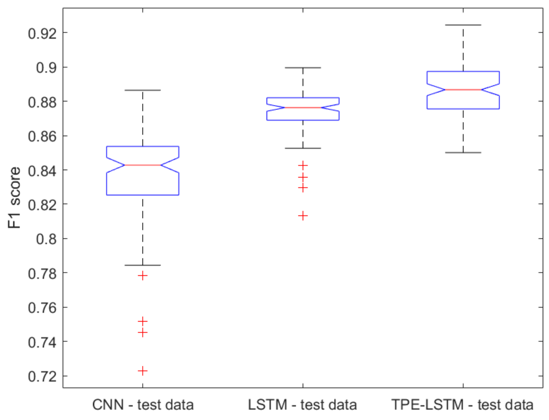
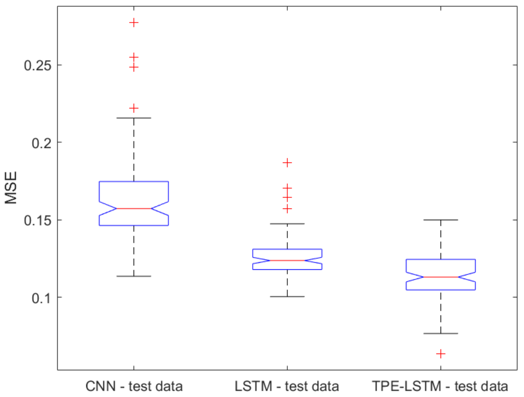
The results displayed below were obtained for Threshold = 0.9. With these parameters, in 86% of runs, TPE improvement was applied.

The mean values and the standard deviation of the MSE indicator and the F1 score when test data are classified are presented in

Table 9. The classification performance: the overall results. Aggregated Cleveland + Statlog dataset.

Method	MSE (Mean/Standard Deviation)	F1 Score (Mean/Standard Deviation)
CNN	0.164/0.030	0.836/0.030
LSTM	0.125/0.014	0.874/0.014
TPE-LSTM	0.113/0.016	0.888/0.016

.

Table 10. The classification performance: LSTM selected for improvement versus TPE-LSTM. Aggregated Cleveland + Statlog dataset.

Method	MSE (Mean/Standard Deviation)	F1 Score (Mean/Standard Deviation)
LSTM	0.126/0.015	0.873/0.015
TPE-LSTM	0.111/0.016	0.889/0.016

presents the results of classifying test data only for the 86 runs where TPE improvement was applied.

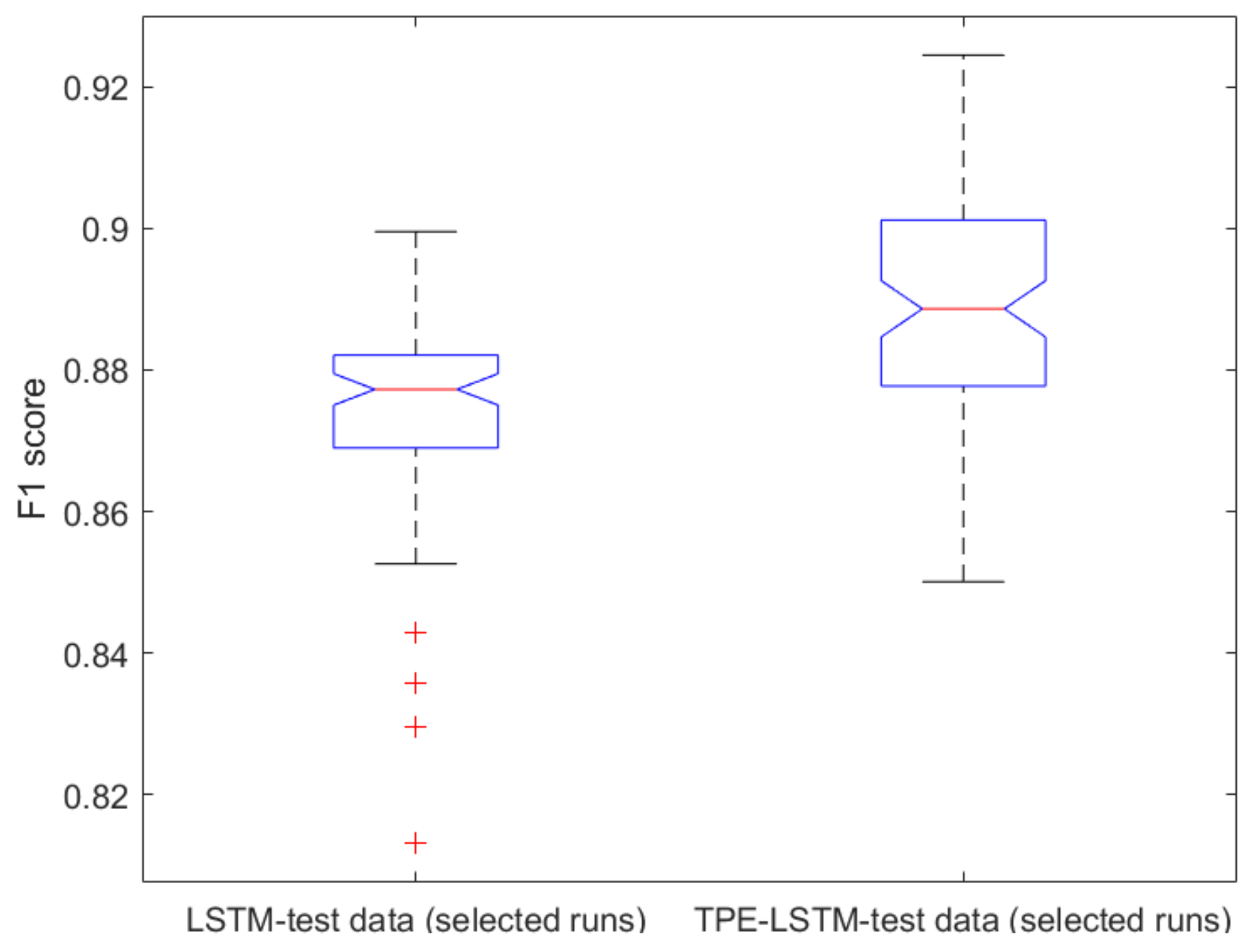
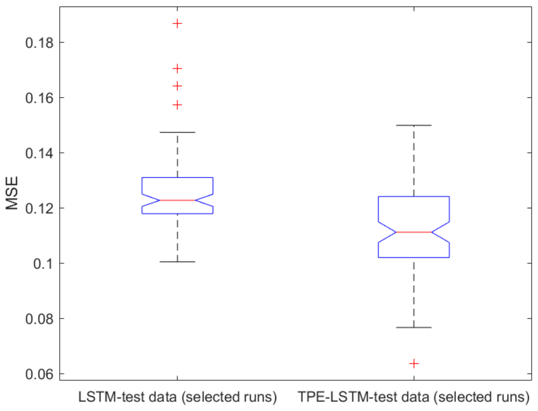
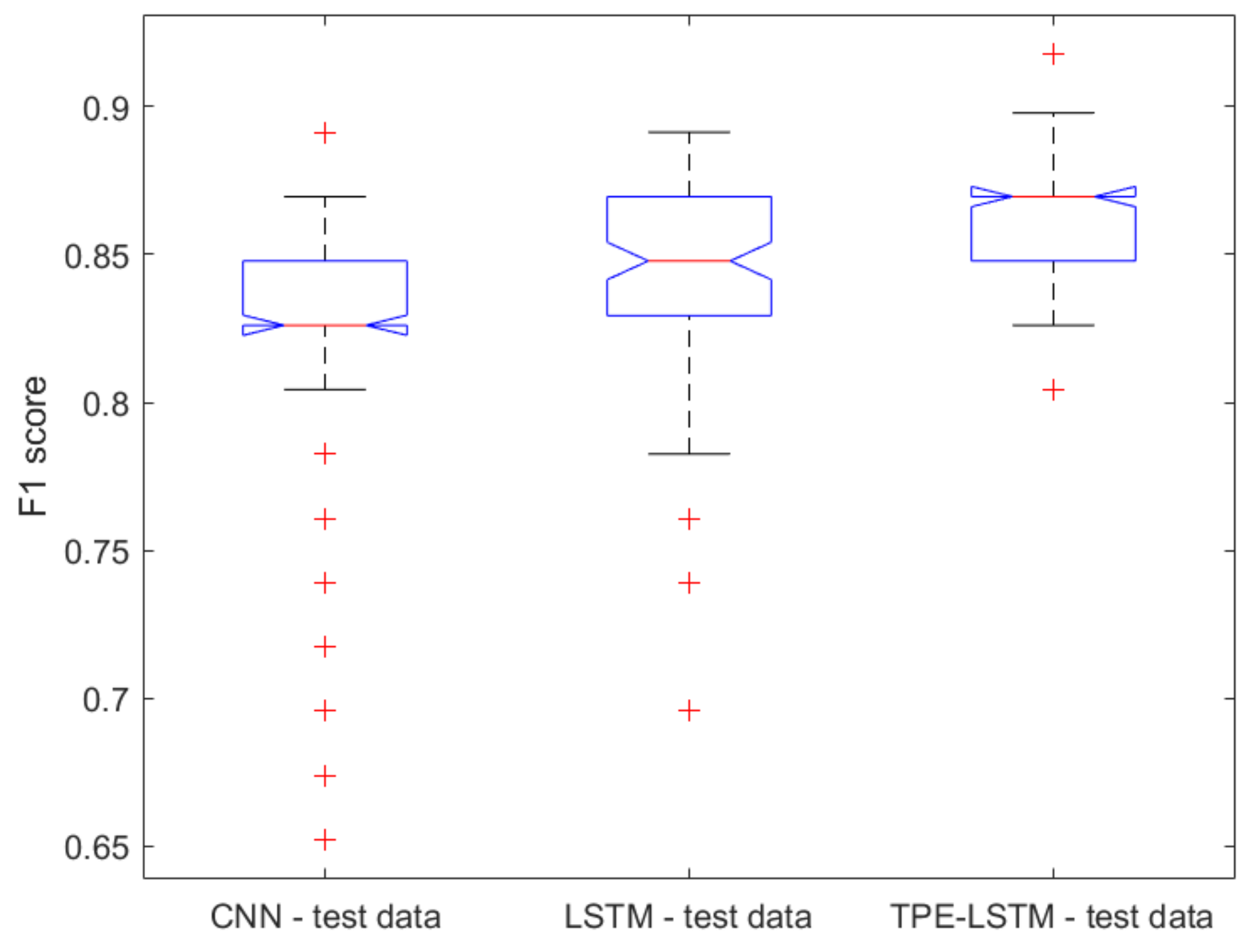
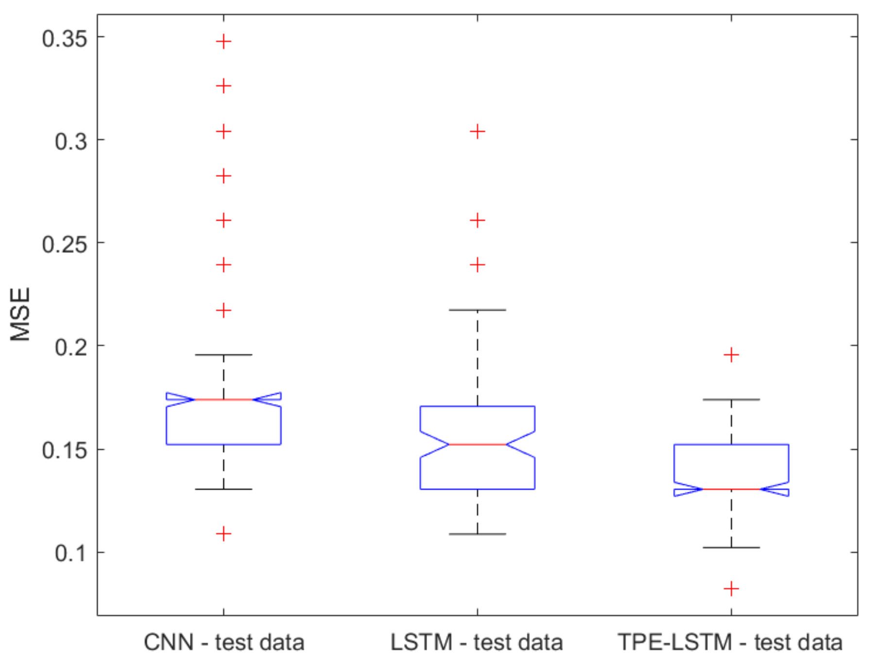
In the following, we provide the ANOVA test results.

Table 11. ANOVA table.

Sources	SS	df	MS	F	Prob > F
Groups	0.14418	2	0.07209	158.28	1.60978 × 10−47
Error	0.13527	297	0.00046
Total	0.27946	299

and Figure 5 show the results of the ANOVA test applied to compare the F1 scores computed for CNN, LSTM, and TPE-LSTM, while

Table 12. ANOVA table.

Sources	SS	df	MS	F	Prob > F
Groups	0.14079	2	0.07039	155.6	5.92892 × 10−47
Error	0.13436	297	0.00045
Total	0.27515	299

and Figure 6 present the analysis of the MSE values.

Table 13. ANOVA table.

Sources	SS	df	MS	F	Prob > F
Groups	0.092	1	0.0092	38.67	3.76083 × 10−9
Error	0.04046	170	0.00024
Total	0.04966	171

and

Table 14. ANOVA table.

Sources	SS	df	MS	F	Prob > F
Groups	0.00869	1	0.00869	35.93	1.9265 × 10−8
Error	0.4114	170	0.00024
Total	0.4983	171

and Figure 7 and Figure 8 present the results of the analysis of the F1 score and MSE indicator for LSTM and TPE-LSTM restricted to the 86% of cases when TPE improvement was applied.

6. Concluding Remarks

This paper investigated the most promising approaches in binary classification for automatic CVD diagnosis and introduced two methods that improve the accuracy of standard classifiers through hyperparameter optimization algorithms. The proposed hybrid approaches are based on the LSTM and SVM models, due to their promising classification performance and generalization capacity. The first algorithm uses the soft-margin non-linear SVM model and 2MES to tune the hyperparameters $\gamma$ and C. The second approach aims to improve the accuracy of a DNN model that is based on a couple of LSTM layers. The classification performance was improved using the TPE algorithm to set the activation functions, the number of hidden neurons, and the dropout rate.

To establish meaningful conclusions, we designed various tests and measured the performance of each classifier using the MSE indicator and the F1 score. The experimentally obtained results pointed out that, as expected, the DNN-based techniques are better suited to solve the problem of CVD diagnosis, based on the Cleveland Clinic Foundation dataset together with its extension Statlog. In the case of the Cleveland Clinic Foundation set, the best results were obtained by the proposed 2MES-SVM, which improves SVM results by 2.5%. In the case of the aggregate dataset, the best results were obtained when using the proposed TPE-LSTM algorithm, with the F1 score being improved by 3.7%. The results are very promising and entail further developments of the DNN-based techniques hybridized with EC algorithms to design automatic diagnosis systems. Additionally, new approaches based on feature extraction preprocessing methods will be considered. We intend to explore the application on unbalanced datasets.

References

1. WHO. CVD Death Estimation. Available online: https://www.who.int/news-room/fact-sheets/detail/cardiovascular-diseases-(cvds) (accessed on 1 September 2022).
2. Cleveland Clinic Foundation. CVD Database. Available online: https://www.kaggle.com/datasets/alexisbcook/cleveland-clinic-foundation-heart-disease (accessed on 1 September 2022).
3. Available online: http://archive.ics.uci.edu/ml/datasets/heart+disease (accessed on 1 September 2022).
4. Available online: https://archive.ics.uci.edu/ml/datasets/statlog+(heart) (accessed on 17 March 2023).
5. Bharti, R.; Khamparia, A.; Shabaz, M.; Dhiman, G.; Pande, S.; Singh, P. Prediction of Heart Disease Using a Combination of Machine Learning and Deep Learning. Comput. Intell. Neurosci. 2021, 2021, 8387680. [Google Scholar] [CrossRef] [PubMed]
6. Karthick, K.; Aruna, S.K.; Samikannu, R.; Kuppusamy, R.; Teekaraman, Y.; Thelkar, A.R. Implementation of a Heart Disease Risk Prediction Model Using. Comput. Math. Methods Med. 2022, 2022, 6517716. [Google Scholar] [CrossRef] [PubMed]
7. Gonsalves, A.H.; Fadi, T.; Rami Mustafa, M.A.; Singh, G. Prediction of Coronary Heart Disease using Machine Learning: An Experimental Analysis. In Proceedings of the 2019 3rd International Conference, Xiamen, China, 5–7 July 2019; pp. 51–56. [Google Scholar]
8. Qi, Z.; Zhang, Z. A hybrid cost-sensitive ensemble for heart disease prediction. BMC Med. Inform. Decis. Mak. 2021, 21, 73. [Google Scholar]
9. Chen, S.-D.; You, J.; Yang, X.-M.; Gu, H.-Q.; Huang, X.-Y.; Liu, H.; Feng, J.-F.; Jiang, Y.; Wang, Y.-J. Machine learning is an effective method to predict the 90-day prognosis of patients with transient ischemic attack and minor stroke. BMC Med. Res. Methodol. 2022, 22, 195. [Google Scholar] [CrossRef]
10. Mohsen, H.; El-Dahshan, E.S.A.; El-Horbaty, E.S.M.; Salem, A.B.M. Classification using deep learning neural networks for brain tumors. Future Comput. Inform. J. 2018, 3, 68–71. [Google Scholar] [CrossRef]
11. Barhoom, A.M.; Almasri, A.; Abu-Nasser, B.S.; Abu-Naser, S.S. Prediction of Heart Disease Using a Collection of Machine and Deep Learning Algorithms. Int. J. Eng. Inf. Syst. (IJEAIS) 2022, 6, 13. [Google Scholar]
12. Dutta, A.; Tamal, B.; Meheli, B.; Acton, S.T. An Efficient Convolutional Neural Network for Coronary Heart Disease Prediction. Expert Syst. Appl. 2020, 159, 113408. [Google Scholar] [CrossRef]
13. Mohan, S.; Thirumalai, C.; Srivastava, G. Effective heart disease prediction using hybrid machine learning techniques. IEEE Access 2019, 7, 81542–81554. [Google Scholar] [CrossRef]
14. El Massari, H.; Gherabi, N.; Mhammedi, S.; Sabouri, Z.; Ghandi, H. ONTOLOGY-BASED DECISION TREE MODEL FOR PREDICTION OF CARDIOVASCULAR DISEASE. Indian J. Comput. Sci. Eng. 2022, 13, 851–859. [Google Scholar] [CrossRef]
15. Aleem, A.; Prateek, G.; Kumar, N. Improving Heart Disease Prediction Using Feature Selection Through Genetic Algorithm. Commun. Comput. Inf. Sci. 2022, 1534, 765–776. [Google Scholar]
16. Durairaj, M.; Revathi, V. Prediction Of Heart Disease Using Back Propagation MLP Algorithm. Int. J. Sci. Technol. Res. 2015, 4, 235–239. [Google Scholar]
17. Al Bataineh, A.; Manacek, S. MLP-PSO Hybrid Algorithm for Heart Disease Prediction. J. Pers. Med. 2022, 12, 1208. [Google Scholar] [CrossRef]
18. Srivastava, K.; Choubey, D.K. Soft Computing, Data Mining, and Machine Learning Approaches in Detection. In Advances in Intelligent Systems and Computing, Proceedings of the 19th International Conference on Hybrid Intelligent Systems, Bhopal, India, 10–12 December 2019; Springer: Cham, Switzerland, 2019; pp. 165–175. [Google Scholar]
19. Suhail, M.M.; Razak, T.A. Cardiac disease detection from ECG signal using discrete wavelet transform with machine learning method. Diabetes Res. Clin. Pract. 2022, 187, 109852. [Google Scholar] [CrossRef]
20. Casalino, G.; Castellano, G.; Kaymak, U.; Zaza, G. Balancing Accuracy and Interpretability through Neuro-Fuzzy Models for Cardiovascular Risk Assessment. In Proceedings of the 2021 IEEE Symposium Series on Computational Intelligence (SSCI), Orlando, FL, USA, 5–7 December 2021; pp. 1–8. [Google Scholar] [CrossRef]
21. Ahmad, Z.; Li, J.; Mahmood, T. Adaptive Hyperparameter Fine-Tuning for Boosting the Robustness and Quality of the Particle Swarm Optimization Algorithm for Non-Linear RBF Neural Network Modelling and Its Applications. Mathematics 2023, 11, 242. [Google Scholar] [CrossRef]
22. Ogundokun, R.O.; Misra, S.; Douglas, M.; Damaševičius, R.; Maskeliūnas, R. Medical Internet-of-Things Based Breast Cancer Diagnosis Using Hyperparameter-Optimized Neural Networks. Future Internet 2022, 14, 153. [Google Scholar] [CrossRef]
23. Prakash, V.J.; Karthikeyan, N.K. Dual-Layer Deep Ensemble Techniques for Classifying Heart Disease. Inf. Technol. Control. 2022, 51, 158–179. [Google Scholar] [CrossRef]
24. Połap, D.; Woźniak, M.; Hołubowski, W.; Damaševičius, R. A heuristic approach to the hyperparameters in training spiking neural networks using spike-timing-dependent plasticity. Neural Comput. Appl. 2022, 34, 13187–13200. [Google Scholar] [CrossRef]
25. Abe, S. Support vector machines for pattern classification. In Advances in Pattern Recognition; Springer: Dordrecht, The Netherlands, 2010; p. 473. [Google Scholar]
26. Alpaydin, E. Introduction to Machine Learning, 2nd ed.; The MIT Press: Cambridge, MA, USA, 2010. [Google Scholar]
27. Menard, S. Applied Logistic Regression Analysis; Sage Publications: Newcastle upon Tyne, UK, 2001; ISBN 0-7619-2208-3. [Google Scholar]
28. Keerthi, S.S.; Duan, K.B.; Shevade, S.K.; Poo, A.N. A Fast Dual Algorithm for Kernel Logistic Regression. Mach. Learn. 2005, 61, 151–165. [Google Scholar] [CrossRef] [Green Version]
29. Joshi, R.; Dhakal, C. Predicting Type 2 Diabetes Using Logistic Regression and Machine Learning Approaches. Int. J. Environ. Res. Public Health 2021, 18, 7346. [Google Scholar] [CrossRef] [PubMed]
30. Chomboon, K.; Chujai, P.; Teerarassamee, P.; Kerdprasop, K.; Kerdprasop, N. An empirical study of distance metrics for k-nearest neighbor algorithm. In Proceedings of the 3rd International Conference on Industrial Application Engineering, Kitakyushu, Japan, 28–31 March 2015. [Google Scholar]
31. Breiman, L. Random Forests. Mach. Learn. 2001, 45, 5–32. [Google Scholar] [CrossRef] [Green Version]
32. Vapnik, V. Statistical Learning Theory; John Wiley: New York, NY, USA, 1998. [Google Scholar]
33. Liu, W.; Príncipe, J.C.; Haykin, S. Kernel Adaptive Filtering: A Comprehensive Introduction; Wiley: Hoboken, NJ, USA, 2011. [Google Scholar]
34. Cocianu, C.; State, L. Kernel-Based Methods for Learning Non-Linear SVM. In Econ. Comput. Econ. Cybern. Stud. Res 2013, 47, 41–60. [Google Scholar]
35. Goodfellow, I.; Bengio, Y.; Courville, A. Deep Learning; MIT Press: Cambridge, MA, USA, 2016; ISBN 978-0-262-03561-3. [Google Scholar]
36. Sheela, K.G.; Deepa, S.N. Review on Methods to Fix Number of Hidden Neurons in Neural Networks. Math. Probl. Eng. 2013, 2013, 425740. [Google Scholar] [CrossRef] [Green Version]
37. Yang, L.; Shami, A. On hyperparameter optimization of machine learning algorithms: Theory and practice. Neurocomputing 2020, 415, 295–316. [Google Scholar] [CrossRef]
38. Siouda, R.; Nemissi, M.; Seridi, H. Diverse activation functions based-hybrid RBF-ELM neural network for medical classification. Evol. Intell. 2022. [Google Scholar] [CrossRef]
39. Bergstra, J.; Bardenet, R.; Bengio, Y.; Kégl, B. Algorithms for Hyper-Parameter Optimization. In Proceedings of the 24th International Conference on Neural Information Processing Systems, Granada, Spain, 12–15 December 2011; pp. 2546–2555. [Google Scholar]
40. Eiben, A.; Smith, J. Introduction to Evolutionary Computing; Springer: Berlin, Germany, 2015. [Google Scholar] [CrossRef]
41. Rong, G.; Li, K.; Su, Y.; Tong, Z.; Liu, X.; Zhang, J.; Zhang, Y.; Li, T. Comparison of Tree-Structured Parzen Estimator Optimization in Three Typical Neural Network Models for Landslide Susceptibility Assessment. Remote Sens. 2021, 13, 4694. [Google Scholar] [CrossRef]
42. Bansal, A.; Singhrova, A. Performance Analysis of Supervised Machine Learning Algorithms for Diabetes and Breast Cancer Dataset. In Proceedings of the 2021 International Conference on Artificial Intelligence and Smart Systems (ICAIS), Coimbatore, India, 25–27 March 2021; pp. 137–143. [Google Scholar] [CrossRef]
43. Wang, L.; Han, M.; Li, X.; Zhang, N.; Cheng, H. Review of Classification Methods on Unbalanced Data Sets. IEEE Access 2021, 9, 64606–64628. [Google Scholar] [CrossRef]
Figure 1. F1 score: test data, all runs. CNN, LSTM, and TPE-LSTM.
Electronics 12 01663 g001
Figure 2. MSE: test data, all runs. CNN, LSTM, and TPE-LSTM.
Electronics 12 01663 g002
Figure 3. F1 score: test data, 52% runs with improvement applied. LSTM versus TPE-LSTM.
Electronics 12 01663 g003
Figure 4. MSE: test data, 52% runs with improvement applied. LSTM versus TPE-LSTM.
Electronics 12 01663 g004
Figure 5. F1 score: test data, all runs. CNN, LSTM, and TPE-LSTM.
Electronics 12 01663 g005
Figure 6. MSE: test data, all runs. CNN, LSTM, and TPE-LSTM.
Electronics 12 01663 g006
Figure 7. F1 score: test data, 86% runs with improvement applied. LSTM versus TPE-LSTM.
Electronics 12 01663 g007
Figure 8. MSE: test data, 86% runs with improvement applied. LSTM versus TPE-LSTM.
Electronics 12 01663 g008