Short Text Sentiment Classification Using Bayesian and Deep Neural Networks

Abstract

The previous multi-layer learning network is easy to fall into local extreme points in supervised learning. If the training samples sufficiently cover future samples, the learned multi-layer weights can be well used to predict new test samples. This paper mainly studies the research and analysis of machine short text sentiment classification based on Bayesian network and deep neural network algorithm. It first introduces Bayesian network and deep neural network algorithms, and analyzes the comments of various social software such as Twitter, Weibo, and other popular emotional communication platforms. Using modeling technology popular reviews are designed to conduct classification research on unigrams, bigrams, parts of speech, dependency labels, and triplet dependencies. The results show that the range of its classification accuracy is the smallest as 0.8116 and the largest as 0.87. These values are obtained when the input nodes of the triple dependency feature are 12,000, and the reconstruction error range of the Boltzmann machine is limited between 7.3175 and 26.5429, and the average classification accuracy is 0.8301. The advantages of triplet dependency features for text representation in text sentiment classification tasks are illustrated. It shows that Bayesian and deep neural network show good advantages in short text emotion classification.

1. Introduction

Sentiment analysis has a long research history in the field of natural language processing. In the past, basically most of the methods were partially based on domain knowledge. Since then, the method based on machine learning has become the mainstream method of sentiment analysis.

In emotion analysis, emotion classification is the most important item. It is based on the emotional information displayed in the text, and divides the text into two or more different categories, that is, a division of the attitudes, views, and tendencies of the text authors. Emotional classification is a new research direction, which has a very important application value in view mining, information prediction, comment classification, garbage filtering, part of speech tagging, public opinion monitoring, etc.

On blog and Weibo data, support vector machine and multinomial naive Bayesian model are tested respectively. It was found that on long texts (blogs), SVMs perform better, while on short texts (microblogs and Twitter), multinomial naive Bayes models outperform.

Based on the analysis of sentiment data flow based on association rules, this paper studies the major events in 2010, and finds that new training data are continuously obtained in the data flow, and studies how to automatically analyze users’ opinions and emotions in a real-time environment.

This paper mainly introduces the deep neural network algorithm, Bayesian regularization deep belief network, machine learning text sentiment classification, tests the role of the meta-learning method based on deep belief network in text sentiment classification, and makes experimental research and analysis, and concludes the desired conclusion. The innovation of this paper is to use the deep neural network algorithm to establish the BR-DBN model and test its performance. The results showed that the model is suitable for discriminative classification problems, and then the experimental research and analysis are carried out in the experimental part, which are closely linked.

2. Related Work

Text sentiment analysis plays an important role in social network information mining. It is also the theoretical basis and basis for personalized recommendation, interest circle classification, and public opinion analysis. Therefore, Chang G proposed a fine-grained short text sentiment analysis method based on machine learning. In order to improve the calculation method of feature selection and weighting, he proposed a sentiment analysis algorithm N-CHI and weight calculation W-TF-IDF which is more suitable for feature extraction, and improved the proportion and weight of sentiment words in feature words through experiments [1]. In addition to the traditional document classification feature set, it is also possible to extract the comments of certain posts as part of the microblog features based on the relationship between the commenter and the poster by constructing a microblog social network as input information. Sun X proposed a Deep Belief Network (DBN) model and a multimodal feature extraction method to extend the features and dimensions of short texts for Chinese microblog sentiment classification [2]. Emotions can be expressed in many ways, such as facial expressions and gestures, speech, and written text. Sentiment analysis in text documents is essentially a content-based classification problem involving concepts from the fields of natural language processing and machine learning. Joshi S discussed techniques used in sentiment recognition and sentiment analysis based on textual data [3]. In recent years, sentiment analysis research has gained a huge impetus on English text data, however, few studies have focused on Nepali text data, and this work focuses on Nepalese text data. Piryani R explored machine learning methods and proposes a dictionary-based approach to sentiment analysis of tweets written in Nepali using linguistic features and lexical resources [4]. Text classification is a central task in natural language processing, aiming to classify text documents into predefined classes or categories. It needs appropriate functions to describe the content and meaning of text documents and map them to target categories. The existing text feature representation depends on the weighted representation of document terms. Therefore, it is very important to choose an appropriate term weighting method, which will help to improve the effectiveness of classification tasks. Attieh J provides a new text classification framework for category-based feature engineering [5]. Naive Bayesian learning algorithm is widely used in many fields, especially in text classification. However, when it is used in fields that violate its naive assumptions, or when the training set is too small to find an accurate probability estimate, its performance will decline. El Hindi K M proposed a naive Bayesian method of inertia fine tuning to solve these two problems [6]. In recent years, the deep learning model has been successfully applied to text emotion analysis. However, category imbalance and unmarked corpus still limit the accuracy of text emotion classification. To overcome these two problems, Jiang W proposed a new text sentiment analysis classification model [7].

Sentiment analysis of online content related to electronic news, products, services, etc., has become very important in this digital age to improve the quality of the services provided. Machine learning-based, knowledge-based, and hybrid are three approaches for sentiment analysis of text, audio, and sentiment. The system proposed by Divate MS is a polarity-based sentiment analysis of Marathi electronic news [8]. Twitter is an online blogging site on the Internet that provides a platform for people to experience and talk about their thoughts on troubles, events, merchandise, and exclusive ideas. Bhagat C proposed that its most important goal is to have a comprehensive understanding of the way machine learning strategies are used in sentiment analysis in order to get better results in short details [9]. Sentiment analysis is one of the main fields of natural language processing, and its main task is to extract sentiments, opinions, attitudes, and emotions from subjective texts. Due to its importance in decision-making and people’s trust in website reviews, there are many academic studies addressing the SA problem. So, Albayati A Q proposed deep learning to explore powerful machine learning techniques, emerging with its feature representation and ability to discriminate data, resulting in state-of-the-art prediction results [10]. Social network data are unstructured and unpredictable, and contain idioms, jargon, and dynamic themes. Machine learning algorithms for traffic event detection may not be able to extract valuable information from social network data. Farman Ali proposed a real-time monitoring framework based on social networks for traffic accident detection and condition analysis using ontology and potential Dirichlet assignment as well as two-way short-term and short-term memory [11]. In the emotional attitude extraction task, the goal is to identify the “attitude”—emotional relationship between the entities mentioned in the text. Rusnachenko N studied attention-based context coder in emotional attitude extraction task [12]. The views put forward by these scholars are all in line with the current situation of emotional texts, and this research has great research significance. However, they all overlooked a very important point, that is, they did not clarify their research objects. Therefore, this paper will focus on an investigation and analysis combining algorithm experiments and actual research objects.

3. Bayesian Network and Deep Neural Network Algorithm

3.1. Deep Neural Network Algorithm

Deep learning is a research field of machine learning. It studies the distribution rules of data, so that the machine can have the same learning ability as humans, and have certain recognition ability for images and sounds. In recent years, with the great success of deep learning in computer vision, speech recognition, data mining, and many other fields, it also has difficulties that traditional methods cannot overcome. Therefore, it has become a new research hotspot. Deep learning uses more complex neural networks to solve problems. Face recognition technology is ubiquitous in daily life, and face recognition is a relatively important in-depth learning direction. For neural network, face is like a data matrix. The top layer is used to extract facial features, and the bottom layer is used to recognize facial features.

(1) Deep self-encoding network

Encoder is a device that encodes a signal or data into a signal that can be communicated, transmitted, and stored. The encoder converts angular displacement and linear displacement into electrical signals. According to the different reading modes, the encoder can be divided into contact type and non-contact type. According to the working principle of coding, the coding device can be divided into incremental coding device and absolute value coding device. Encoder appeared in the 1980s, which is a control-free learning algorithm. The basic idea of Encoder is to match the input network as much as possible. The encoding process consists of the input layer to form the hidden layer, and the decoding process consists of the hidden layer to the output layer. Figure 1 shows the overall framework of this paper.

(2) Deep belief network

In the deep belief network, the energy function refers to the function used to calculate the “energy” or “cost” of each state in the network. Energy function is one of the core concepts in deep belief network, which can describe the complexity of the model and the adaptability of the model to data. During the training process, the network parameters are iteratively optimized to minimize the energy function on the training data. When the network parameters are fixed, the energy function can be used to evaluate whether the new data conform to the network distribution. Suppose layer d has m visible units and layer g has n hidden units. Then the energy function between the visible layer node and the hidden layer node $(d,g)$ is:

$$P(d,g|\alpha )=-{\displaystyle \sum _{n=1}^m{x}_j{d}_j-{\displaystyle \sum _{n=1}^m{y}_i{g}_i}}-{\displaystyle \sum _{n=1}^m{\displaystyle \sum _{m=1}^n{d}_j{w}_{ji}{g}_i}}$$

(1)

The joint probability distribution of $(d,g)$ can be obtained as:

$$E(d,g|\alpha )=\frac{p^{-p(d,g|\alpha )}}{z(\alpha )}$$

(2)

In which,

$$\mathrm{z}(\alpha )={\displaystyle {\sum }_{d,g}{p}^{-p(d,g|\alpha )}}$$

(3)

Then the likelihood functions $E(d|\alpha )$ and $E(g|\alpha )$ can be expressed as:

$$E(d|\alpha )=\frac{1}{z(\alpha )}{\displaystyle \sum _g{p}^{-p(d,g|\alpha )}}$$

(4)

$$E(g|\alpha )=\frac{1}{z(\alpha )}{\displaystyle \sum _d{p}^{-p(d,g|\alpha )}}$$

(5)

In addition, the conditional probabilities $E(d|g;\alpha )$ and $E(g|d;\alpha )$ of the hidden layer and visible layer can also be obtained as:

$$E(d|g;\alpha )=\frac{E(d,g|\alpha )}{E(g|\alpha )}=\frac{\frac{1}{z(\alpha )}{p}^{-p(d,g|\alpha )}}{\frac{1}{z(\alpha )}{\displaystyle \sum _d{p}^{-p(d,g|\alpha )}}}=\frac{p^{-p(d,g|\alpha )}}{{\displaystyle \sum _d{p}^{-p(d,g|\alpha )}}}$$

(6)

$$E(g|d;\alpha )=\frac{E(d,g|\alpha )}{E(d|\alpha )}=\frac{\frac{1}{z(\alpha )}{p}^{-p(d,g|\alpha )}}{\frac{1}{z(\alpha )}{\displaystyle \sum _g{p}^{-p(d,g|\alpha )}}}=\frac{p^{-p(d,g|\alpha )}}{{\displaystyle \sum _g{p}^{-p(d,g|\alpha )}}}$$

(7)

Since there is no connection between the hidden layer and the visible layer, the activation function can be derived from Equations (6) and (7), respectively:

$$E(d_j=1|g;\alpha )=\frac{1}{1+p^{-x_j-{\displaystyle {\sum }_i{w}_{ji}{g}_i}}}$$

(8)

$$E(g_j=1|d;\alpha )=\frac{1}{1+p^{-y_i-{\displaystyle {\sum }_j{w}_{ji}{d}_j}}}$$

(9)

Learning an RBM is about determining what is best for learning the data. This value can be obtained by minimizing the gradient and maximizing the likelihood function. In order to simplify the calculation, the logarithm can be increased, and the key step is to find the partial derivative of 2 in Learning an RBM is about determining what is best for learning the data. This value can be obtained by minimizing the gradient and maximizing the likelihood function. In order to simplify the calculation, the logarithm can be increased, and the key step is to find the partial derivative of $\alpha$ in 1, namely:

$$\frac{\eta InE(d|\alpha )}{\eta \alpha }={\displaystyle \sum \left[{\frac{\eta (p(d,g|\alpha ))}{\eta \alpha }}_{E(g|d,\alpha )}-{\frac{\eta (p(d,g|\alpha ))}{\eta \alpha }}_{E(d|g,\alpha )}\right]}$$

(10)

Since $\alpha =\left\{w_{ji},x_j,y_i\right\}$, the partial derivative of $w_{ji},x_j,y_i$ can be obtained as:

$$\frac{\eta InE(d|\alpha )}{\eta w_{ji}}=d_j{g}_{i_{E(g|d,\alpha )}}-d_j{g}_{i_{E(d,g|\alpha )}}$$

(11)

Currently, in RBM algorithms, fast algorithms are usually used to approximately sample the reconstructed data to update parameter values.

3.2. Bayesian Regularization Deep Belief Networks

The Bayesian Regularization BR (Bayesian Regularization) method is a Bayesian inference method to determine the hyperparameters in the regularization method. At present, it has been applied in the research of image recognition, medicine, economy, and other fields. Bayesian regularization algorithm provides a new idea for improving the generalization ability of neural network, and has been widely recognized in many fields of research. Its network structure diagram is shown in Figure 2.

The purpose of this paper is to apply the Bayesian regularization algorithm to the RBM algorithm to improve the generalization ability of DBN.

Suppose the function is:

$$Q=\frac{1}{2}{\displaystyle \sum _{v=1}^V{\displaystyle \sum _{m=1}^M{(b_{mv}-c_{mv})}^2}}$$

(12)

where V represents the number of output nodes; M represents the number of training sets; $b_{mv}$ represents the expected output value; $c_{mv}$ represents the actual output value. Then, using the regularization method, the training function becomes:

$$P=\beta \cdot Q+\phi Q_W=\beta Q+\phi Q_W$$

(13)

In the formula, P is the new learning function, $\beta$ and $\phi$ are the hyperparameters that determine the distribution of parameters such as weights and thresholds.

Hyperparametric optimization refers to the process of finding the optimal combination of hyperparameters in machine learning to improve the performance and effectiveness of the models. Common hyperparametric optimization methods include grid search, random search, Bayesian optimization, and automatic machine learning. Among them, grid search is a violent search method, which will train all possible combinations of super parameters; random search is a method of randomly selecting super parameters, which can achieve the balance between calculation cost and effect; Bayesian optimization is an optimization method based on Bayesian theorem, which can gradually adjust the value range of superparameters according to the performance of known superparameter combinations to find the optimal superparameter combination; automatic machine learning is an automatic machine learning method, which can automatically select the optimal model and super-parameter combination, and can transfer learning in multiple tasks, thus improving the generalization ability of the model.

3.3. Bayesian Regularized Deep Belief Network Model

(1) Model construction

This paper constructs a BR DBN model whose bottom is superimposed by multilayer Bayesian regularization RBM (BR RBM). The frame is shown in Figure 3. Back-propagation is to calculate the partial derivatives of each layer in the opposite direction according to the loss function, so as to update the parameters.

(2) Model training

The completed state of each layer of BR-RBM is used as the input of the next layer of BR-RBM, and the process is repeated until the pre-training of all BR-RBM layers is completed [13].

Assuming that the BR-DBN network consists of m layers of BR-RBM, since the tuning phase starts from the last layer of BR-DBN, set the output vector of the last layer to be $f^m(a)$, that is, the initial sample is a, then $f^m(a)$ is:

$$f^m(a)=\frac{1}{1+p^{(y^m+w^m{f}^{m-1}(a))}}$$

(14)

In the formula, $y^m$ and $w^m$ are the bias value and weight of the 1st layer BR-RBM respectively; $f^{m-1}$ is the output vector of the m − 1th layer. After the forward l-layer BR-RBM learning, it can be concluded that the jth sample belongs to the category. The probability of $b_j\in (1,2,\dots k)$ is:

$$q(b_j=r|f^m(a_j),D^m,k^m)=\frac{p^{D_r^m{f}^m(a_j)+k^m}}{{\displaystyle {\sum }_{r=1}^k{p}^{D_r^m{f}^m(a_j)+k^m}}}$$

(15)

In the formula, D is used as a parameter coefficient, and the category corresponding to the maximum probability is the category judged by BPNN. The formula for the error function of the mth layer is:

$$S({\epsilon }^m)=-\frac{1}{n}\left[{\displaystyle \sum _{j=1}^1{\displaystyle \sum _{r=1}^{k}1\left\{b_j=r\right\}\log \frac{p^{D_r^m{f}^m(a_j)+k^m}}{{\displaystyle {\sum }_{r=1}^k{p}^{D_r^m{f}^m(a_j)+k^m}}}}}\right]$$

(16)

In the formula, ${\epsilon }^m=\left\{w^m,y^m,k^m,D^m\right\}$ and $1\left\{b_j=r\right\}$ are used as the logical indicator function, when $b_j=r$, the value is equal to 1; when $b_j\ne r$, the value is equal to 0. To find the minimum value of the error, use gradient ascent to find the partial derivatives of the parameters as follows:

$${\nabla }_{{\epsilon }^m}S({\epsilon }^m)=\frac{1}{n}{\displaystyle \sum _{j=1}^n\left[f^m({\stackrel{⌢}{a}}_j)(1\left\{b_j=r\right\}-g^m({\stackrel{⌢}{a}}_j))\right]}$$

(17)

If the number of hyperparameters is very large, use random search to find the potential combination of hyperparameters, and then use the local grid search to select the optimal feature. Next, super-parameter trimming, the formula is:

$${\epsilon }^m={\epsilon }^m-\beta {\nabla }_{\epsilon }-S({\epsilon }^m)$$

(18)

In the formula, $\beta$ represents the learning rate.

(3) Model performance test

The BR-DBN model constructed in this paper is used to discriminate and classify several commonly used standard datasets. Initialize W, x, y, random small values that obey a Gaussian distribution. The initial learning rate is set to 0.1, and the learning rate variation coefficient is set to 0.01, and the test results are shown in

Table 1. Classification test results on different standard datasets.

Data Set	Training Set	Test Set	Average Classification Error Rate %
Iris	100	50	1.97
Seeds	150	60	3.46
Perfume Data	320	150	2.87
Four class	500	200	2.59

[14].

As can be seen from Table 1, for different datasets, the BR-DBN model has a lower average error rate, and the results show that the model is suitable for discriminative classification problems. Error rate refers to the proportion of the number of samples with incorrect classification to the total number of samples.

4. Machine Text Emotion Classification Experiment Based on Deep Belief Network

4.1. Experimental Design

The manual annotation-based supervised learning algorithm in this paper uses a language model. Language models can be probabilistic based or non-probabilistic. Twitter emotion analysis is actually a classification problem. In order to use language models to conduct twitter emotion analysis, this article combines twitter short essays from the same class (positive or negative) to form a large document. The learning process of the affective language model is similar to the subjective classification problem, except that the category becomes both subjective and objective [15].

Recently, in the field of twitter short text sentiment analysis, there are more and more learning algorithms that do not need manually annotated data [16]. Such algorithms learn the classifiers from the training data with noisy annotations, which are emoticons or other specific markers. The advantage of these learning algorithms is that they eliminate the heavy manual annotation process. A large number of training data with noisy annotation information can be automatically obtained through programs, including twitter’s open API or other existing twitter emotion analysis websites. Although a number of noise-annotation-based algorithms have been proposed. However, there are still some flaws in these methods.

First, none of these methods solve the problem of subjective classification very well. Second, they all need to climb a large number of twitter short texts and store them locally, considering that the twitter crawl is limited, so it is also a time-consuming and inefficient way. Third, because the annotation information is inherently noisy, the classifier obtained only using such training data with noisy annotation has limited accuracy. Fourth, at present, few models can effectively use the artificial annotation information and the noise annotation information simultaneously to integrate these two kinds of information into a set of framework.

For subjectivity classification, the two sentiment categories are subjective and objective. This paper assumes that tweets containing “:)” or “:(” are subjectively colored by the publisher. Therefore, the search phrase posted to the twitter search API constructed in this paper is “:)” or “:(”, which is used to estimate the subjective emotion language model [17].

For the language model of objective emotion, it is more difficult to calculate Pu(|), that is, the occurrence probability of words in the objective emotion category, than the subjective category. To the best of our knowledge, no academics have made valid assumptions about objective tweets. This paper has tried a hypothetical strategy such that if a tweet does not contain any expressions, then it is likely to be objective. The experimental results show that this hypothesis is not satisfactory. It tries to use hashtags, such as “#jobs”, as tags for objective tweets, but there are some problems with this assumption. For one, the number of tweets that contain specific hashtags is limited. Second, the sentiment of tweets can bias specific hashtags, such as “#jobs,” without ensuring objectivity.

In this paper, we propose a novel hypothesis to label objective tweets. If a tweet contains an objective url link, it is more likely to be objective. Based on our observations, we find that if url links come from image sites (such as twitpic.com) or video sites (such as youtube.com), they are likely to be subjective. But if the url link is from a news site, there is a good chance it is an objective tweet. Therefore, if a url link does not come from a picture website or a video website, this article calls this url an objective url link. Based on the above findings and assumptions, the search phrase submitted to the twitter search API constructed in this paper is “wifilter:links”, where filter:links indicates that the returned tweets are linked by url. This paper does this to obtain the information of objective tweets [18].

Considering that both algorithms based on manual annotation and only using noise annotation information have their own disadvantages, the best strategy is to use both manual and noise annotation information and use two types of training data for model training. How to seamlessly integrate these two different types of data into a unified framework is the challenge addressed in this chapter. This paper presents a brand new model, based on the emoji smoothing language model, namely emoticonsmoothedlanguagemodel (ESLAM).

The main contributions of ESLAM are as follows:

After training the language model through manually annotated data, ESLAM smoothed the language model using training data annotated with emoticons. Thus, ESLAM seamlessly integrates manual and noisy annotated data to form a unified probabilistic model framework. The large amount of noise annotation data allows the ESLAM language model to handle misspelled words, slang, tone words, abbreviations, and their various unlogged words. This ability is not found in a common supervised learning model based on manual annotation.

In addition to discriminating between positive and negative polarity classification, ESLAM can also be used for subjective classification. The previous noise annotation-based algorithm cannot be used for subjective classification.

Most noise annotation-based learning algorithms need to crawl a large number of twitter short texts and store them locally, but considering that twitter crawling has access frequency limited, it is also a time-consuming, storage space consuming and inefficient way [19]. The ESLAM in this paper proposes an innovative and simple method to directly estimate the probability of each word in the language model by using twitter’s open API, without the need to download any original text from twitter.

Experiments on real data from twitter show that ESLAM can effectively integrate artificial and noise annotation information and work better than other algorithmic models that use only one of these information.

To test the role of meta-learning methods based on deep belief networks in text emotion classification, two sets of contrast experiments were used. The first group compares the results of the meta-learning method of deep belief network and the deep belief network directly acting on the text feature vector in text emotion classification, and the results of metalearning and fixed rules in text emotion classification.

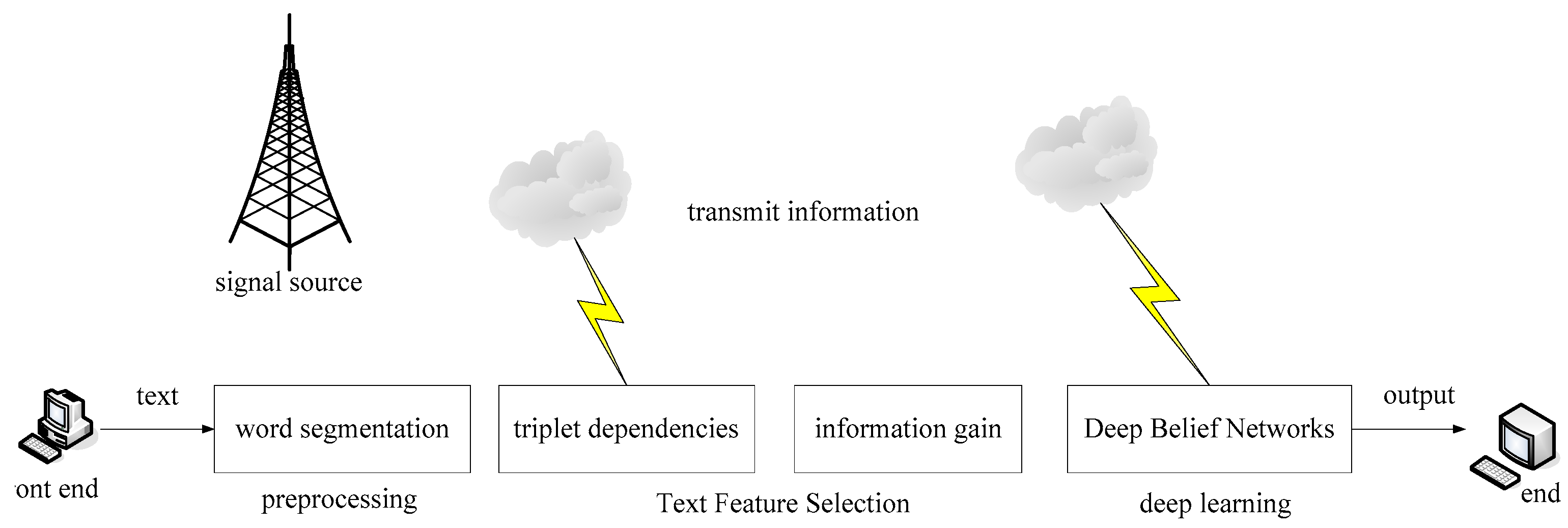
The deep persuasion of the network directly affects the emotional classification of the text. The work process consists of three parts: text pre-processing, text feature selection, and learning in the deep neural network. The process is shown in Figure 4.

Figure 4 shows the process from the original text of using the deep belief network to obtain the classification results. First, the preprocessing steps of sentence sentences, polarity annotation, and word segmentation are carried out. Then, on the basis of word segmentation, the onery words of sentences, binary words, word sex, dependency label, ternary dependency relationship and other characteristics of the sentence are extracted to form the text representation vector. In general, for the feature vector space with large dimension, the information gain feature selection algorithm is used. Finally, the training set is used for the deep belief network for training to obtain the determined network structure. The network structure was tested with the test set, and the final available deep belief network was determined by adjusting the corresponding network structure and parameters [20].

This paper uses a publicly available Sanders dataset containing 5513 manually annotated tweets. The tweets are all about one of the four themes, namely Apple, Google, Microsoft, and Twitter. After removing non-English tweets and junk tweets, there are still 3723 tweets left. The larger the index value, the more accurate the text emotion classification results are. Six sets of different features were selected, including monary word, binary word, word sex, dependency label, combined features of emotion score, and triplet dependency feature. The dimensions of each functional set were network input with 1000, 2000, 4000, 6000, 8000, 12000, 14000 items with the highest information gain score. The number of different network layers and their corresponding hidden layer nodes are shown in

Table 2. Deep belief network structure settings.

Number of Hidden Layers	Network Structure
2	X-600-300
3	X-600-300-100
5	X-2000-300-200-100

.

In Table 2, the network structure with X representing the input nodes and 2 layers is X-600-300, indicating the first hidden layer knots of 600 and the second hidden layer knots of 300.

Experimental results record the classification accuracy and reconstruction error of different feature dimensions under different network structures. It records the accuracy of the network DBN: X-2000-1000-500-200-100, DBN: X-600-300-100, DBN: X-600-300 and BP: X-600 in different dimensions of six sets of feature sets. The reconstruction errors are numbered according to the corresponding number of hidden layers.

4.2. Classification and Calculation

Experimental calculations were performed according to the experimental flow in Figure 5. Experimental results record the classification accuracy and reconstruction error of different feature dimensions under different network structures. They are the results of network DBN: X-2000-1000-500-200-100, DBN: X-600-300-100, DBN: X-600-300, and BP: X-600 in different dimensions of six sets of feature sets. The reconstruction errors are numbered according to the corresponding number of hidden layers [21].

The minimum, maximum, and mean values of the source data results were calculated. Statistical results are presented in

Table 3. DBN: X2000-1000-500-200-100 statistical results.

	Exact Value	Reconstruction Error 1	Reconstruction Error 2	Reconstruction Error 3	Reconstruction Error 4	Reconstruction Error 5	Time (s)
minimum	0.8058	9.4408	0.6078	2.4241	2.4355	1.4961	1696.6
Imaximum value	0.8692	22.5905	10.3566	5.2308	5.2445	4.3040	4970.7
average value	0.8303	16.0944	8.7713	3.9798	4.1796	3.0649	3208.9

,

Table 4. DBN: X600-300-100 statistical results.

	Exact Value	Reconstruction Error 1	Reconstruction Error 2	Reconstruction Error 3	Time (s)
minimum	0.8116	7.3175	2.7168	1.3974	166.3
maximum value	0.8700	26.5429	6.2811	4.4129	1503.6
average value	0.8301	15.9288	4.9615	2.9398	763.4

,

Table 5. DBN: X600-300 statistical results.

	Exact Value	Reconstruction Error 1	Reconstruction Error 2	Time (s)
minimum	0.8000	7.3296	2.7044	142.2
maximum value	0.8700	26.5921	9.5712	1117.5
average value	0.8327	16.1251	5.0907	717.4

and

Table 6. DBN: X600 statistical results.

	Exact Value	Time (s)
minimum	0.8133	45.35
maximum value	0.8641	1117.5
average value	0.8333	322.3

.

Table 3 shows the results of the network DBN: X-2000-1000-500-200-100. Among them, the minimum classification accuracy was 0.8058 and the maximum was 0.8692, obtained when the triplet dependency feature dimension was 14,000, the average classification accuracy of the 5-layer deep belief network was 0.8303. However, the first-layer restricted Boltzmann machine reconstruction error for a single training set is 9.4408 to 22.5903, and the average reconstruction error is 16.0944. The reconstruction error increases with the input nodes. The reconstruction error in the second layer ranged from 6.0798 to 10.3566, with an average value of 8.7713. The first layer is greatly reduced in the reconstruction error. The reconstruction error of the third layer ranges from 2.4241 to 5.2308, and the average reconstruction error is 3.9798, which is also reduced from the reconstruction error of the second layer. The fourth layer reconstruction error ranged from 2.4355 to 5.2445, with an average of 4.1796, and the third layer showed little change. The reconstruction error in the fifth layer ranges from 1.4961 to 4.3040, with an average of 3.0649, decreasing compared with the reconstruction error in the previous layer. The network running time ranged from 166.3 to 1503.6 s, increasing with increasing input nodes.

Table 4 shows the results of the network DBN: X-600-300-100. Among them, the minimum range of classification accuracy is 0.8116, the maximum is 0.87, taken when the triplet dependency feature input node is 12,000, the average classification accuracy is 0.8301. The reconstruction error range of the first layer confined Boltzmann machine is between 7.3175 and 26.5429, increasing with increasing input nodes. The reconstruction error of the second layer ranges from 2.7168 to 6.2811, which is less accurate from that of the previous layer. The reconstruction error of the third layer ranges from 1.3974 to 4.4129, which is also reduced compared with the previous layer. The time period ranged from 166.3 s to 1503.6 s.

Table 5 shows the results of the network DBN: X-600-300. Among them, the minimum classification accuracy was at 0.8116 and the maximum was 0.87, obtained when the triplet dependency feature input node was 14,000, and the average classification accuracy was 0.8326. However, the reconstruction error range of the training set is 7.3296 to 26.5921, increasing with more input nodes. The reconstruction error in the second layer ranges from 2.7044 to 9.5712, which is lower than that of the previous layer. The time period ranged from 142.2 s to 1409.4 s.

Table 6 shows the results of network BP: X-600. Among them, the minimum classification accuracy was 0.8133 and the maximum was 0.8641, obtained when the ternary dependency feature input dimension was 14,000, and the average classification accuracy was 0.8333. The time period ranged from 45.35 s to 1117.5 s.

4.3. Experimental

(1) Effect of different feature sets on the classification accuracy

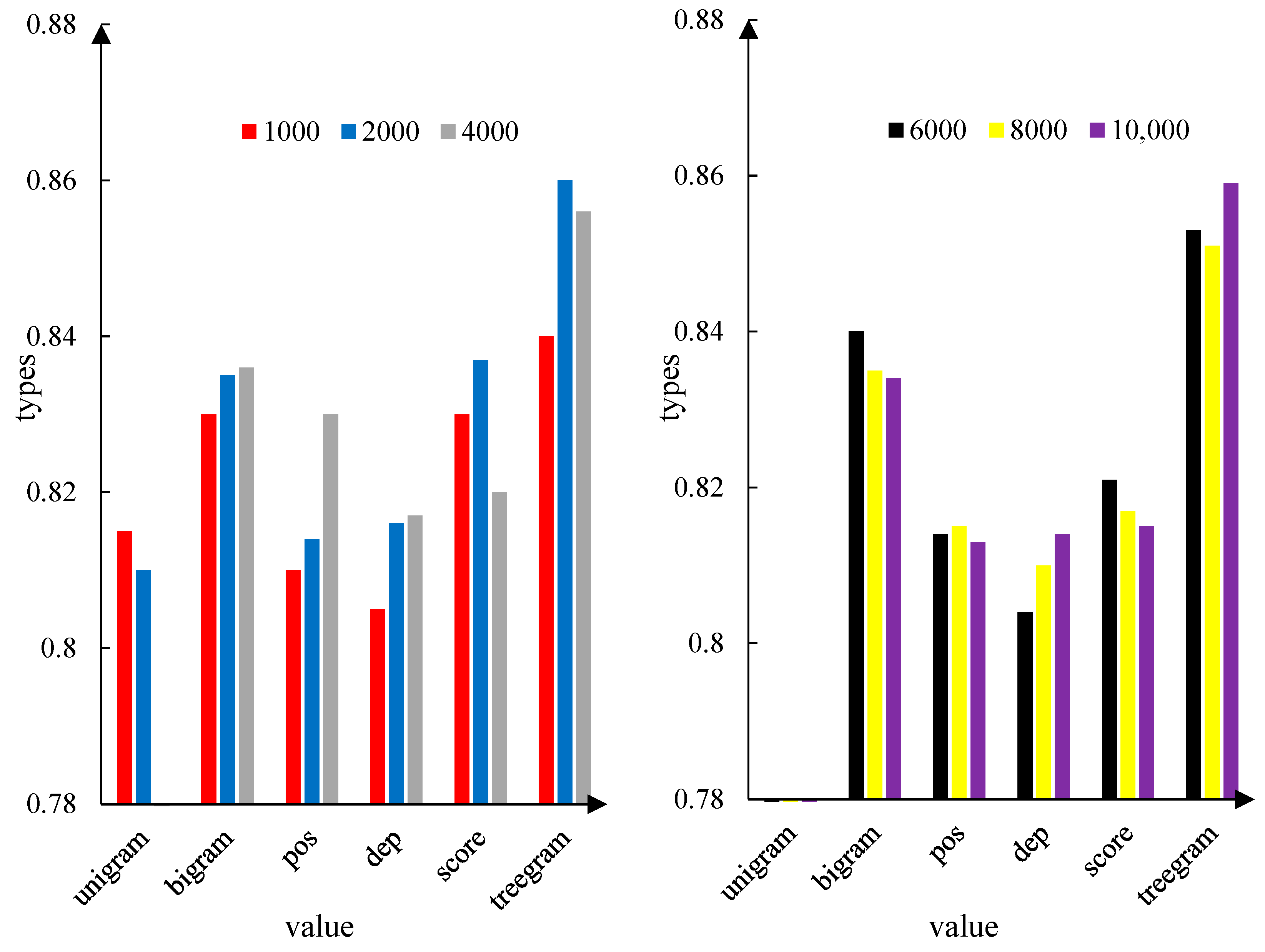
As can also be seen from Figure 5, in order to verify numerical, by calculating the average classification accuracy of different feature sets, the results are 0.81, 0.8381, 0.8195, 0.8152, 0.8220, and 0.8620. The highest classification accuracies were 0.8142, 0.8433, 0.8308, 0.825, 0.8342, and 0.8692, respectively. We show that the triple dependence is a feature representation that achieves the highest classification accuracy, followed by combined features of monary and binary words.

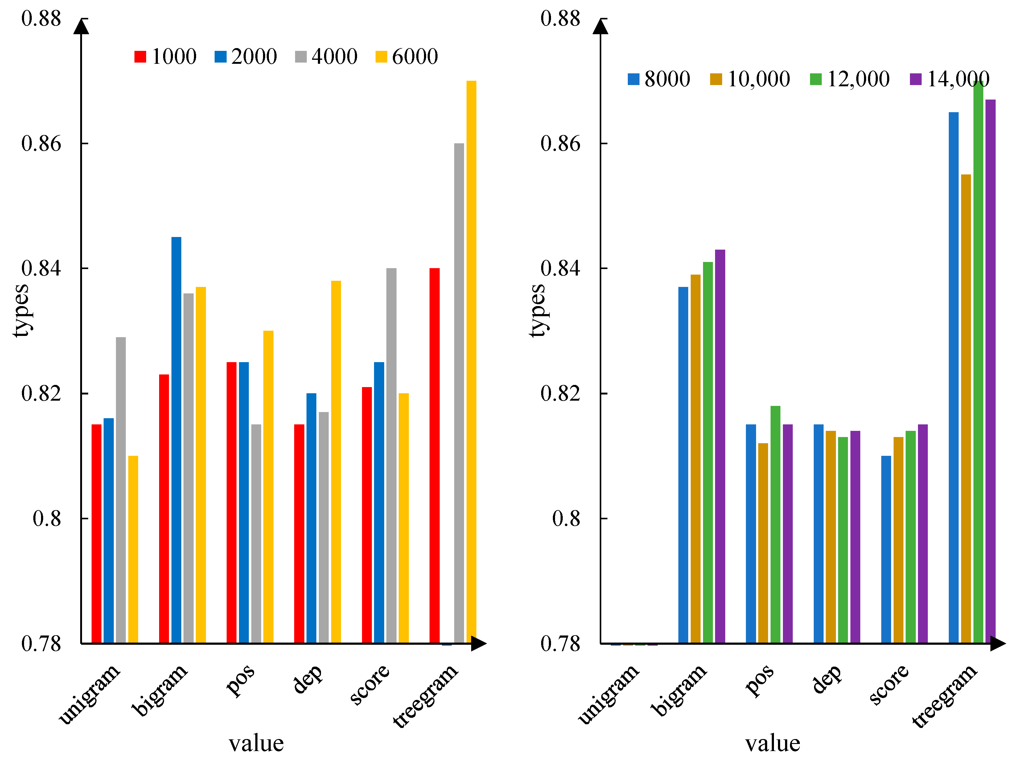
As can be seen from Figure 6, the average classification accuracy according to different feature sets is 0.8202, 0.8379, 0.8214, 0.8175, 0.8215, and 0.8585. The highest classification accuracy obtained was 0.8291, 0.845, 0.8283, 0.8325, 0.8375, and 0.87.

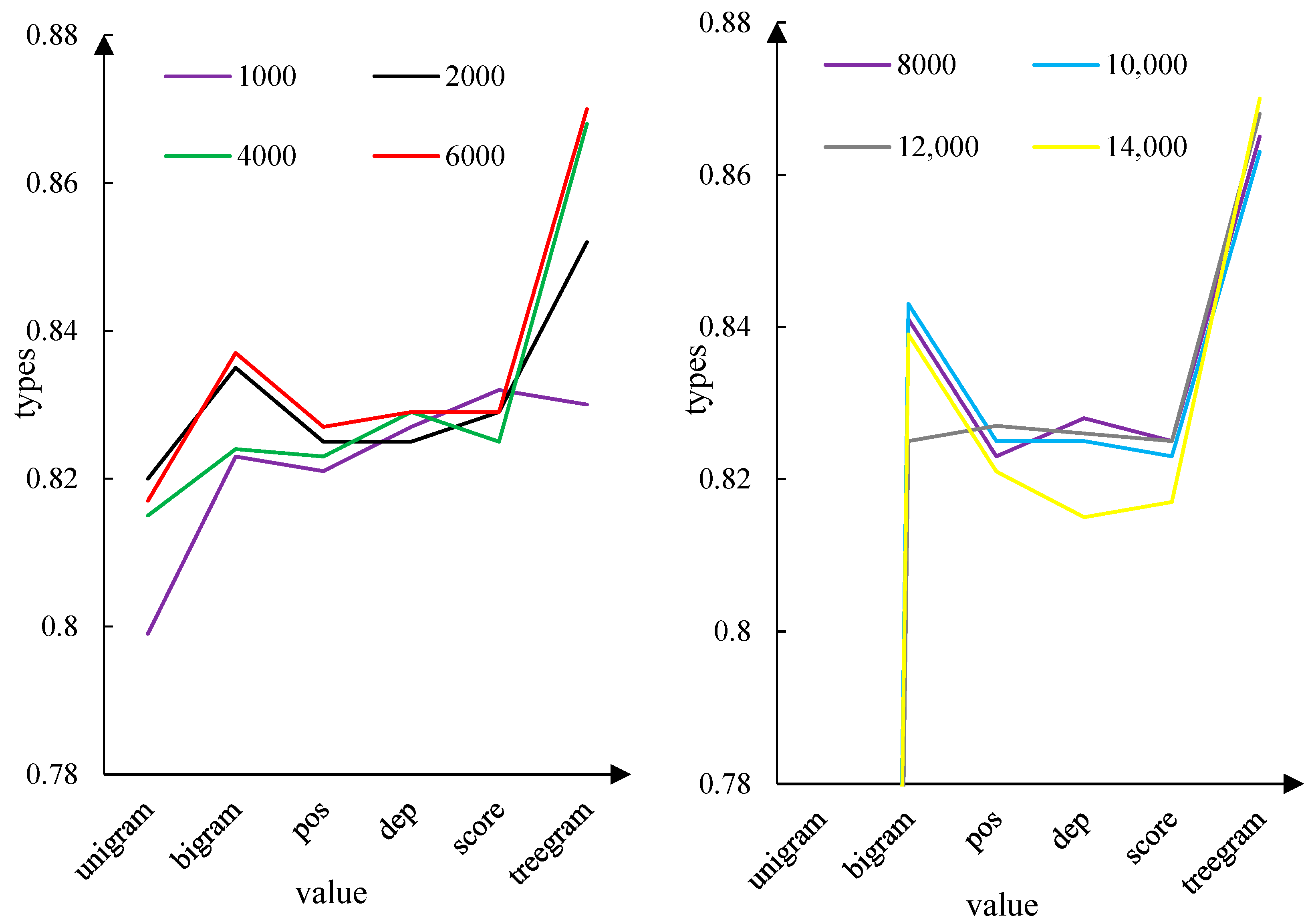
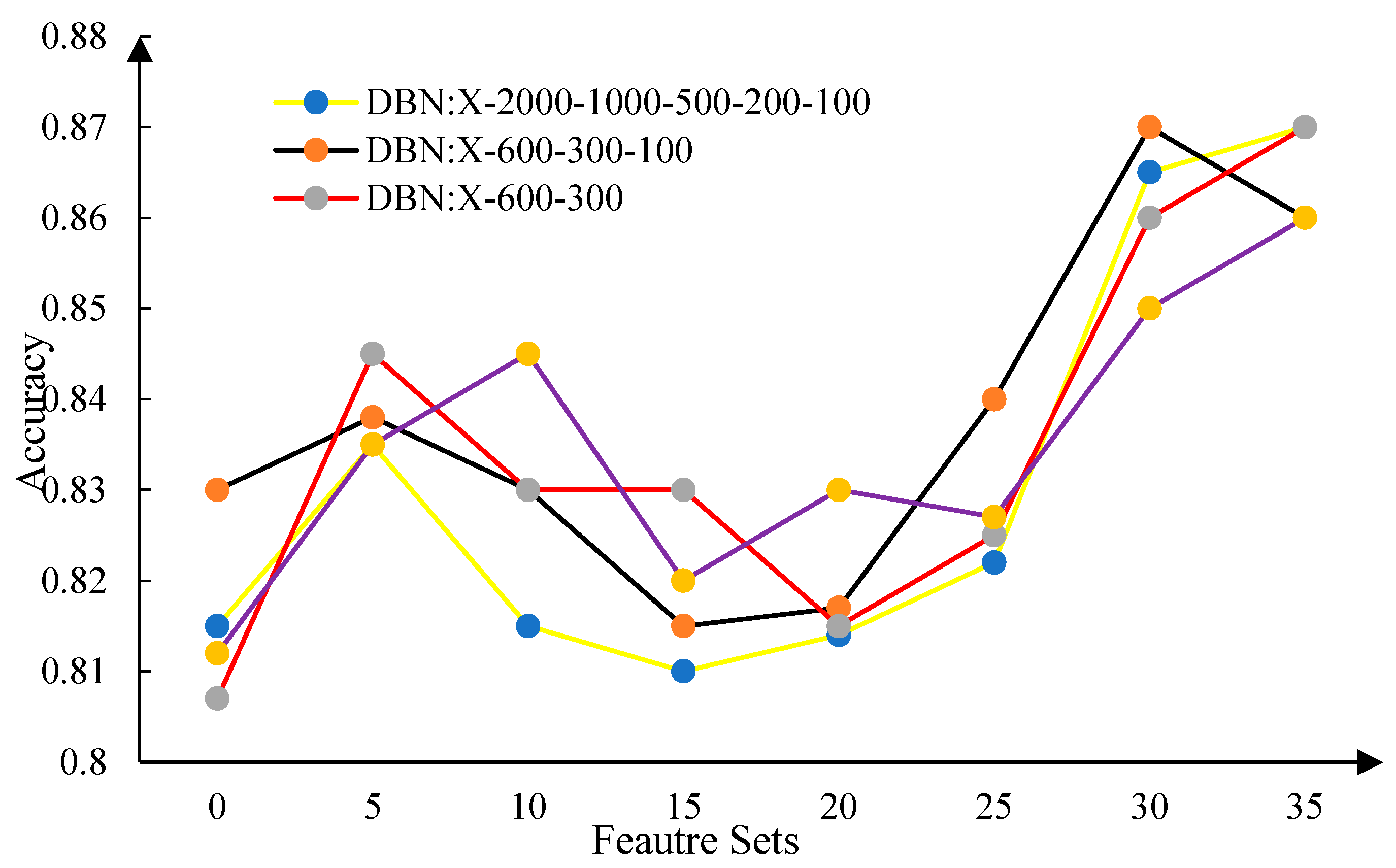
As can be seen from Figure 7, when the triplet dependency feature dimension is taken at 4000 or above, the classification accuracy exceeds other features and feature combinations. Second, the combination of monary word features achieves good classification results in some dimensions. On the basis of binary words, the classification accuracy between adding words, dependency label, and emotion score features is not very different, and the average classification accuracy of single word features is the lowest. According to the calculation, the average classification accuracy according to different feature sets is successively: 0.8106, 0.8341, 0.8272, 0.8243, 0.8272, and 0.8605. The best classification accuracy on different feature sets is 0.82, 0.8441, 0.8341, 0.8308, 0.8341, and 0.87. Conclusion DBN: X-2000-1000-500-200-100, DBN: X-600-300-100.

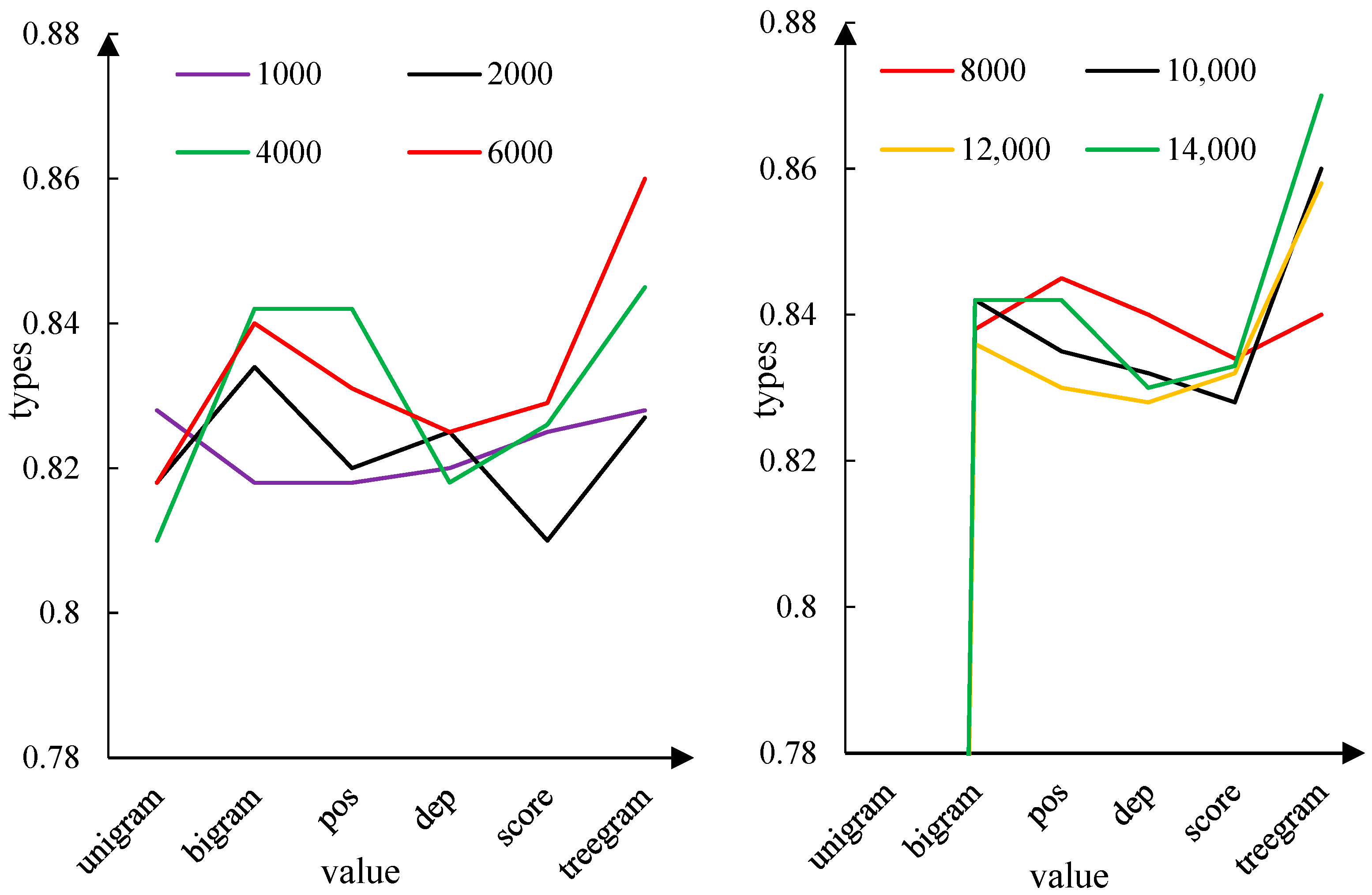
As can be seen from Figure 8, when the triplet dependency feature dimension is taken at 4000 or above, the classification accuracy exceeds other features and feature combinations. The average classification accuracy of binary word features is higher than the addition of word features, dependency labels, and emotion score. The lowest average classification accuracy was on unitary word features. According to the calculation, the average classification accuracy of different feature sets is: 0.8196, 0.8349, 0.8307, 0.8276. Meta-learning text emotion classification 850.8306, 0.8479. Based on deep belief network, the highest classification accuracy obtained was: 0.8275, 0.8416, 0.8425, 0.8375, 0.8391, and 0.8641.

(2) Analysis and comparison of deep belief network and BP network

The deep belief network is composed of the multilayered restricted Boltzmann machine in the stack form, and the initial weights of the network are learned by the restricted Boltzmann machine algorithm, and then adjusted by the BP algorithm according to the label data. However, the initial value of the network is randomly assigned, which is adjusted by the BP algorithm, which leads to the non-convergence of the BP network due to the error decline. This section analyzes the classification accuracy and convergence of deep belief networks and BP networks in experiments.

The deep belief network structure with different numbers of layers was compared with the classification accuracy of the BP networks, They are: One yuan word 4000, One Word 6000, +Binary word 4000, +Binary word 6000, +Binary word 8000, +Binary word 10,000, +Binary word 12,000, +Binary word 14,000, +Sex of Words 4000, +Sex of Words 6000, +Sex of Words 8000, +Sex of words 10,000, +Sex of Words 12,000, +Sex of Words 14,000, +Lalabel 4000, +Lalabel 6000, +Lalabel 8000, +Lalabel 10,000, +dependent label 12000, +Lalabel 14,000, +Emotional score of 4000, +5 Emotional score of 6000, +Emotional score of 8000, +Emotional score of 10,000, +Emotional Score of 12,000, +Emotional score of 14,000, Terplet dependency 4000, Terplet dependency 6000, Terplet dependency 8000, Terplet dependency 10,000, Terplet dependencies 12,000, Terplet dependency 14,000. The comparison of the obtained results is shown in Figure 9.

The structural classification accuracy of the three different deep belief networks in Figure 9 has almost the same trend at each input node. In the comparison of deep belief network and BP between the 11th node and the 26th node, BP: X-600 is better than other networks, while DBN-X-2000-1000-500-500-200-100, from the 28th to 32nd junction, BP: X-600 has the lowest classification accuracy, indicating that BP learns less under complex features, less than the deep belief network [22].

BP network algorithm is an essential gradient descent method, and the high dimensional characteristics of network input and the nature of text emotion classification itself make optimization objective function very complex, therefore, the process of “zigzag” phenomenon is used. When the optimization of neuron output is close to 0 or 1, the weight error change is small, in the error spread to pause, leading to network convergence. However, in the deep belief network, the optimization of weights is realized by limiting the Boltzmann machine to avoid the non-convergence due to too small error in the gradient descent algorithm [23].

5. Conclusions

The main work and conclusions are as follows:

(1) According to the characteristics of Chinese text, by analyzing the theory, characteristics, and generating methods of dependent syntactic relationship, yielded the process of constructing the dependent relationship characteristics of Chinese triad; it analyzed and summarized the dependent syntactic relationship of many Chinese sentences, and formulated the rules for Chinese sentences without affecting the structure of dependent tree. The merge and delete algorithm of redundancy and useless nodes are presented. The above method is used in Chinese hotel review data, book review data, and laptop review data, effectively realizing the conversion of triplet dependency characteristics of text [24,25].

(2) It compared the accuracy of text emotion classification by comparing the combination of the proposed ternary dependency features and common text representation features including monary words, binary words, words, dependency labels, and emotion scores [26,27]. To this end, two sets of experiments are designed for comparative analysis: one calculates the emotion score of each comment statement on three datasets based on semantic methods, and one uses the features extracted from three data instances for machine learning and k-neighbor classification algorithm [28]. Meanwhile, the text feature representation method of different feature sets is dimension-reduced, and the feature vector space of different dimensions is used in traditional machine learning algorithms. Experimental results show that the triplet dependent feature representation method is effective in text emotion classification, with a much higher result than the emotion dictionary scores based on semantic methods, and the classification accuracy reaches 84 to 86% in large-scale data for SVM classification algorithms, increasing 2~3% based on existing features. But it is also found that the triplet dependency feature leads to the growth of the characteristic dimension. Determining the dimension is a difficult problem to reduce the dimension. However, due to the limitations of time and technology, this paper has not carried out a detailed analysis of the problems encountered in the emotional classification of short text, which will be further discussed in the future.

References

1. Chang, G.; Huo, H. A method of fine-grained short text sentiment analysis based on machine learning. Neural Netw. World 2018, 28, 325–344. [Google Scholar] [CrossRef] [Green Version]
2. Sun, X.; Peng, X.; Hu, M. Extended Multi-modality Features and Deep Learning Based Microblog Short Text Sentiment Analysis. Dianzi Yu Xinxi Xuebao/J. Electron. Inf. Technol. 2017, 39, 2048–2055. [Google Scholar] [CrossRef]
3. Joshi, S.; Deshpande, D. Twitter Sentiment Analysis System. Int. J. Comput. Appl. 2018, 180, 35–39. [Google Scholar] [CrossRef]
4. Piryani, R.; Piryani, B.; Singh, V.K.; Pinto, D. Sentiment analysis in Nepali: Exploring machine learning and lexicon-based approaches. J. Intell. Fuzzy Syst. 2020, 39, 2201–2212. [Google Scholar] [CrossRef]
5. Attieh, J.; Tekli, J. Supervised term-category feature weighting for improved text classification. Knowl. Based Syst. 2023, 261, 110215. [Google Scholar] [CrossRef]
6. El Hindi, K.M.; Aljulaidan, R.R.; AlSalman, H. Lazy fine-tuning algorithms for naïve Bayesian text classification. Appl. Soft Comput. 2020, 96, 106652. [Google Scholar] [CrossRef]
7. Jiang, W.; Zhou, K.; Xiong, C.; Guodong, D.; Chubin, O.; Zhang, J. KSCB: A novel unsupervised method for text sentiment analysis. Appl. Intell. 2023, 53, 301–311. [Google Scholar] [CrossRef]
8. Divate, M.S. Sentiment analysis of Marathi news using LSTM. Int. J. Inf. Technol. 2021, 13, 2069–2074. [Google Scholar] [CrossRef]
9. Bhagat, C.; Mane, D. Survey On Text Categorization Using Sentiment Analysis. Int. J. Sci. Technol. Res. 2019, 8, 1189–1195. [Google Scholar]
10. Albayati, A.Q.; Al_Araji, A. Arabic Sentiment Analysis (ASA) Using Deep Learning Approach. Univ. Baghdad Eng. J. 2020, 26, 85–93. [Google Scholar] [CrossRef]
11. Ali, F.; Ali, A.; Imran, M.; Naqvi, R.A.; Siddiqi, M.H.; Kwak, K.-S. Traffic accident detection and condition analysis based on social networking data. Accid. Anal. Prev. 2021, 151, 105973. [Google Scholar] [CrossRef] [PubMed]
12. Rusnachenko, N.; Loukachevitch, N. Attention-Based Neural Networks for Sentiment Attitude Extraction using Distant Supervision. In Proceedings of the 10th International Conference on Web Intelligence, Mining and Semantics, Biarritz, France, 30 June–3 July 2020; pp. 159–168. [Google Scholar] [CrossRef]
13. Gallego, F.O.; Corchuelo, R. Torii: An aspect-based sentiment analysis system that can mine conditions. Software 2020, 50, 47–64. [Google Scholar] [CrossRef]
14. Chen, J.; Yan, S.; Wong, K.C. Verbal aggression detection on Twitter comments: Convolutional neural network for short-text sentiment analysis. Neural Comput. Appl. 2018, 3, 10809–10818. [Google Scholar] [CrossRef]
15. Rehman, A.U.; Malik, A.K.; Raza, B. A Hybrid CNN-LSTM Model for Improving Accuracy of Movie Reviews Sentiment Analysis. Multimed. Tools Appl. 2019, 78, 26597–26613. [Google Scholar] [CrossRef]
16. Karthik, E.; Sethukarasi, T. Sarcastic user behavior classification and prediction from social media data using firebug swarm optimization-based long short-term memory. J. Supercomput. 2021, 78, 5333–5357. [Google Scholar] [CrossRef]
17. Wang, X.; Zhang, H.; Xu, Z. Public Sentiments Analysis Based on Fuzzy Logic for Text. Int. J. Softw. Eng. Knowl. Eng. 2016, 26, 1341–1360. [Google Scholar] [CrossRef]
18. Ashok, K.J.; Trueman, T.E.; Cambria, E. A Convolutional Stacked Bidirectional LSTM with a Multiplicative Attention Mechanism for Aspect Category and Sentiment Detection. Cogn. Comput. 2021, 13, 1423–1432. [Google Scholar]
19. Roseline, V.; Chellam, G.H. Sentiment Classification Using PS-POS Embedding with Bilstm-CRF and Attention. Int. J. Future Gener. Commun. Netw. 2020, 13, 3520–3526. [Google Scholar]
20. Han, H.; Bai, X.; Ping, L. Augmented sentiment representation by learning context information. Neural Comput. Appl. 2019, 31, 8475–8482. [Google Scholar] [CrossRef]
21. Sengan, S.P.; Sagar, V.; Khalaf, O.I.; Dhanapal, R. The optimization of reconfigured real-time datasets for improving classification performance of machine learning algorithms. Math. Eng. Sci. Aerosp. 2021, 12, 43–54. [Google Scholar]
22. Roseline, V.; Herenchellam, D. PS-POS Embedding Target Extraction Using CRF and BiLSTM. Int. J. Adv. Sci. Technol. 2020, 29, 10984–10995. [Google Scholar]
23. Bashar, M.A.; Nayak, R.; Luong, K. Progressive domain adaptation for detecting hate speech on social media with small training set and its application to COVID-19 concerned posts. Soc. Netw. Anal. Min. 2021, 11, 69. [Google Scholar] [CrossRef] [PubMed]
24. Huan, J.L.; Sekh, A.A.; Quek, C.; Prasad, D.K. Emotionally charged text classification with deep learning and sentiment semantic. Neural Comput. Appl. 2021, 34, 2341–2351. [Google Scholar] [CrossRef]
25. Yan, Z.; Cao, W.; Ji, J. Social behavior prediction with graph U-Net+. Discov. Internet Things 2021, 1, 18. [Google Scholar] [CrossRef]
26. Brooke, J.; Hammond, A.; Hirst, G. Using models of lexical style to quantify free indirect discourse in modernist fiction. Lit. Linguist. Comput. 2017, 32, 234–250. [Google Scholar] [CrossRef] [Green Version]
27. Kumar, M.; Aggarwal, J.; Rani, A.; Stephan, T.; Shankar, A.; Mirjalili, S. Secure video communication using firefly optimization and visual cryptography. Artif. Intell. Rev. 2021, 55, 2997–3017. [Google Scholar] [CrossRef]
28. Lu, H.; Wang, S.S.; Zhou, Q.W.; Zhao, Y.N.; Zhao, B.Y. Damage and control of major poisonous plants in the western grasslands of China? a review. Rangel. J. 2012, 34, 329. [Google Scholar] [CrossRef]
Figure 1. Overall framework.
Electronics 12 01589 g001
Figure 2. Bayesian network structure diagram.
Electronics 12 01589 g002
Figure 3. BR-DBN model structure.
Electronics 12 01589 g003
Figure 4. Flow chart of emotion classification.
Electronics 12 01589 g004
Figure 5. DBN: X20000-1000-500-200-100 classification standard rate.
Electronics 12 01589 g005
Figure 6. DBN: X600-300-100 classification standard rate.
Electronics 12 01589 g006
Figure 7. DBN: X600-300 classification standard rate.
Electronics 12 01589 g007
Figure 8. DBN: X600 classification standard rate.
Electronics 12 01589 g008
Figure 9. Emotional analysis line chart.
Electronics 12 01589 g009