
Dynamic Optimal Power Flow of Active Distribution Network Based on LSOCR and Its Application Scenarios

 ,
,  ,
, 
 and
and 
Abstract
1. Introduction
- (1)
- (2)
- Approximation of power flow equality constraints. For example, the AC-OPF constraints can be approximately linearized as direct current power flow constraints, and the resultant direct current optimal power flow (DC-OPF) problem can be accordingly solved [9];
- (3)
- Relaxation of the power flow equality constraint using convex relaxation techniques [10].
- Present the LSOCR-DOPF model, which is based on branch power flow analysis, for the active distribution network.
- Explore the linear modeling method for the constraints of various active management units, including OLTC, SVC, CB, ESS, etc.
- Validate the LSOCR-DOPF model through simulation experiments in three typical scenarios: power coordination optimization, network reconfiguration, and ZIP load application.
2. Methodology
2.1. LSOCR-DOPF Model of the Distribution Network
2.1.1. Basic Structure of Distribution Networks
2.1.2. Basic OPF Model Based on BFM
2.1.3. Multi-Period LSOCR-OPF Model
2.2. Active Distribution Network Modeling
2.2.1. Active Distribution Network Units Modeling
- 1.
- Active power regulation device
- (1)
- Modeling of discrete reactive power compensation (CB).where, is the set of nodes; is the number of groups put into operation and the discrete variable value; is the upper limit of the number of groups connected by node ; is the compensation power of each group of . Considering factors such as equipment life or economy, discrete reactive compensation is mostly limited by the number of adjustments, so it generally includes the total number of operations in multiple periods; is the upper limit of operation times:In addition, for the absolute value constraint in the above equation, add an auxiliary variable that represents the change in CB compensation capacity between adjacent periods, corresponding to:
- (2)
- Modeling of continuous reactive power regulation device (SVC).where, is the node set containing ; and are the lower limit and upper limit of compensation power, respectively. Considering that, in the process of active distribution network operation, with the increasing penetration of distributed generation (DG) such as photovoltaic power generation, the system power flow may be reversed and overvoltage problems may occur, the lower limit of compensation in this paper is: .
- 2.
- OLTC modelThe OLTC is used to adjust the voltage value at the low-voltage side of the bus node. Therefore, the substation bus node is further converted to the adjustable variable:where, refers to the node set of substation containing OLTC; is the voltage value at the high voltage side of the transformer, which is a constant value; and are the square of the upper and lower limit of the OLTC adjustable transformation ratio; is the square of the OLTC transformation ratio, defined as the ratio of the secondary side to the primary side, which is actually a discrete value variable, and can be further treated as the following relationship including 0–1 variables:where, represents the difference between OLTC gear and the square of gear , which is the adjacent adjustment increment. is a 0–1 identification variable. If it is considered to be constrained by the limit of adjustment times in practice, it can be further constrained as:where, and represent the OLTC gear adjustment change sign, which is 0–1 variable; if , then the gear value of OLTC at time − 1 is greater than the gear value at time , is similar; is the maximum range of gear change; is the maximum allowable adjustment times of the OLTC gear at time .
- 3.
- ESS modelDuring this part, the modeling of the energy storage system takes into account multiple-period constraints, including restrictions on its charging and discharging status, charging and discharging power, as well as capacity limitations.
- (1)
- Power limit.
- (2)
- Charge and discharge status limit.
- (3)
- Capacity constraints.where, is the node set containing ; Equation (23) indicates that the cannot be simultaneously charged and discharged at the same time, and is and are the upper and lower limits of charging and discharging power, respectively; is the power of the t period of , and are the upper and lower limit values considering factors such as life; and are the charge and discharge efficiency coefficient, respectively, generally , .As a novel active management technique, electric vehicles can be considered as mobile active power energy storage systems [33]. Their basic model is largely similar to that of Energy Storage Systems (ESS). The equivalent injection power at each bus node in the distribution network can be represented as the clustering outcomes of individual electric vehicles.
- 4.
- Distributed generation modelRespectively modeling with or without reactive power:
- (1)
- modeling without considering reactive power.Currently, the modeling form of active management for DG primarily takes into account the possibility of DG allowing power shedding under certain conditions, and assumes that DG is only related to active power output [34], that is:where, is the node set containing ; is the predicted active power output of node at time .
- (2)
- modeling considering reactive power [35].With the maturity of active power regulation as a primary method in the study of DG and the advent of new technology, some DGs can have a certain impact on reactive power in the power grid, including outputting and absorbing reactive power. As a result, active management research focusing on the reactive power of DG has emerged, mainly divided into constant power factor control and variable power factor control.
- ①
- Constant power factor control
- ②
- Variable power factor controlwhere, and are the upper and lower limits of transformation ratio adjustment; represents the ratio of reactive power to active power, and its optimization range can be converted from the power factor control range. At present, most of the literature will limit the reactive power and is set as a constant [27].
2.2.2. Radial Constraints
2.2.3. ZIP Load Application
2.3. Proposed LSOCR-DOPF Optimization Flowchart
3. Validation and Discussions
3.1. Power Coordination Optimization
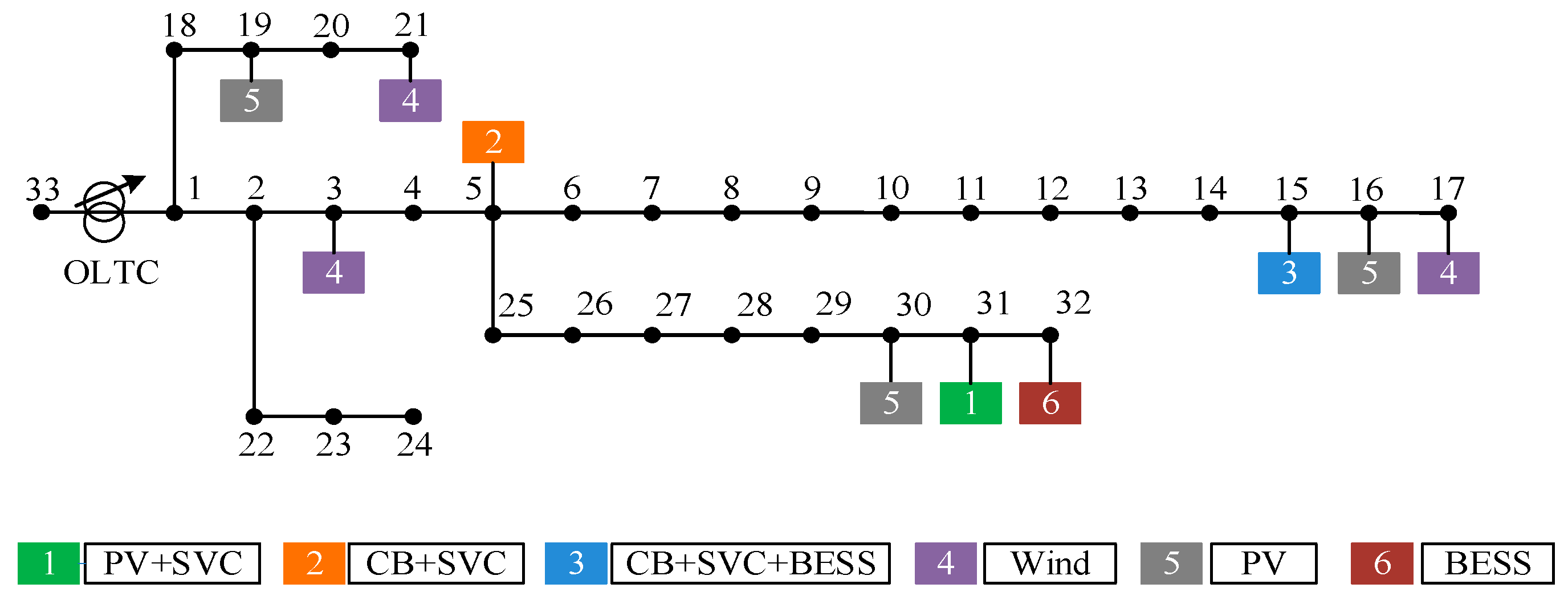
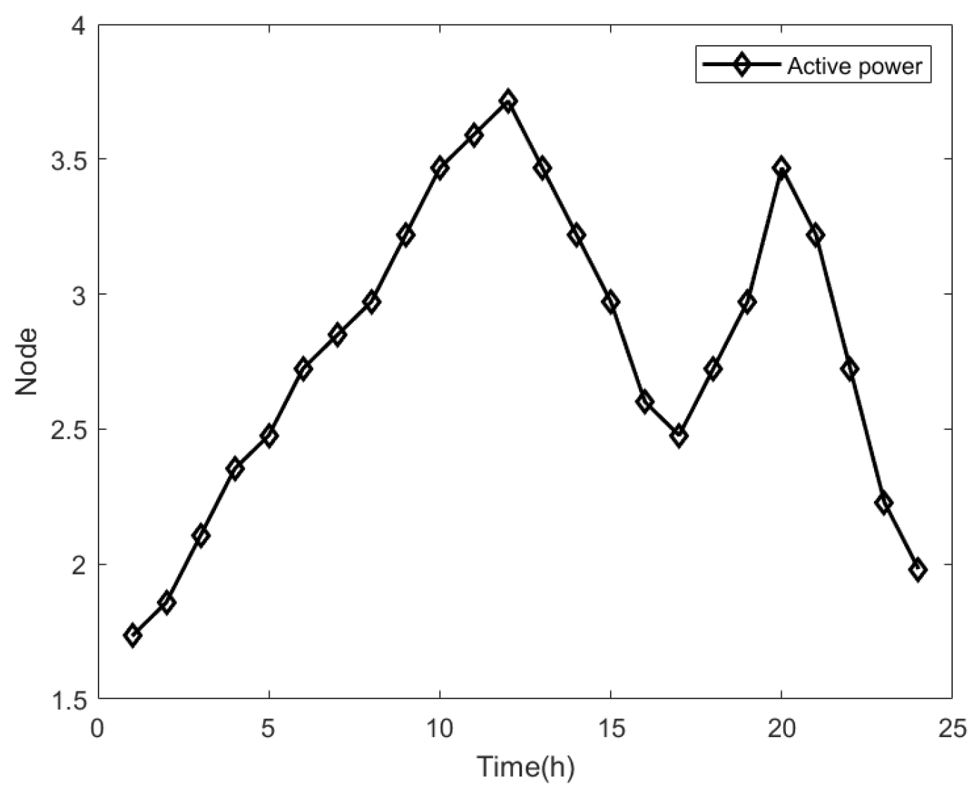
3.1.1. Scenario Description
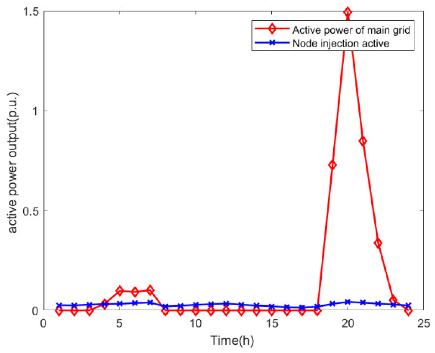
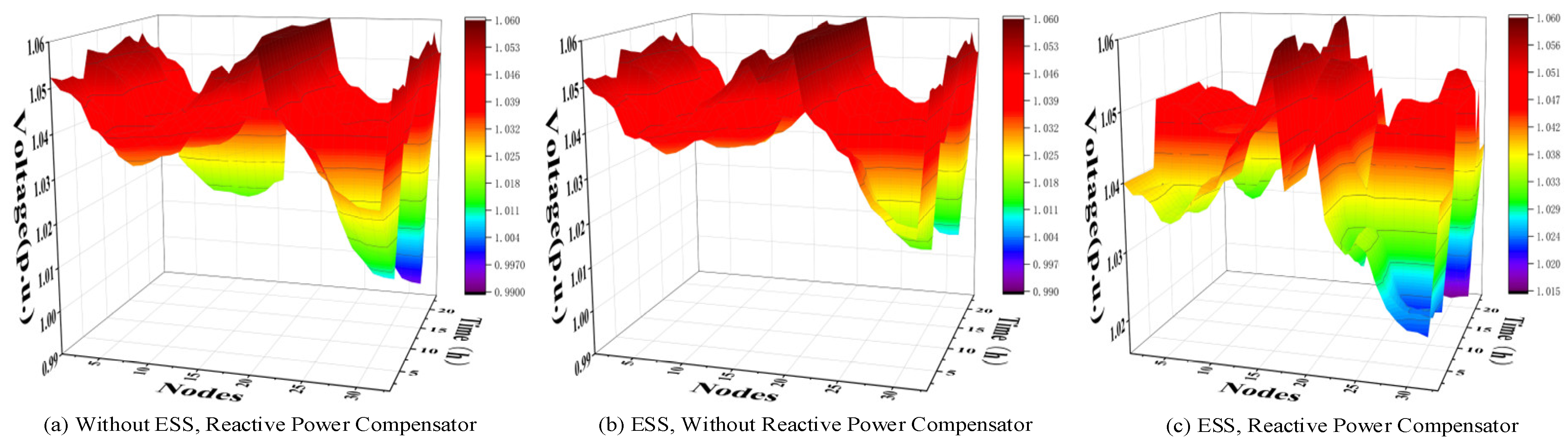
3.1.2. Analysis of Optimization Results
3.1.3. Model Validity Analysis
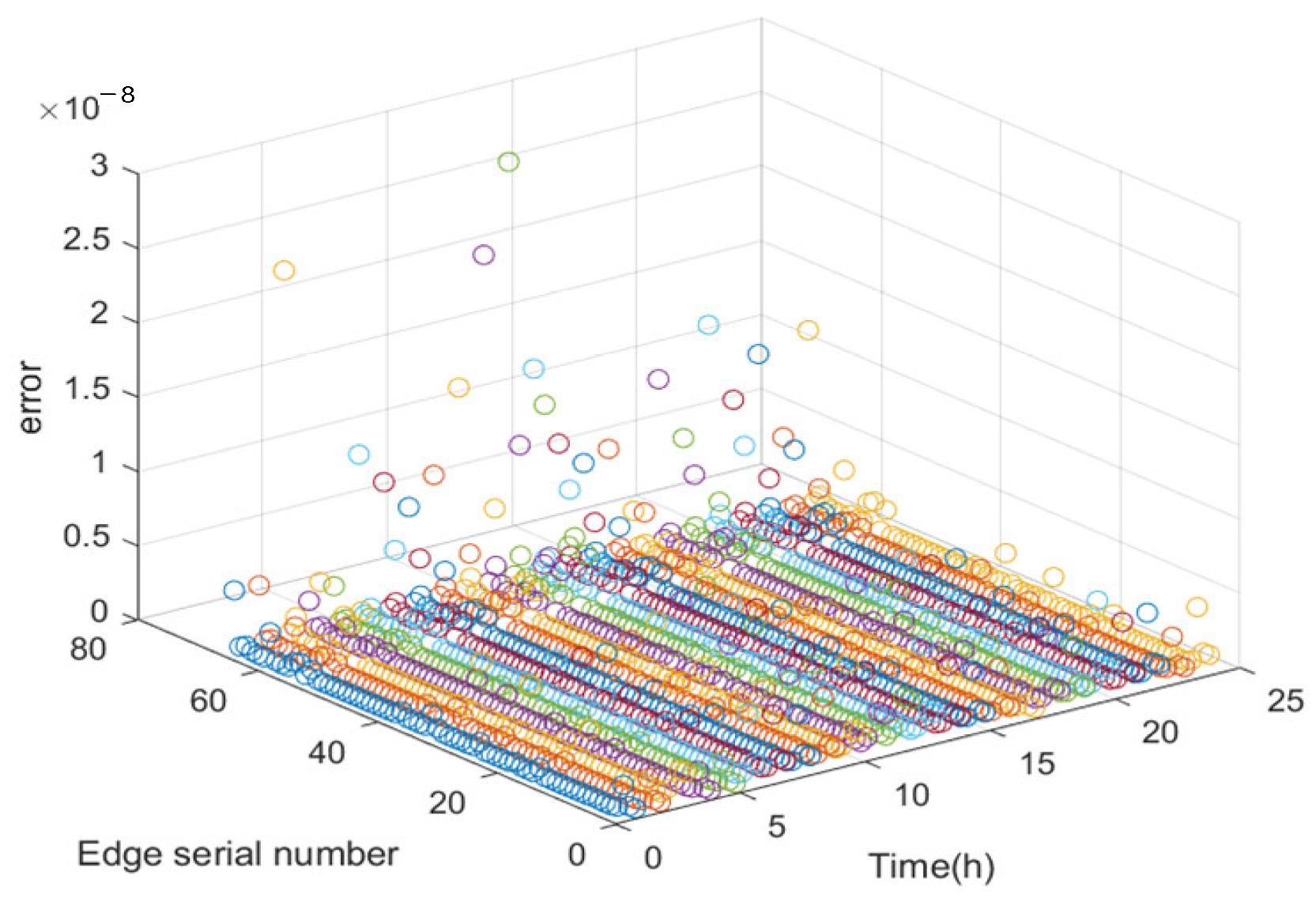
- (1)
- Relaxation accuracy
- (2)
- Calculation timeliness
- (3)
- Comparison of different optimization cases
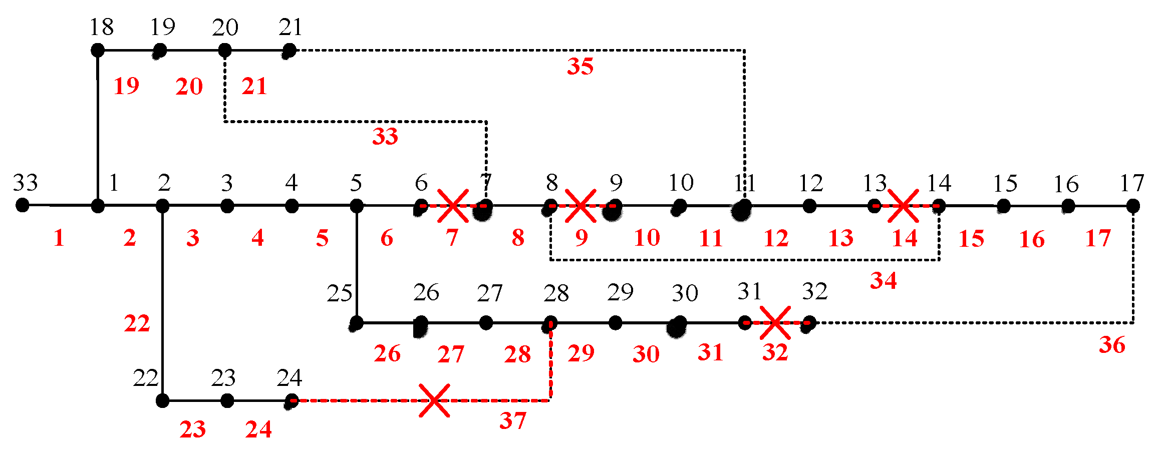
3.2. Network Reconfiguration
3.3. ZIP Load Application
4. Conclusions
Author Contributions
Funding
Data Availability Statement
Conflicts of Interest
Appendix A


| Branch Number | Sending Bus | Receiving Bus | Resistance Ω | Reactance Ω | Nominal Load at Receiving Bus | Maximum Line Capacity (kVA) | |
|---|---|---|---|---|---|---|---|
| P (kW) | Q(kVA) | ||||||
| 1 | 1 | 2 | 0.0005 | 0.0012 | 0.0 | 0.0 | 10,761 |
| 2 | 2 | 3 | 0.0005 | 0.0012 | 0.0 | 0.0 | 10,761 |
| 3 | 3 | 4 | 0.0015 | 0.0036 | 0.0 | 0.0 | 10,761 |
| 4 | 4 | 5 | 0.0251 | 0.0294 | 0.0 | 0.0 | 5823 |
| 5 | 5 | 6 | 0.3660 | 0.1864 | 2.60 | 2.20 | 1899 |
| 6 | 6 | 7 | 0.3811 | 0.1941 | 40.40 | 30.00 | 1899 |
| 7 | 7 | 8 | 0.0922 | 0.0470 | 75.00 | 54.00 | 1899 |
| 8 | 8 | 9 | 0.0493 | 0.0251 | 30.00 | 22.00 | 1899 |
| 9 | 9 | 10 | 0.8190 | 0.2707 | 28.00 | 19.00 | 1455 |
| 10 | 10 | 11 | 0.1872 | 0.0619 | 145.00 | 104.00 | 1455 |
| 11 | 11 | 12 | 0.7114 | 0.2351 | 145.00 | 104.00 | 1455 |
| 12 | 12 | 13 | 1.0300 | 0.3400 | 8.00 | 5.00 | 1455 |
| 13 | 13 | 14 | 1.0440 | 0.3450 | 8.00 | 5.50 | 1455 |
| 14 | 14 | 15 | 1.0580 | 0.3496 | 0.0 | 0.0 | 1455 |
| 15 | 15 | 16 | 0.1966 | 0.0650 | 45.50 | 30.00 | 1455 |
| 16 | 16 | 17 | 0.3744 | 0.1238 | 60.00 | 35.00 | 1455 |
| 17 | 17 | 18 | 0.0047 | 0.0016 | 60.00 | 35.00 | 2200 |
| 18 | 18 | 19 | 0.3276 | 0.1083 | 0.0 | 0.0 | 1455 |
| 19 | 19 | 20 | 0.2106 | 0.0690 | 1.00 | 0.60 | 1455 |
| 20 | 20 | 21 | 0.3416 | 0.1129 | 114.00 | 81.00 | 1455 |
| 21 | 21 | 22 | 0.0140 | 0.0046 | 5.00 | 3.50 | 1455 |
| 22 | 22 | 23 | 0.1591 | 0.0526 | 0.0 | 0.0 | 1455 |
| 23 | 23 | 24 | 0.3463 | 0.1145 | 28.00 | 20.0 | 1455 |
| 24 | 24 | 25 | 0.7488 | 0.2475 | 0.0 | 0.0 | 1455 |
| 25 | 25 | 26 | 0.3089 | 0.1021 | 14.0 | 10.0 | 1455 |
| 26 | 26 | 27 | 0.1732 | 0.0572 | 14.0 | 10.0 | 1455 |
| 27 | 3 | 28 | 0.0044 | 0.0108 | 26.0 | 18.6 | 10,761 |
| 28 | 28 | 29 | 0.0640 | 0.1565 | 26.0 | 18.6 | 10,761 |
| 29 | 29 | 30 | 0.3978 | 0.1315 | 0.0 | 0.0 | 1455 |
| 30 | 30 | 31 | 0.0702 | 0.0232 | 0.0 | 0.0 | 1455 |
| 31 | 31 | 32 | 0.3510 | 0.1160 | 0.0 | 0.0 | 1455 |
| 32 | 32 | 33 | 0.8390 | 0.2816 | 14.0 | 10.0 | 2200 |
| 33 | 33 | 34 | 1.7080 | 0.5646 | 9.50 | 14.00 | 1455 |
| 34 | 34 | 35 | 1.4740 | 0.4873 | 6.00 | 4.00 | 1455 |
| 35 | 3 | 36 | 0.0044 | 0.0108 | 26.0 | 18.55 | 10,761 |
| 36 | 36 | 37 | 0.0640 | 0.1565 | 26.0 | 18.55 | 10,761 |
| 37 | 37 | 38 | 0.1053 | 0.1230 | 0.0 | 0.0 | 5823 |
| 38 | 38 | 39 | 0.0304 | 0.0355 | 24.0 | 17.00 | 5823 |
| 39 | 39 | 40 | 0.0018 | 0.0021 | 24.0 | 17.00 | 5823 |
| 40 | 40 | 41 | 0.7283 | 0.8509 | 1.20 | 1.0 | 5823 |
| 41 | 41 | 42 | 0.3100 | 0.3623 | 0.0 | 0.0 | 5823 |
| 42 | 42 | 43 | 0.0410 | 0.0478 | 6.0 | 4.30 | 5823 |
| 43 | 43 | 44 | 0.0092 | 0.0116 | 0.0 | 0.0 | 5823 |
| 44 | 44 | 45 | 0.1089 | 0.1373 | 39.22 | 26.30 | 5823 |
| 45 | 45 | 46 | 0.0009 | 0.0012 | 39.22 | 26.30 | 6709 |
| 46 | 4 | 47 | 0.0034 | 0.0084 | 0.00 | 0.0 | 10,761 |
| 47 | 47 | 48 | 0.0851 | 0.2083 | 79.00 | 56.40 | 10,761 |
| 48 | 48 | 49 | 0.2898 | 0.7091 | 384.70 | 274.50 | 10,761 |
| 49 | 49 | 50 | 0.0822 | 0.2011 | 384.70 | 274.50 | 10,761 |
| 50 | 8 | 51 | 0.0928 | 0.0473 | 40.50 | 28.30 | 1899 |
| 51 | 51 | 52 | 0.3319 | 0.1114 | 3.60 | 2.70 | 2200 |
| 52 | 52 | 53 | 0.1740 | 0.0886 | 4.35 | 3.50 | 1899 |
| 53 | 53 | 54 | 0.2030 | 0.1034 | 26.40 | 19.00 | 1899 |
| 54 | 54 | 55 | 0.2842 | 0.1447 | 24.00 | 17.20 | 1899 |
| 55 | 55 | 56 | 0.2813 | 0.1433 | 0.0 | 0.0 | 1899 |
| 56 | 56 | 57 | 1.5900 | 0.5337 | 0.0 | 0.0 | 2200 |
| 57 | 57 | 58 | 0.7837 | 0.2630 | 0.0 | 0.0 | 2200 |
| 58 | 58 | 59 | 0.3042 | 0.1006 | 100.0 | 72.0 | 1455 |
| 59 | 59 | 60 | 0.3861 | 0.1172 | 0.0 | 0.0 | 1455 |
| 60 | 60 | 61 | 0.5075 | 0.2585 | 1244.0 | 888.00 | 1899 |
| 61 | 61 | 62 | 0.0974 | 0.0496 | 32.0 | 23.00 | 1899 |
| 62 | 62 | 63 | 0.1450 | 0.0738 | 0.0 | 0.0 | 1899 |
| 63 | 63 | 64 | 0.7105 | 0.3619 | 227.0 | 162.00 | 1899 |
| 64 | 64 | 65 | 1.0410 | 0.5302 | 59.0 | 42.0 | 1899 |
| 65 | 11 | 66 | 0.2012 | 0.0611 | 18.0 | 13.0 | 1455 |
| 66 | 66 | 67 | 0.0047 | 0.0014 | 18.0 | 13.0 | 1455 |
| 67 | 12 | 68 | 0.7394 | 0.2444 | 28.0 | 20.0 | 1455 |
| 68 | 68 | 69 | 0.0047 | 0.0016 | 28.0 | 20.0 | 1455 |
| 69 * | 11 | 43 | 0.5000 | 0.5000 | 566 | ||
| 70 * | 13 | 21 | 0.5 | 0.5 | 566 | ||
| 71 * | 15 | 46 | 1.0 | 1.0 | 400 | ||
| 72 * | 50 | 59 | 2.0 | 2.0 | 283 | ||
| 73 * | 27 | 65 | 1.0 | 1.0 | 400 | ||
| Branch Number | Sending Bus | Receiving Bus | Resistance Ω | Reactance Ω | Nominal Load at Receiving Bus | |
|---|---|---|---|---|---|---|
| P (kW) | Q (kVA) | |||||
| 1 | 1 | 2 | 0.0922 | 0.047 | 100 | 60 |
| 2 | 2 | 3 | 0.493 | 0.2511 | 90 | 40 |
| 3 | 3 | 4 | 0.366 | 0.1864 | 120 | 80 |
| 4 | 4 | 5 | 0.3811 | 0.1941 | 60 | 30 |
| 5 | 5 | 6 | 0.819 | 0.707 | 60 | 20 |
| 6 | 6 | 7 | 0.1872 | 0.6188 | 200 | 100 |
| 7 | 7 | 8 | 0.7114 | 0.2351 | 200 | 100 |
| 8 | 8 | 9 | 1.03 | 0.74 | 60 | 20 |
| 9 | 9 | 10 | 1.044 | 0.74 | 60 | 20 |
| 10 | 10 | 11 | 0.1966 | 0.065 | 45 | 30 |
| 11 | 11 | 12 | 0.3744 | 0.1298 | 60 | 35 |
| 12 | 12 | 13 | 1.468 | 1.155 | 60 | 35 |
| 13 | 13 | 14 | 0.5416 | 0.7129 | 120 | 80 |
| 14 | 14 | 15 | 0.591 | 0.526 | 60 | 10 |
| 15 | 15 | 16 | 0.7463 | 0.545 | 60 | 20 |
| 16 | 16 | 17 | 1.289 | 1.721 | 60 | 20 |
| 17 | 17 | 18 | 0.732 | 0.574 | 90 | 40 |
| 18 | 2 | 19 | 0.164 | 0.1565 | 90 | 40 |
| 19 | 19 | 20 | 1.5042 | 1.3554 | 90 | 40 |
| 20 | 20 | 21 | 0.4095 | 0.4784 | 90 | 40 |
| 21 | 21 | 22 | 0.7089 | 0.9373 | 90 | 40 |
| 22 | 3 | 23 | 0.4512 | 0.3083 | 90 | 50 |
| 23 | 23 | 24 | 0.898 | 0.7091 | 420 | 200 |
| 24 | 24 | 25 | 0.896 | 0.7011 | 420 | 200 |
| 25 | 6 | 26 | 0.203 | 0.1034 | 60 | 25 |
| 26 | 26 | 27 | 0.2842 | 0.1447 | 60 | 25 |
| 27 | 27 | 28 | 1.059 | 0.9337 | 60 | 20 |
| 28 | 28 | 29 | 0.8042 | 0.7006 | 120 | 70 |
| 29 | 29 | 30 | 0.5075 | 0.2585 | 200 | 600 |
| 30 | 30 | 31 | 0.9744 | 0.963 | 150 | 70 |
| 31 | 31 | 32 | 0.3105 | 0.3619 | 210 | 100 |
| 32 | 32 | 33 | 0.341 | 0.5302 | 60 | 40 |
| 33 | 20 | 7 | 2.0000 | 2.0000 | - | - |
| 34 | 8 | 14 | 2.0000 | 2.0000 | - | - |
| 35 | 11 | 21 | 2.0000 | 2.0000 | - | - |
| 36 | 17 | 32 | 0.5000 | 0.5000 | - | - |
| 37 | 24 | 28 | 0.5000 | 0.5000 | - | - |
References
- Kryonidis, G.C.; Kontis, E.O.; Papadopoulos, T.A.; Pippi, K.D.; Nousdilis, A.I.; Barzegkar-Ntovom, G.A.; Boubaris, A.D.; Papanikolaou, N.P. Ancillary services in active distribution networks: A review of technological trends from operational and online analysis perspective. Renew. Sustain. Energy Rev. 2021, 147, 111198. [Google Scholar] [CrossRef]
- Davarzani, S.; Pisica, I.; Taylor, G.A.; Munisami, K.J. Residential Demand Response Strategies and Applications in Active Distribution Network Management. Renew. Sustain. Energy Rev. 2021, 138, 110567. [Google Scholar] [CrossRef]
- Papadimitrakis, M.; Giamarelos, N.; Stogiannos, M.; Zois, E.N.; Livanos, N.A.I.; Alexandridis, A. Metaheuristic search in smart grid: A review with emphasis on planning, scheduling and power flow optimization applications. Renew. Sustain. Energy Rev. 2021, 145, 111072. [Google Scholar] [CrossRef]
- Song, D.; Meng, W.; Dong, M.; Yang, J.; Wang, J.; Chen, X.; Huang, L. A critical survey of integrated energy system: Summaries, methodologies and analysis. Energy Convers. Manag. 2022, 266, 115863. [Google Scholar] [CrossRef]
- Bienstock, D.; Verma, A. Strong NP-hardness of AC power flows feasibility. Oper. Res. Lett. 2019, 47, 494–501. [Google Scholar] [CrossRef]
- Lehmann, K.; Grastien, A.; Van Hentenryck, P. AC-feasibility on tree networks is NP-hard. IEEE Trans. Power Syst. 2015, 31, 798–801. [Google Scholar] [CrossRef]
- Castillo, A.; O’Neill, R. Survey of Approaches to Solving the ACOPF: Optimal Power Flow Paper 4; FERC Staff Technical Paper: Washington, DC, USA, 2013; p. 1.
- Song, D.; Yan, J.; Zeng, H.; Deng, X.; Yang, J.; Qu, X.; Rizk-Allah, R.M.; Snášel, V.; Joo, Y.H. Topological Optimization of an Offshore-Wind-Farm Power Collection System Based on a Hybrid Optimization Methodology. J. Mar. Sci. Eng. 2023, 11, 279. [Google Scholar] [CrossRef]
- Stott, B.; Jardim, J.; Alsaç, O. DC power flow revisited. IEEE Trans. Power Syst. 2009, 24, 1290–1300. [Google Scholar] [CrossRef]
- Taylor, J.A. Convex Optimization of Power Systems; Cambridge University Press: Cambridge, UK, 2015. [Google Scholar]
- Makhadmeh, S.N.; Khader, A.T.; Al-Betar, M.A.; Naim, S.; Abasi, A.K.; Alyasseri, Z.A.A. Optimization methods for power scheduling problems in smart home: Survey. Renew. Sustain. Energy Rev. 2019, 115, 109362. [Google Scholar] [CrossRef]
- Baker, K. Solutions of DC OPF are never AC feasible. In Proceedings of the Twelfth ACM International Conference on Future Energy Systems, Online, 28 June–2 July 2021; pp. 264–268. [Google Scholar]
- Farivar, M.; Low, S.H. Branch Flow Model: Relaxations and Convexification—Part II. IEEE Trans. Power Syst. 2013, 28, 2565–2572. [Google Scholar] [CrossRef]
- Farivar, M.; Low, S.H. Branch flow model: Relaxations and convexification—Part I. IEEE Trans. Power Syst. 2013, 28, 2554–2564. [Google Scholar] [CrossRef]
- Baran, M.E.; Wu, F.F. Network reconfiguration in distribution systems for loss reduction and load balancing. IEEE Trans. Power Deliv. 1989, 4, 1401–1407. [Google Scholar] [CrossRef]
- Low, S.H. Convex relaxation of optimal power flow—Part I: Formulations and equivalence. IEEE Trans. Control Netw. Syst. 2014, 1, 15–27. [Google Scholar] [CrossRef]
- Low, S.H. Convex relaxation of optimal power flow—Part II: Exactness. IEEE Trans. Control Netw. Syst. 2014, 1, 177–189. [Google Scholar] [CrossRef]
- Gan, L.; Li, N.; Topcu, U.; Low, S.H. Exact convex relaxation of optimal power flow in radial networks. IEEE Trans. Autom. Control 2014, 60, 72–87. [Google Scholar] [CrossRef]
- Nick, M.; Cherkaoui, R.; Le Boudec, J.-Y.; Paolone, M. An exact convex formulation of the optimal power flow in radial distribution networks including transverse components. IEEE Trans. Autom. Control 2017, 63, 682–697. [Google Scholar] [CrossRef]
- Christakou, K.; Tomozei, D.-C.; Le Boudec, J.-Y.; Paolone, M. AC OPF in radial distribution networks—Part I: On the limits of the branch flow convexification and the alternating direction method of multipliers. Electr. Power Syst. Res. 2017, 143, 438–450. [Google Scholar] [CrossRef]
- Kayacık, S.E.; Kocuk, B. An MISOCP-Based Solution Approach to the Reactive Optimal Power Flow Problem. IEEE Trans. Power Syst. 2021, 36, 529–532. [Google Scholar] [CrossRef]
- Ben-Tal, A.; Nemirovski, A. On polyhedral approximations of the second-order cone. Math. Oper. Res. 2001, 26, 193–205. [Google Scholar] [CrossRef]
- Lubin, M.; Yamangil, E.; Bent, R.; Vielma, J.P. Polyhedral approximation in mixed-integer convex optimization. Math. Program. 2018, 172, 139–168. [Google Scholar] [CrossRef]
- Ferreira, R.S.; Borges, C.L.T.; Pereira, M.V. A flexible mixed-integer linear programming approach to the AC optimal power flow in distribution systems. IEEE Trans. Power Syst. 2014, 29, 2447–2459. [Google Scholar] [CrossRef]
- Garces, A. A quadratic approximation for the optimal power flow in power distribution systems. Electr. Power Syst. Res. 2016, 130, 222–229. [Google Scholar] [CrossRef]
- Ehsan, A.; Yang, Q. State-of-the-art techniques for modelling of uncertainties in active distribution network planning: A review. Appl. Energy 2019, 239, 1509–1523. [Google Scholar] [CrossRef]
- Zografou-Barredo, N.-M.; Patsios, C.; Sarantakos, I.; Davison, P.; Walker, S.L.; Taylor, P.C. MicroGrid resilience-oriented scheduling: A robust MISOCP model. IEEE Trans. Smart Grid 2020, 12, 1867–1879. [Google Scholar] [CrossRef]
- Fathi, R.; Tousi, B.; Galvani, S. Allocation of renewable resources with radial distribution network reconfiguration using improved salp swarm algorithm. Appl. Soft Comput. 2023, 132, 109828. [Google Scholar] [CrossRef]
- Ding, T.; Liu, S.; Yuan, W.; Bie, Z.; Zeng, B. A two-stage robust reactive power optimization considering uncertain wind power integration in active distribution networks. IEEE Trans. Sustain. Energy 2015, 7, 301–311. [Google Scholar] [CrossRef]
- Baran, M.E.; Wu, F.F. Optimal capacitor placement on radial distribution systems. IEEE Trans. Power Deliv. 1989, 4, 725–734. [Google Scholar] [CrossRef]
- Li, N.; Chen, L.; Low, S.H. Exact convex relaxation of OPF for radial networks using branch flow model. In Proceedings of the 2012 IEEE Third International Conference on Smart Grid Communications (SmartGridComm), Tainan, Taiwan, 5–8 November 2012; pp. 7–12. [Google Scholar]
- Mishra, D.K.; Ghadi, M.J.; Azizivahed, A.; Li, L.; Zhang, J. A review on resilience studies in active distribution systems. Renew. Sustain. Energy Rev. 2021, 135, 110201. [Google Scholar] [CrossRef]
- He, L.; Yang, J.; Yan, J.; Tang, Y.; He, H. A bi-layer optimization based temporal and spatial scheduling for large-scale electric vehicles. Appl. Energy 2016, 168, 179–192. [Google Scholar] [CrossRef]
- Xiang, Y.; Liu, J.; Liu, Y. Optimal active distribution system management considering aggregated plug-in electric vehicles. Electr. Power Syst. Res. 2016, 131, 105–115. [Google Scholar] [CrossRef]
- Das, T.; Roy, R.; Mandal, K. Impact of the penetration of distributed generation on optimal reactive power dispatch. Prot. Control. Mod. Power Syst. 2020, 5, 31. [Google Scholar] [CrossRef]


| Case | Time (s) | Target (103 $) | ||
|---|---|---|---|---|
| Network Loss | Power Purchase Cost | Power Abandonment | ||
| 1 | 20.394 | 0.244 | 10.937 | 22.939 |
| 2 | 18.581 | 3.274 | 1.890 | 10.728 |
| 3 | 8.555 | 10.013 | 4.757 | 6.752 |
| 4 | 125.044 | 0.337 | 1.890 | 13.673 |
| 5 | 200.482 | 4.796 | 1.890 | 9.087 |
| Network | Target (103 $) | Time (s) | ||||
|---|---|---|---|---|---|---|
| MINLP | MISOCP | MILP | MINLP | MISOCP | MILP | |
| IEEE33 | 0.352 | 0.244 | 0.244 | >5 h | 20.394 | 14.564 |
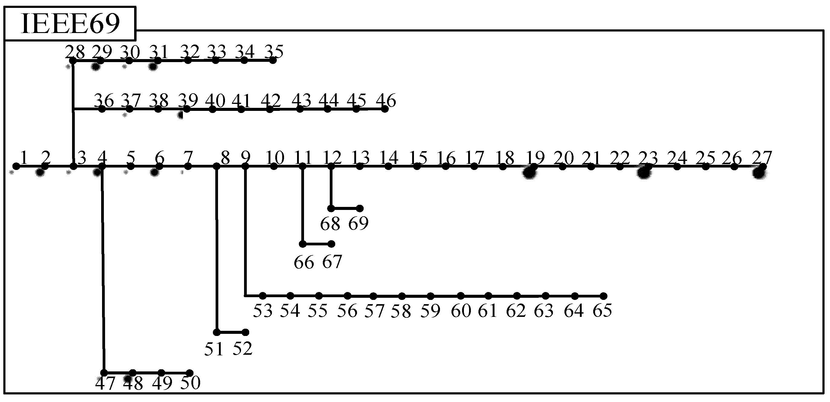
| IEEE69 | 1.556 | 1.356 | 1.356 | >5 h | 27.396 | 20.509 |
| IEEE33 | Time (s) | Network Loss (MW) | Original Network Loss (MW) | Disconnected Switch |
|---|---|---|---|---|
| Single-period | 1.355014 | 0.0256 | 0.0368 | 7 (6–7), 9 (8–9), 14 (13–14), 32 (31–32), 37 (24–28) |
| Multi-period | 153.404963 | 1.7080 | 2.4964 |
Disclaimer/Publisher’s Note: The statements, opinions and data contained in all publications are solely those of the individual author(s) and contributor(s) and not of MDPI and/or the editor(s). MDPI and/or the editor(s) disclaim responsibility for any injury to people or property resulting from any ideas, methods, instructions or products referred to in the content. |
© 2023 by the authors. Licensee MDPI, Basel, Switzerland. This article is an open access article distributed under the terms and conditions of the Creative Commons Attribution (CC BY) license (https://creativecommons.org/licenses/by/4.0/).
Share and Cite
Meng, W.; Song, D.; Deng, X.; Dong, M.; Yang, J.; Rizk-Allah, R.M.; Snášel, V. Dynamic Optimal Power Flow of Active Distribution Network Based on LSOCR and Its Application Scenarios. Electronics 2023, 12, 1530. https://doi.org/10.3390/electronics12071530
Meng W, Song D, Deng X, Dong M, Yang J, Rizk-Allah RM, Snášel V. Dynamic Optimal Power Flow of Active Distribution Network Based on LSOCR and Its Application Scenarios. Electronics. 2023; 12(7):1530. https://doi.org/10.3390/electronics12071530
Chicago/Turabian StyleMeng, Weiqi, Dongran Song, Xiaofei Deng, Mi Dong, Jian Yang, Rizk M. Rizk-Allah, and Václav Snášel. 2023. "Dynamic Optimal Power Flow of Active Distribution Network Based on LSOCR and Its Application Scenarios" Electronics 12, no. 7: 1530. https://doi.org/10.3390/electronics12071530
APA StyleMeng, W., Song, D., Deng, X., Dong, M., Yang, J., Rizk-Allah, R. M., & Snášel, V. (2023). Dynamic Optimal Power Flow of Active Distribution Network Based on LSOCR and Its Application Scenarios. Electronics, 12(7), 1530. https://doi.org/10.3390/electronics12071530