
A Novel Denoising Algorithm Based on Wavelet and Non-Local Moment Mean Filtering

Abstract
1. Introduction
2. Related Work

| Classification | Year | Author | Methods |
|---|---|---|---|
| Traditional image denoising methods | 2003 | Chen et al. [3] | Mathematics morphology |
| 2005 | Guan et al. [4] | Mean and median filtering approaches | |
| 2007 | Hu et al. [5] | Mean filtering, median filtering, and wavelet transform | |
| 2011 | Zhao et al. [6] | Improved median filtering | |
| 2018 | Yin et al. [7] | Improved wavelet threshold | |
| 2017 | Zhang et al. [8] | Threshold with wavelet transform | |
| 2022 | Wang et al. [9] | Wavelet transform combined with improved PSO | |
| 2022 | Kazuaki et al. [10] | Total variation regularization | |
| 2022 | Guo et al. [11] | Adaptive threshold and optimized weighted median filter | |
| 2021 | Yuan et al. [12] | Edge-Preserving Median Filter and Weighted Coding with Sparse Nonlocal Regularization | |
| 1990 | Perona et al. [13] | Anisotropic diffusion | |
| 1998 | Tomasi [14] | Bilateral filtering | |
| 2005 | Aharon et al. [15] | K-SVD | |
| 2007 | Kostadin et al. [16] | Sparse 3-D transform-domain collaborative filtering | |
| Deep learning approaches | 2021 | Wang et al. [17] | Attention neural network |
| 2021 | Ahmed et al. [18] | Stacked convolutional autoencoder | |
| 2021 | Huang et al. [19] | Unsupervised pseudo-siamese network | |
| 2021 | Wang et al. [20] | Convolutional neural network | |
| 2021 | Usui et al. [21] | Convolutional neural network | |
| 2022 | Rajesh et al. [22] | An evolutionary block-based network |
3. Methodology
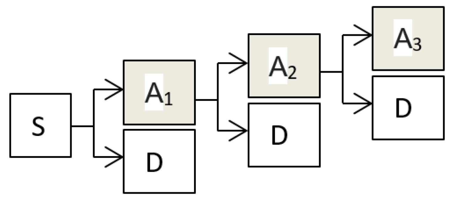
3.1. Multi-Scale Decomposition Denoising
3.2. Non-Local Moment Mean Filtering
| Algorithm 1: W-NMM filtering |
| Input: image I to be filtered t: radio of search window f: radio of similarity window h: degree of filtering 1. Take sym8 as the wavelet basis function to decompose the image in two layers. 2. Calculate the soft threshold according to Equation (6) on the high-frequency domains. 3. Denoise image I according to Equation (5) and obtained I’. 4. Symmetric padding I’; 5. For each pixel in I’(i,j) (i = f:M − f, j = f:N − f): i1 i + f; j1 j + f; Create objective window: W1= I’(i1 − f:i1 + f, j1 − f:j1 + f); 6. Set the borders of the neighboring window: rminmax(i1 − t, f + 1); rmaxmin(i1 + t, m + f); sminmax(j1 − t, f + 1); smaxmin(j1 + t, n + f); 7. For each pixel in W2(r,s): Set neighboring window: W2 = input2(r − f:r + f, s − f:s + f); 8. Calculate the moments of W1 and W2: n1 = hu_moments(W1); n2 = hu_moments(W2); 9. Calculate the similarity of W1 and W2 according to n1 and n2. 10. Calculate the Gaussian weight: wexp − d/h); 11. Find the maximum of w: wmax. sweightsweight + w; averageaverage + w × I’(r,s); end 12. Calculate the accumulation of average = average + wmax × I’(i,j); sweight = sweight + wmax; 13. Calculate denoised image Iout: if sweight > 0 Iout’(i,j) = average/sweight; else Iout’(i,j) = I’(i,j); end 14. end 15. Extract the image Iout with the size same to I from Iout’. |
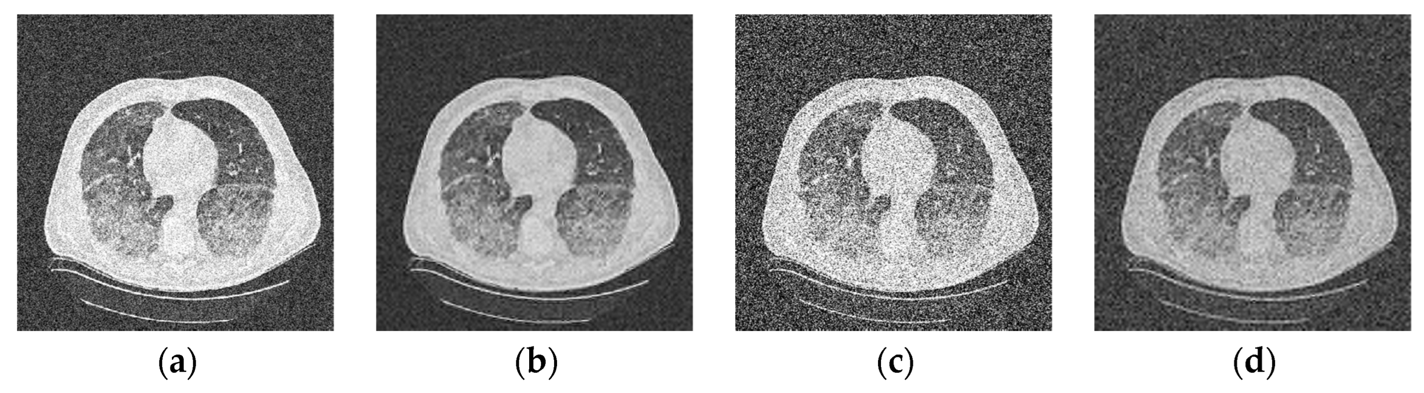
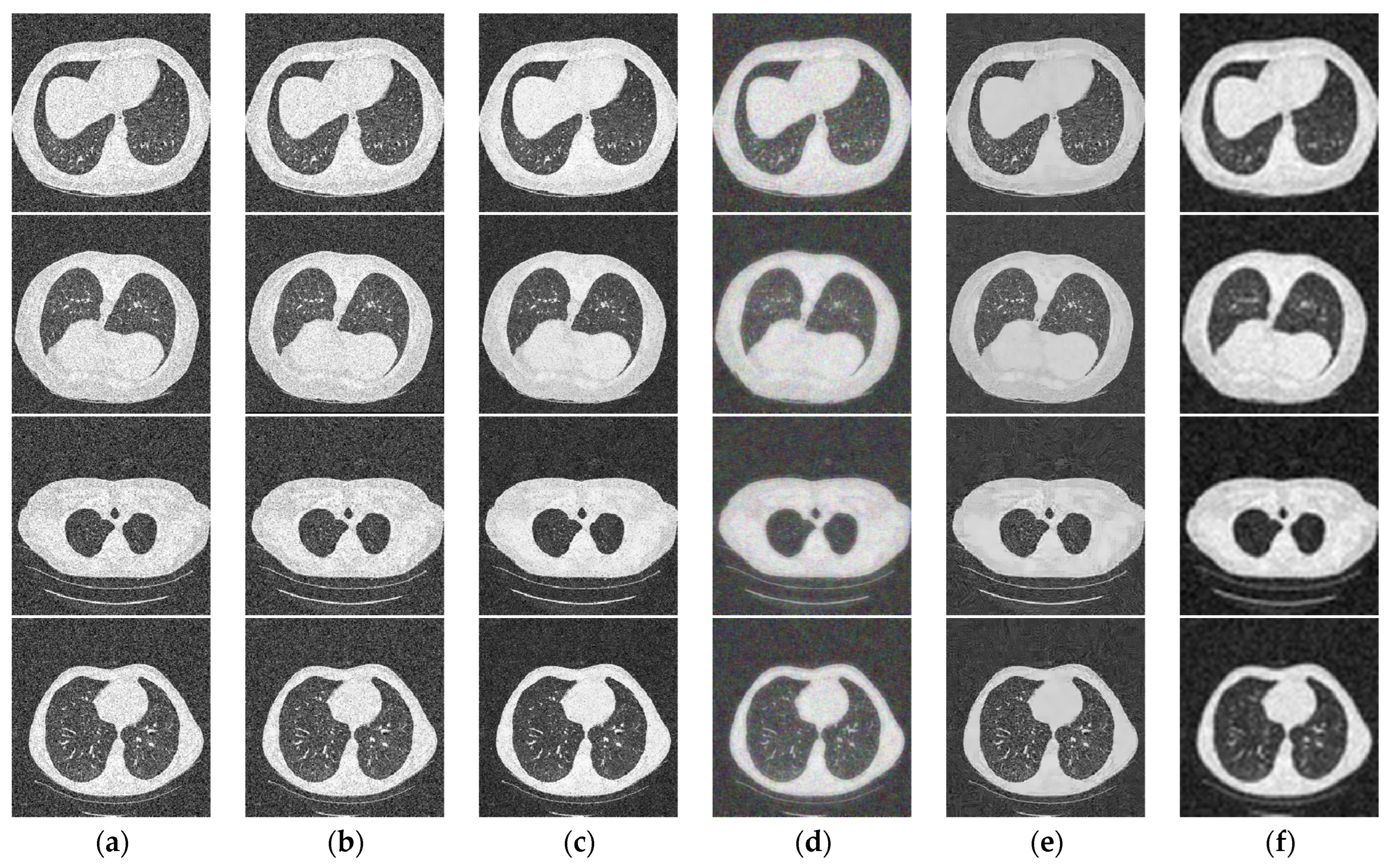
4. Experiment
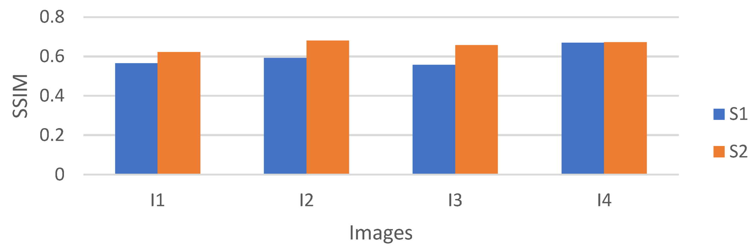
5. Discussion
6. Conclusions
Author Contributions
Funding
Data Availability Statement
Conflicts of Interest
Appendix A
| Abbreviations | Nomenclature |
|---|---|
| W | Wavelet |
| NLM | Non-local mean filter |
| NMM | Non-local moment mean filter |
| AD | Anisotropic diffusion filter |
| BF | Bilateral filter |
| BM3D | Block matching and 3D collaborative filtering |
| KSVD | Kernel singular value decomposition |
| PSNR | Peak signal to noise ratio |
| SSIM | Structural similarity index |
References
- Xu, M.; Xie, X. An efficient feature-preserving PDE algorithm for image denoising based on a spatial-fractional anisotropic diffusion equation. East Asian J. Appl. Math. 2021, 11, 788–807. [Google Scholar]
- Vaiyapuri, T.; Alaskar, H.; Sbai, Z.; Devi, S. GA-based multi-objective optimization technique for medical image denoising in wavelet domain. J. Intell. Fuzzy Syst. 2021, 41, 1575–1588. [Google Scholar] [CrossRef]
- Chen, H.; Zhou, C.H.; Wang, S.Z. Research based on mathematics morphology image chirp method. J. Eng. Graph. 2003, 2, 116–119. [Google Scholar]
- Guan, X.P.; Zhao, L.X.; Tang, Y.G. Mixed filter for image denoising. J. Image Graph. 2005, 10, 332–337. [Google Scholar]
- Hu, L.; Zhang, W.; Tan, Y.Q. Application and analysis about some arithmetics for image denoising. Inf. Technol. 2007, 7, 81–83. [Google Scholar]
- Zhao, G.C.; Zhang, L.; Wu, F.B. Application of improved median filtering algorithm to image de-noising. J. Appl. Opt. 2011, 32, 678–682. [Google Scholar]
- Yin, Q.S.; Dai, S.G. Research on image denoising algorithm based on improved wavelet threshold. Softw. Guide 2018, 17, 89–91. [Google Scholar]
- Zhang, X.; Turghunjan, A.T. Improvement of threshold image denoising algorithm with wavelet transform. Comput. Technol. Dev. 2017, 27, 81–84. [Google Scholar]
- Wang, G.; Guo, S.; Han, L.; Cekderi, A.B.; Song, X.; Zhao, Z. Asymptomatic COVID-19 CT image denoising method based on wavelet transform combined with improved PSO. Biomed. Signal Process. Control 2022, 76, 103707. [Google Scholar] [CrossRef]
- Kawahara, K.; Ishikawa, R.; Sasano, S.; Shibata, N.; Ikuhara, Y. Atomic-resolution STEM image denoising by total variation regularization. Microscopy 2022, 5, 302–310. [Google Scholar] [CrossRef]
- Guo, S.; Wang, G.; Han, L.; Song, X.; Yang, W. COVID-19 CT image denoising algorithm based on adaptive threshold and optimized weighted median filter. Biomed. Signal Process. Control 2022, 75, 103552. [Google Scholar] [CrossRef] [PubMed]
- Yuan, Q.; Peng, Z.; Chen, Z.; Guo, Y.; Yang, B.; Zeng, X. Edge-Preserving Median Filter and Weighted Coding with Sparse Nonlocal Regularization for Low-Dose CT Image Denoising Algorithm. J. Healthc. Eng. 2021, 2021, 6095676. [Google Scholar] [CrossRef] [PubMed]
- Perona, P.; Malik, J. Scale-space and edge detection using anisotropic diffusion. IEEE Trans. Pattern Anal. Mach. Intell. 1990, 12, 629–639. [Google Scholar] [CrossRef]
- Tomasi, C.; Manduchi, R. Bilateral filtering for gray and color images. In Proceedings of the International Conference on Computer Vision, Copenhagen, Denmark, 28–31 May 2002. [Google Scholar]
- Aharon, M.; Elad, M.; Bruckstein, A. K-SVD: Design of dictionaries for sparse representation. IEEE Trans. Signal Process. 2006, 54, 4311–4322. [Google Scholar] [CrossRef]
- Dabov, K.; Foi, A.; Katkovnik, V.; Egiazarian, K. Image denoising by sparse 3-D transform-domain collaborative filtering. IEEE Trans. Image Process. 2007, 16, 2080–2095. [Google Scholar] [CrossRef] [PubMed]
- Wang, Y.; Song, X.; Gong, G.; Li, N. A Multi-Scale Feature Extraction-Based Normalized Attention Neural Network for Image Denoising. Electronics 2021, 10, 319. [Google Scholar] [CrossRef]
- Ahmed, A.S.; El-Behaidy, W.H.; Youssif, A.A. Medical image denoising system based on stacked convolutional autoencoder for enhancing 2-dimensional gel electrophoresis noise reduction. Biomed. Signal Process. Control 2021, 69, 102842. [Google Scholar] [CrossRef]
- Huang, C.; Hong, D.; Yang, C.; Cai, C.; Tao, S.; Clawson, K.; Peng, Y. A new unsupervised pseudo-siamese network with two filling strategies for image denoising and quality enhancement. Neural Comput. Appl. 2021, 1, 1–9. [Google Scholar] [CrossRef]
- Wang, J.; Tang, Y.; Zhang, J.; Yue, M.; Feng, X. Convolutional neural network-based image denoising for synchronous measurement of temperature and deformation at elevated temperature. Optik 2021, 241, 166977. [Google Scholar] [CrossRef]
- Usui, K.; Ogawa, K.; Goto, M.; Sakano, Y.; Kyougoku, S.; Daida, H. Quantitative evaluation of deep convolutional neural network-based image denoising for low-dose computed tomography. Vis. Comput. Ind. Biomed. Art 2021, 4, 21. [Google Scholar] [CrossRef]
- Rajesh, C.; Kumar, S. An evolutionary block based network for medical image denoising using Differential Evolution. Appl. Soft Comput. 2022, 121, 108776. [Google Scholar] [CrossRef]
- Gao, Q.W.; Li, B.; Xie, G.J.; Zhuang, Z.Q. An image de-noising method based on stationary wavelet transform. J. Comput. Res. Dev. 2002, 39, 1689–1694. [Google Scholar]
- Donoho, D.L.; Johnstone, J.M. Ideal spatial adaptation by wavelet shrinkage. Biometrika 1994, 81, 425–455. [Google Scholar] [CrossRef]
- Buades, A.; Coll, B.; Morel, J.M. A non-local algorithm for image denoising. In Proceedings of the 2005 IEEE Computer Society Conference on Computer Vision and Pattern Recognition (CVPR’05), San Diego, CA, USA, 20–26 June 2005. [Google Scholar]
- Yi, Z.L.; Yin, D.; Hu, A.Z.; Zhang, R. SAR Image Despeckling Based on Non-local Means Filter. J. Electron. Inf. Technol. 2012, 34, 950–953. [Google Scholar]
- Hu, M.-K. Visual pattern recognition by moment invariants. IEEE Trans. Inf. Theory 1962, 8, 179–187. [Google Scholar] [CrossRef]
- Huynh-Thu, Q.; Ghanbari, M. Scope of validity of PSNR in image/video quality assessment. Electron. Lett. 2008, 44, 800–801. [Google Scholar] [CrossRef]
- Wang, Z.; Bovik, A.C.; Sheikh, H.R.; Simoncelli, E.P. Image Quality Assessment: From Error Visibility to Structural Similarity. IEEE Trans. Image Process. 2004, 13, 600–612. [Google Scholar] [CrossRef]
- Depeursinge, A.; Vargas, A.; Platon, A.; Geissbuhler, A.; Poletti, P.-A.; Müller, H. Building a reference multimedia database for interstitial lung diseases. Comput. Med. Imaging Graph. 2012, 36, 227–238. [Google Scholar] [CrossRef]


| Image | I1 | I2 | I3 | I4 | ||||
|---|---|---|---|---|---|---|---|---|
| Metrics | PSNR | SSIM | PSNR | SSIM | PSNR | SSIM | PSNR | SSIM |
| AD | 18.48 | 0.2964 | 18.38 | 0.2407 | 18.42 | 0.2352 | 18.27 | 0.3298 |
| BF | 20.37 | 0.3593 | 19.95 | 0.3004 | 20.21 | 0.2965 | 19.71 | 0.3731 |
| KSVD | 22.61 | 0.5578 | 22.49 | 0.3787 | 23.34 | 0.5512 | 22.67 | 0.5660 |
| BM3D | 20.66 | 0.5479 | 23.63 | 0.5736 | 22.80 | 0.4603 | 21.15 | 0.4830 |
| W-NMM | 22.67 | 0.6219 | 24.20 | 0.6798 | 23.62 | 0.6557 | 22.43 | 0.6714 |
Disclaimer/Publisher’s Note: The statements, opinions and data contained in all publications are solely those of the individual author(s) and contributor(s) and not of MDPI and/or the editor(s). MDPI and/or the editor(s) disclaim responsibility for any injury to people or property resulting from any ideas, methods, instructions or products referred to in the content. |
© 2023 by the authors. Licensee MDPI, Basel, Switzerland. This article is an open access article distributed under the terms and conditions of the Creative Commons Attribution (CC BY) license (https://creativecommons.org/licenses/by/4.0/).
Share and Cite
Liu, C.; Zhang, L. A Novel Denoising Algorithm Based on Wavelet and Non-Local Moment Mean Filtering. Electronics 2023, 12, 1461. https://doi.org/10.3390/electronics12061461
Liu C, Zhang L. A Novel Denoising Algorithm Based on Wavelet and Non-Local Moment Mean Filtering. Electronics. 2023; 12(6):1461. https://doi.org/10.3390/electronics12061461
Chicago/Turabian StyleLiu, Caixia, and Li Zhang. 2023. "A Novel Denoising Algorithm Based on Wavelet and Non-Local Moment Mean Filtering" Electronics 12, no. 6: 1461. https://doi.org/10.3390/electronics12061461
APA StyleLiu, C., & Zhang, L. (2023). A Novel Denoising Algorithm Based on Wavelet and Non-Local Moment Mean Filtering. Electronics, 12(6), 1461. https://doi.org/10.3390/electronics12061461