Dual-Filter Architecture for Blind Feedback Recovery of the Symbol Timing in Bandlimited Optical Intensity Channels

Abstract

Reliable recovery of transmission parameters is of paramount importance not only for radio frequency receivers, but also for optical wireless communication solutions. This paper discusses a feedback algorithm for recovering the symbol timing in the context of a bandlimited optical intensity link. The link is determined by a PAM scheme and pulse shaping with squared raised cosine or double jump functions. When preambles or pilot sequences are not available to the receiver, non-data-aided (blind) recovery concepts are useful for tracking smaller variations of the timing error affecting the payload data. The current state-of-the-art solution uses a Gardner detector with two samples per symbol, although this introduces a non-negligible amount of inter-symbol interference resulting in an error floor. To avoid this drawback, the authors propose a dual-filter approach which includes an appropriately designed filter operated in parallel to the receiver filter. Despite the additional complexity of the dual-filter architecture, the recovery loop is very simple and requires only one sample per symbol, representing the lowest degree of complexity in this respect. Open-loop characteristic, jitter performance, and acquisition behavior of the suggested recovery loop are investigated.

1. Introduction

Comparing radio frequency (RF) to optical wireless communication (OWC) techniques, the benefits of the latter are well known: no regulatory and license issues, rather inexpensive and easy to deploy, extremely high throughput, and no problems with data security, just to mention the most significant aspects in this context [1,2,3,4]. A nice overview in this respect is also given by the authors in [5,6], both from a historical as well as a technical point of view. Moreover, unlimited bandwidth is frequently mentioned as an important feature, but this is not true in the strict sense due to inevitable hardware constraints of opto-electronic components in transmitter and receiver units [7]. A strong argument for a bandlimited approach is also that powerful algorithms for parameter estimation and synchronization normally used in RF receivers [8,9] would become applicable to OWC systems as well. Further reasons, beyond OWC, for bandwidth constraints are related to multipath distortions in diffuse optical indoor systems or dispersion effects in optical fiber networks [10,11].

Focusing in the following on intensity modulation, it is to be noticed that the optical domain tolerates no negative signal components. For a bandlimited approach with pulse shapes used for RF solutions, this is simply achieved by a suitably selected bias or offset signal, with respect to a subcarrier system discussed in [12,13,14,15] or via an M-ary PAM scheme investigated in [10,11]. However, such concepts are not very efficient in terms of power and energy in case that no harvesting is implemented. Therefore, a unipolar pulse design satisfying the Nyquist criterion has been suggested in [7]. It could be demonstrated by the author that the squared impulse response derived from a raised cosine function defined in the frequency domain, simply denoted as the squared raised cosine (SRC) method, fulfills this requirement.

Unfortunately, there exists no simple real-valued root-Nyquist solution for SRC shapes satisfying the non-negativity constraint, although this would be necessary to maximize the signal-to-noise ratio (SNR) at the output of a receiver-matched filter. Instead, a rectangular filter performing a flat behavior in the frequency domain of interest is frequently implemented in practice. An alternative would be the approach introduced in [16] to obtain a non-negative impulse response, but this results in an unconstrained min-max optimization procedure, which has to be solved by numerical means whenever a new design is required.

Not only for RF but also for OWC solutions, the most important transmission parameters must be successfully recovered by powerful algorithms [8,9]. Otherwise, subsequent receiver stages, such as symbol detection and error correction units, cannot be operated reliably. Certainly, in case of optical intensity links, carrier frequency and phase need not be considered, whereas estimation and synchronization of symbol timing and clocking is of paramount importance. Screening the open literature in this context, not much material is available. To the best of the authors’ knowledge, it is the first time that this problem has been addressed for SRC shapes in [17]. Under the assumption that the user data are known to the receiver unit in the form of preambles or pilot sequences, a data-aided (DA) feedforward algorithm could be derived from the maximum likelihood principle and compared to the modified Cramer-Rao lower bound (MCRLB) as the major figure of merit, when it comes to the estimation of a transmission parameter, in general [18].

The work in [17] has been extended in [19,20] by a non-data-aided (NDA) feedforward (FF) as well as a feedback (FB) architecture that do not need any knowledge about data such that payload symbols must be used for this purpose. Specifically, the FB synchronizer in [20] is realized with a single receiver filter and a Gardner detector (TED), which necessitates two samples per symbol period. Nevertheless, this moderate form of oversampling causes a jitter variance ending up in an error floor at higher SNR values. This drawback is avoided by the approach introduced in the current contribution, where a second filter is operated in parallel to the receiver filter so that no oversampling is required for the recovery loop.

The remainder of the paper is organized as follows: Section 2 focuses on the signal and channel model used for analytical and simulation work. In Section 3, the dual-filter solution is developed. This is discussed in Section 4 and Section 5 in terms of open-loop characteristics, jitter performance, and acquisition behavior. Finally, conclusions are drawn in Section 6.

2. Signal and Channel Model

Since the current paper is a follow-up activity of the results achieved in [17] and [19,20], the applicable signal and channel model is essentially the same. From this point of view, it makes sense to recapitulate this model for clarity and readability reasons. This gives us also the chance to introduce some basic notations used throughout the paper.

First, it is assumed that the real-valued data symbols a_k, $k\in \mathbb{Z}$, are independent and identically distributed (i.i.d.) elements of an M-ary PAM alphabet $\mathcal{A}$. For convenience, the alphabet is organized such that the symbols are normalized to unit energy, i.e., ${\eta }_a=\mathbb{E}[a_k^2]=1$, where $\mathbb{E}[\cdot ]$ denotes the expectation operator. With ${\eta }_M=\frac{1}{6}(M-1)(2M-1)$ the PAM symbols are now given as $a_k\in \mathcal{A}=\frac{1}{\sqrt{{\eta }_M}}\{\hspace{0.17em}0,\hspace{0.17em}\hspace{0.17em}1,\hspace{0.17em}\hspace{0.17em}\dots ,\hspace{0.17em}\hspace{0.17em}M-1\hspace{0.17em}\}$. This means that the average value is determined by

$${\mu }_a=\mathbb{E}[a_k]=\frac{1}{\sqrt{{\eta }_M}}\hspace{0.17em}\hspace{0.17em}\frac{M-1}{2}=\sqrt{\frac{3\hspace{0.17em}(M-1)}{2\hspace{0.17em}(2M-1)}}$$

(1)

Furthermore, it is assumed that the pulses in the transmitter station are either shaped by a squared raised cosine (SRC) or a squared double jump (SDJ) function [7] expressed as

$$h(t)=\frac{1}{\sqrt{T}}\hspace{0.17em}\hspace{0.17em}\{\begin{array}{l}\hspace{0.17em}{\left(\sin \mathrm{c}(t/T)\hspace{0.17em}\hspace{0.17em}\frac{\cos (\pi \hspace{0.17em}\alpha t/T)}{1-{(2\alpha t/T)}^2}\right)}^2\hspace{0.17em}\hspace{0.17em}\hspace{0.17em}\hspace{0.17em}\hspace{0.17em}\hspace{0.17em}\dots \hspace{0.17em}\hspace{0.17em}\hspace{0.17em}\mathrm{SRC}\\ \hspace{0.17em}{\left(\frac{1-\alpha }{2}\sin \mathrm{c}[(1-\alpha )t/T]\hspace{0.17em}\hspace{0.17em}+\frac{1+\alpha }{2}\sin \mathrm{c}[(1+\alpha )t/T]\right)}^2\hspace{0.17em}\hspace{0.17em}\hspace{0.17em}\hspace{0.17em}\hspace{0.17em}\hspace{0.17em}\dots \hspace{0.17em}\hspace{0.17em}\hspace{0.17em}\mathrm{SDJ}\end{array}$$

(2)

where $\mathrm{sinc}(x)=\sin (\pi x)/(\pi x)$, 0 ≤ α ≤ 1 is the excess bandwidth (roll-off factor), and T stands for the symbol period the OWC link is operated which. Note that SRC and SDJ shapes satisfy both the non-negativity and the Nyquist criterion, exemplified in Figure 1 for α ∈ {0.0, 0.5, 1.0}.

It has been proved in [7] that SDJ pulses are optimal insofar as the average optical power achieves a minimum for a given value of α, which is a major motivation to compare this kind of pulses to SRC shapes. Note also that SRC and SDJ are equivalent for α = 0, which represents the minimum bandwidth (MBW) case with $h(t)=\frac{1}{\sqrt{T}}{\mathrm{sinc}}^2(t/T)$, whereas for α = 1, with $h(t)=\frac{1}{\sqrt{T}}{\left(\frac{\mathrm{sinc}(2t/T)}{1-{(2t/T)}^2}\right)}^2$ for SRC and $h(t)=\frac{1}{\sqrt{T}}{\mathrm{sinc}}^2(2t/T)$ for SDJ, the required bandwidth achieves a maximum. By detailed inspection of Figure 1, it can also be observed that the width of the main lobe shrinks when α increases and that this effect is more pronounced for SDJ.

However, irrespective of the pulse shape finally selected, the generated transmitter signal can be generically written as

$$s(t)=\hspace{0.17em}{\displaystyle \sum _k{a}_{k\hspace{0.17em}}h(t-kT)}$$

(3)

It is clear that the observation window for the estimation procedure is usually much smaller than the coherence time of a fading process the channel might suffer from, i.e., the channel state does not change significantly over this period of time, so that fading effects need not be taken into account. Related to this observation interval, this means also that the optical signal at the receiver side is only affected by some propagation loss and a delay in time, henceforth denoted by K_l and τ, respectively. Then, by introduction of the electro-optical conversion factor K₀ and the detector responsivity R_d in the transmitter and receiver units, we have a gain factor $A=R_{d\hspace{0.17em}}{K}_{l\hspace{0.17em}}{K}_0$ characterizing the OWC link. Assuming also that the signal part $x(t)=A\cdot s(t-\tau )$ is distorted by zero-mean white Gaussian noise w(t) with variance ${\sigma }_w^2$, the receiver signal can be expressed as

$$r(t)=x(t)+\hspace{0.17em}w(t)=A\cdot s(t-\tau )+\hspace{0.17em}w(t)$$

(4)

Certainly, before being treated in further stages of operation, the signal in (4) has to pass the receiver filter q(t), whose output z(t) is appropriately sampled to avoid alias effects. For convenience, the signal and channel model used for analytical and simulation work is summarized in Figure 2.

In addition, the average optical power is defined as $P_0={\mu }_{a\hspace{0.17em}}\overline{h}$, where

$$\overline{h}=\frac{1}{\sqrt{T}}{\displaystyle \underset{-\infty }{\overset{\infty }{\int }}h(t)\hspace{0.17em}dt}=\{\begin{array}{l}1-\frac{\alpha }{4}\hspace{0.17em}\hspace{0.17em}\hspace{0.17em}\hspace{0.17em}\hspace{0.17em}\dots \hspace{0.17em}\hspace{0.17em}\hspace{0.17em}\mathrm{SRC}\\ 1-\frac{\alpha }{2}\hspace{0.17em}\hspace{0.17em}\hspace{0.17em}\hspace{0.17em}\hspace{0.17em}\dots \hspace{0.17em}\hspace{0.17em}\hspace{0.17em}\mathrm{SDJ}\end{array}$$

(5)

and the average electrical SNR at the receiver is introduced as

$${\gamma }_s=\frac{A^2{P}_0^2}{{\sigma }_w^2}$$

(6)

3. Dual-Filter Architecture

Regarding the maximum likelihood algorithm developed for symbol timing estimation in [17], it could be verified that the receiver filter with impulse response q(t) must be proportional to the signal shape given by (2). However, this violates the Nyquist criterion guaranteeing a rather simple detection of symbols. As an alternative, it is frequently suggested to employ a direct-sampling receiver. Specifically, this means that q(t) exhibits a flat behavior in the frequency domain occupying the same bandwidth as the user signal in (3), i.e., $Q(f)=ℱ[q(t)]=\sqrt{T}$ for $\left|f\right|\hspace{0.17em}\hspace{0.17em}\le (1+\alpha )/T$ and zero elsewhere. Applying the rules for Fourier transforms [21] simply yields

$$q(t)={ℱ}^{-1}[Q(f)]=\hspace{0.17em}\frac{2(1+\alpha )}{\sqrt{T}}\sin \mathrm{c}[2(1+\alpha )t/T]$$

(7)

The output of the filter is then determined by

$$z(t)=r(t)\otimes q(t)=x(t)+n(t)$$

(8)

with ⊗ as the convolutional operator. Hence, the signal component is furnished as

$$x(t)=A{\displaystyle \sum _i{a}_{i\hspace{0.17em}}g(t-iT-\tau )}$$

(9)

where $g(t)=h(t)\otimes q(t)=\sqrt{T}h(t)$ and $n(t)=w(t)\otimes q(t)$ is the corresponding noise component. Some remarks are most helpful in this respect:

• g(t) is proportional to h(t), which means that the Nyquist criterion is satisfied.
• For SRC and SDJ shapes given by (2), the Fourier transform $G(f)=ℱ[g(t)]$ is strictly bandlimited by $\pm (1+\alpha )/T$.
• n(t) is a zero-mean non-white Gaussian process.

As already mentioned in the introductory section, it is desirable to explore a FB structure for symbol timing recovery, which employs a second filter with impulse response $\dot{q}(t)$ operated in parallel to q(t), as shown in Figure 3.

In the context of RF systems using a square-root raised cosine (SRRC) filter for pulse shaping, it has been demonstrated in [22] that a data-blind symbol synchronizer can be realized with a couple of benefits if this parallel filter is designed by considering the extended zero-crossing property. Applying this concept also to our optical link introduced previously, this would mean that $\dot{g}(t)=h(t)\otimes \dot{q}(t)$ must vanish at all integer multiples of T, i.e., $\dot{g}(kT)=0,\hspace{0.17em}\hspace{0.17em}\hspace{0.17em}k\in \mathbb{Z}$. This goal is easily achieved with the first-order derivative of q(t) so that $\dot{Q}(f)=ℱ[\dot{q}(t)]=j2\pi fT\hspace{0.17em}Q(f)$. As a consequence, the corresponding impulse response is obtained as

$$\dot{q}(t)={ℱ}^{-1}[\dot{Q}(f)]=\frac{1}{\pi \sqrt{T}}\left\{\frac{2\pi (1+\alpha )\cos [2\pi (1+\alpha )t/T]}{t/T}-\frac{\sin [2\pi (1+\alpha )t/T]}{{(t/T)}^2}\right\}$$

(10)

Consequently, the output of the parallel filter is given by

$$\dot{z}(t)=r(t)\otimes \dot{q}(t)=\dot{x}(t)+\dot{n}(t)$$

(11)

with the signal part specified as

$$\dot{x}(t)=A{\displaystyle \sum _i{a}_{i\hspace{0.17em}}\dot{g}(t-iT-\tau )}$$

(12)

and the noise part determined by $\dot{n}(t)=w(t)\otimes \dot{q}(t)$. Similar to the noise component n(t) in (8), $\dot{n}(t)$ is a zero-mean non-white Gaussian process. Furthermore, it is to be noticed that $\mathbb{E}[\dot{n}(t)\hspace{0.17em}n(t)]=0$, which is due to the orthogonal characteristics of q(t) and $\dot{q}(t)$. Finally, it is clear that the Fourier transform of $\dot{g}(t)$ is furnished by $\dot{G}(f)=ℱ[\dot{g}(t)]=j2\pi fT\hspace{0.17em}G(f)$.

By detailed inspection of Figure 3, it can be observed that the filter outputs, sampled at integer multiples of the symbol period, i.e., $z_k=z(kT)$ and ${\dot{z}}_k=\dot{z}(kT)$, are processed in the timing error detector (TED). According to the approach in [22], it is proposed that the error signal is simply computed as

$$e_k={\dot{z}}_k{z}_k$$

(13)

This error signal is then fed to the loop filter determined by its z-transform F_e(z). Since it is assumed that the fluctuations of the timing offset τ are much slower than the settling period of the FB loop, a first-order structure is sufficient to follow these variations so that the loop filter reduces to a pure constant. The integrator–mandatory for an analog implementation—is in the digital domain replaced by a running sum, which controls the sampling process, as depicted in Figure 3. It is to be observed that the recovery loop requires no oversampling, i.e., only the absolute minimum of one sample per symbol period is needed to operate the structure in Figure 3.

4. Open-Loop Characteristic

The open-loop characteristic or S-curve is a major figure of merit when it comes to the recovery of a transmission parameter by means of a tracking loop. Given that the loop is open, the S-curve is defined as the average output of the corresponding detector module [8]. Related to the timing synchronizer shown in Figure 3, this can be generically expressed as

$$S(\tau )=\mathbb{E}[e_k|{\widehat{\tau }}_k=0]$$

(14)

Recalling that $z_k=\hspace{0.17em}{x}_k+\hspace{0.17em}{n}_k$ and ${\dot{z}}_k=\hspace{0.17em}{\dot{x}}_k+\hspace{0.17em}{\dot{n}}_k$, (13) is substituted into (14), which yields

$$S(\tau )=\mathbb{E}[{\dot{z}}_k{z}_k]=\mathbb{E}[{\dot{x}}_k{x}_k]$$

(15)

after having taken into account that the noise samples $n_k$ and ${\dot{n}}_k$ are zero-mean Gaussian and orthogonal, i.e., $\mathbb{E}[n_k]=\mathbb{E}[{\dot{n}}_k]=\mathbb{E}[n_k{\dot{n}}_k]=0$. Furthermore, by introduction of the normalized timing error $\epsilon =\tau /T$, the signal samples are given by

$$x_k=x(kT)=A{\displaystyle \sum _i{a}_{i\hspace{0.17em}}g[(k-i-\epsilon )T]}$$

(16)

and

$${\dot{x}}_k=\dot{x}(kT)=A{\displaystyle \sum _i{a}_{i\hspace{0.17em}}\dot{g}[(k-i-\epsilon )T]}$$

(17)

Plugging in the next steps (16) and (17) into (15), one obtains for the i.i.d. symbols $a_i\in \mathcal{A}$ after a re-arrangement of indexes,

$$\begin{array}{ll}\mathbb{E}[{\dot{x}}_k{x}_k]& =\mathbb{E}\left[A^2{\displaystyle \sum _i{\displaystyle \sum _l{a}_{i\hspace{0.17em}}{a}_{l\hspace{0.17em}}\dot{g}[(k-i-\epsilon )T]\hspace{0.17em}g[(k-l-\epsilon )T]}}\right]\\ & =A^2{\eta }_a{\displaystyle \sum _k\dot{g}[(k-\epsilon )T]\hspace{0.17em}g[(k-\epsilon )T]}\\ & +A^2{\mu }_a^2{\displaystyle \sum _k{\displaystyle \sum _{i\ne 0}\dot{g}[(k-\epsilon )T]\hspace{0.17em}g[(k-i-\epsilon )T]}}\hspace{0.17em}\hspace{0.17em}\end{array}$$

(18)

As shown in Appendix A, the infinite sums in (18) may be rewritten by means of the Fourier transforms for $g(t)$ and $\dot{g}(t)$. Since $G(f)=\sqrt{T}ℱ[h(t)]$ and $\dot{G}(f)=j2\pi fT\hspace{0.17em}G(f)$ are strictly bandlimited by $\pm (1+\alpha )/T$ for SRC and SDJ shapes, the first sum in (18) can be reformulated according to (A6):

$$\begin{array}{ll}{\mathsf{\Phi }}_0(\alpha ,\hspace{0.17em}\hspace{0.17em}\epsilon )& ={\displaystyle \sum _k\dot{g}[(k-\epsilon )T]\hspace{0.17em}g[(k-\epsilon )T]}\\ & =\frac{1}{T}{\displaystyle \underset{-(1+\alpha )/T}{\overset{(1+\alpha )/T}{\int }}\dot{G}(f){\displaystyle \sum _{m=-3}^{3}G\left(\frac{m}{T}-f\right)\hspace{0.17em}{e}^{-j2\pi m\hspace{0.17em}\epsilon }df}}\end{array}$$

(19)

Doing the same with the double sum in (18) yields

$$\begin{array}{ll}{\mathsf{\Phi }}_1(\alpha ,\hspace{0.17em}\hspace{0.17em}\epsilon )& ={\displaystyle \sum _k{\displaystyle \sum _{i\ne 0}\dot{g}[(k-\epsilon )T]\hspace{0.17em}g[(k-i-\epsilon )T]}}\\ & ={\displaystyle \sum _{i\ne 0}\hspace{0.17em}\frac{1}{T}{\displaystyle \underset{-(1+\alpha )/T}{\overset{(1+\alpha )/T}{\int }}\dot{G}(f)\hspace{0.17em}{e}^{j2\pi ifT}{\displaystyle \sum _{m=-3}^{3}G\left(\frac{m}{T}-f\right)\hspace{0.17em}{e}^{-j2\pi m\hspace{0.17em}\epsilon }df}}}\hspace{0.17em}\end{array}$$

(20)

Introducing now, for simplification reasons, the terms

$${\mathsf{\Psi }}_m(\alpha )={\psi }_{0,m}(\alpha )+2{\mu }_a^2{\displaystyle \sum _{i\ge 1}{\psi }_{i,m}(\alpha )}$$

(21)

and

$${\psi }_{i,m}(\alpha )=\frac{2\pi }{T}{\displaystyle \underset{-(1+\alpha )/T}{\overset{(1+\alpha )/T}{\int }}fT\hspace{0.17em}G(f)\hspace{0.17em}G\left(\frac{m}{T}-f\right)\hspace{0.17em}\cos (2\pi ifT)\hspace{0.17em}df}$$

(22)

the S-curve in (14) is, after some lengthy but straightforward algebra, most elegantly expressed as

$$S(\epsilon )=A^2[{\mathsf{\Phi }}_0(\alpha ,\hspace{0.17em}\hspace{0.17em}\epsilon )+{\mu }_a^2\hspace{0.17em}{\mathsf{\Phi }}_1(\alpha ,\hspace{0.17em}\hspace{0.17em}\epsilon )]=2A^2{\displaystyle \sum _{m=1}^3{\mathsf{\Psi }}_m(\alpha )\hspace{0.17em}\sin (2\pi m\epsilon )}$$

(23)

where it has already been taken into account that η_a = 1 and Ψ₀(α) = 0; the latter is easily explained by the fact that ψ_i,0(α) = 0 due to the even symmetry of G(f).

Apart from α = 0, the finite integral in (22) must be evaluated by numerical means. Luckily, G(f) is for SRC and SDJ shapes given in closed form; since this is a rather bulky relationship in piecewise form, it is not shown here for reasons of clarity and readability. Moreover, it could be verified that |ψ_i,m(α)| decreases monotonically with increasing indexes $i\in \mathbb{N}$, irrespective of the chosen values of m and α. Therefore, the summation in (21) will be executed until this term drops below a predefined threshold, such as 10⁻⁵, to achieve the necessary accuracy. In

Table 1. Coefficients for dual-filter solutions (4-PAM).

	SRC			SDJ
α	Ψ1(α)	Ψ2(α)	Ψ3(α)	Ψ1(α)	Ψ2(α)	Ψ3(α)
0.0	0.187	0.0	0.0	0.187	0.0	0.0
0.1	0.237	0.001	0.0	0.291	0.003	0.0
0.2	0.287	0.003	0.0	0.390	0.013	0.0
0.3	0.335	0.006	0.0	0.478	0.031	0.0
0.4	0.383	0.012	0.0	0.565	0.059	0.0
0.5	0.428	0.019	0.0	0.639	0.099	0.0
0.6	0.472	0.028	1.66 × 10−10	0.693	0.152	0.0
0.7	0.514	0.039	9.38 × 10−8	0.735	0.215	0.002
0.8	0.554	0.053	2.62 × 10−6	0.762	0.286	0.008
0.9	0.590	0.069	1.04 × 10−5	0.775	0.362	0.018
1.0	0.624	0.087	3.95 × 10−5	0.773	0.442	0.036

below, the numerical values of Ψ_m(α) have been computed for different values of α; although the table describes a 4-PAM scheme, the following observations are valid for other PAM constellations, as well:

• For α = 0, which indicates the MBW case, there is no overlap at all between G(f) and G(m/T − f), m = 2 and 3, so that Ψ₂(0) = Ψ₃(0) = 0; hence, the S-curve performs a pure sinusoidal shape determined by Ψ₁(0), which is available in closed form, as demonstrated in Appendix B;
• For 0 < α ≤ 0.5, Ψ₃(α) = 0, because G(f) and G(3/T − f) do not overlap;
• For SRC shapes, Ψ₂(α) and Ψ₃(α) are much smaller than Ψ₁(α) irrespective of α, which means that the S-curves approximate a sinusoidal function; this does not hold true for SDJ, where Ψ₂(α) is in the order of Ψ₁(α) for α > 0.5.

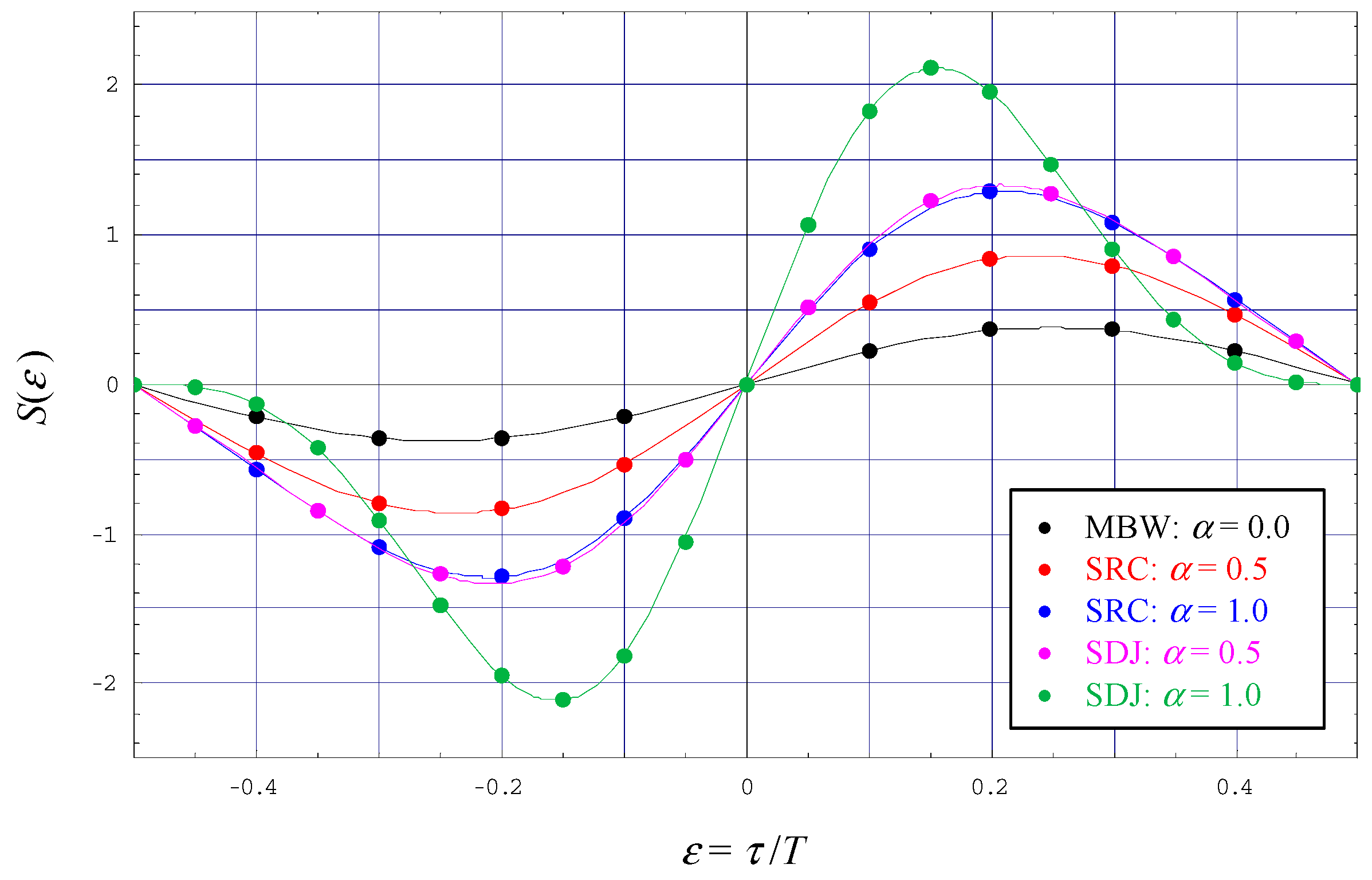
For 4-PAM signals, A = 1 and α ∈ {0.0, 0.5, 1.0}, the open-loop characteristic in (23) has been verified for SRC and SDJ scenarios by Monte Carlo simulations in Figure 4. The diagram confirms the observations drawn from Table 1: SRC shapes produce an S-curve that differs only slightly from a pure sinusoidal function at larger values of α, whereas for SDJ the corresponding S-curves begin to deviate.

By detailed inspection of (23), it is easily ascertained that S(0) = 0. This means that the TED module in Figure 3 exhibits no bias effect, which is of paramount importance for reliable recovery of the symbol timing. Furthermore, one can immediately compute the slope in the stable equilibrium point at ε = 0, which is needed for a linearized description of the tracking loop, as it is usually applied for small deviations from the equilibrium point. Regarding the S-curve in (23), this yields

$$K_e={\frac{\partial S(\epsilon )}{\partial \epsilon }\hspace{0.17em}|}_{\epsilon =0}=4A^2\pi {\displaystyle \sum _{m=1}^3\hspace{0.17em}m\hspace{0.17em}{\mathsf{\Psi }}_m(\alpha )}$$

(24)

For 4-PAM and 16-PAM schemes, Figure 5 shows the evolution of (24) as a function of the roll-off factor for SRC as well as SDJ pulses. It can be seen that the difference between 4-PAM and 16-PAM constellations is rather small. It can also be seen that K_e increases with increasing values of α, although this behavior is more pronounced for SDJ. Certainly, for α = 0 (MBW case), the slopes are the same for SRC and SDJ.

5. Jitter Performance and Acquisition Behavior

Apart from the open-loop characteristic discussed previously, the jitter performance is the second figure of merit regarding the synchronization of a transmission parameter. Recovering the symbol timing, it can be assumed that the fluctuation of $\epsilon =\tau /T$ is much slower than the settling period of the tracking loop. In this case, a first-order structure can be used, in which the loop filter boils down to a simple constant given by K_T. Focusing on the tracking mode with only small deviations from the stable equilibrium point, the jitter variance is determined by the one-sided noise bandwidth of the loop [8]; normalized by the symbol period, the latter is determined by

$$B_L{T}_e=\frac{{\mathsf{\Lambda }}_e}{2(2-{\mathsf{\Lambda }}_e)}$$

(25)

where ${\mathsf{\Lambda }}_e=K_T{K}_e$ denotes the loop gain for a first-order synchronizer. Conditioned on a given value of $B_L{T}_e$, this means that the slope $K_e$ of the S-curve in the stable equilibrium point must be known so that the filter constant $K_T$ can be computed; usually, ${\mathsf{\Lambda }}_e\ll 1$, which means that $B_L{T}_e\approx {\mathsf{\Lambda }}_e/4$.

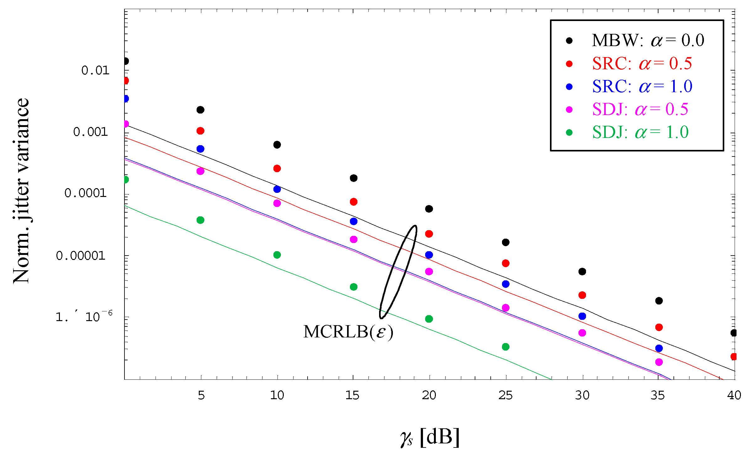
For a 4-PAM signal, $B_L{T}_e={10}^{-3}$, and different values of α, Figure 6 illustrates the evolution of the normalized jitter variance ${\sigma }_e^2=\mathbb{E}[{(\epsilon -\widehat{\epsilon })}^2]$ as a function of the average electrical SNR denoted by γ_s. For comparison purposes, the modified Cramer-Rao lower bound (MCRLB) is shown as well [23,24]. This represents the theoretical limit of the jitter variance, which has been derived in [17] for a bandlimited optical intensity link as follows:

$$\mathrm{MCRLB}(\epsilon )\hspace{0.17em}\hspace{0.17em}=-\frac{2B_L{T}_e\hspace{0.17em}{P}_0^2}{\hspace{0.17em}{T}^2{\gamma }_s\left\{\ddot{g}(0)+2{\mu }_a^2\hspace{0.17em}{\displaystyle \sum _{i=1}^{L-1}(1-\frac{i}{L})\hspace{0.17em}\ddot{g}(iT)}\right\}}\hspace{0.17em}$$

(26)

with $\ddot{g}(t_0)$ as the second-order derivative of $g(t)=\sqrt{T}h(t)$ with respect to t evaluated at t₀, whereas L is equivalent to $1/(2B_L{T}_e)$ rounded to an integer number.

It is observed that the jitter variance does not approach the bound, which is explained by the fact that a direct-sampling receiver is used, i.e., more noise appears at the output of the receiver filter compared to a matched filter solution. But it is also observed that the dual-filter solution does not suffer from an error floor, which is mainly due to the fact that the recovery loop does not require oversampling, i.e., problems with inter-symbol interference (ISI) are elegantly avoided [20]. Finally, it is to be noticed that SDJ is significantly better than SRC for larger values of the roll-off factor.

For larger values of the residual timing error $\mathsf{\Delta }\epsilon =\epsilon -\widehat{\epsilon }$, the linearized loop model, which was used previously to quantify the jitter performance, no longer applies. Instead of the slope in the stable equilibrium point, one must take the whole S-curve as such, resulting in a nonlinear-stochastic description of the tracking loop whose solution is out of this paper’s scope. Instead, the evolution of ∆ε has been simulated as a function of the timing index (integer multiples of the symbol period).

Assuming a 4-PAM link operated at γ_s = 15 dB and B_LT_e = 10⁻³, Figure 7 depicts the related trajectories for both SRC and SDJ shapes as well as different values of ε and α. It can be seen that the settling period is in the order of $1/B_L{T}_e$ for ε = ±0.25. It can also be seen that the SDJ behavior is somewhat smoother, because the larger detector slope (see Figure 5) involves a smaller filter constant in the event the same loop bandwidth is selected for SDJ and SRC. The diagram underlines also that extreme values of the initial timing offset, embodied by $\epsilon =\pm 0.5$, can be synchronized successfully; however, these are instable operational points of the S-curve, which can be left only in case of some noise, i.e., finite values of γ_s, and a non-negligible slope to generate the necessary pull effect. By detailed inspection of Table 1 and Figure 4, it can be observed that the slopes at ε = ±0.5 increasingly vanish for SDJ scenarios and α → 1. Therefore, if initial acquisition is an issue, then SDJ shapes should not be considered in case the optical link is operated at very large values of the excess bandwidth.

6. Conclusions

In order to synchronize the symbol timing for a bandlimited optical intensity link, a dual-filter architecture has been presented for a non-data-aided (blind) recovery loop. Applied to PAM signals shaped by SRC and SDJ pulses, a suitably developed receiver filter guarantees that the Nyquist criterion is not violated. However, the dual-filter framework requires a second filter operated in parallel to the receiver filter. Designing the parallel filter appropriately, it could be verified that this approach does not suffer from error floor problems. The computational complexity of the second filter is, in part, compensated by the fact that the timing error detector is very simple, and the loop, as such, needs only one sample per symbol period as the absolute minimum in this respect. For tracking purposes, it turned out that the dual-filter solution can be applied to all values of the excess bandwidth, whereas for acquisition of SDJ signals, problems will arise for α → 1.