Article

Color Constancy Based on Local Reflectance Differences

School of Mechatronic Engineering and Automation, Shanghai University, Shanghai 200444, China
*
Author to whom correspondence should be addressed.
Electronics 2023, 12(6), 1396; https://doi.org/10.3390/electronics12061396
Submission received: 22 February 2023 / Revised: 12 March 2023 / Accepted: 12 March 2023 / Published: 15 March 2023
(This article belongs to the Topic Computer Vision and Image Processing)

Abstract

:
Color constancy is used to determine the actual surface color of the scene affected by illumination so that the captured image is more in line with the characteristics of human perception. The well-known Gray-Edge hypothesis states that the average edge difference in a scene is achromatic. Inspired by the Gray-Edge hypothesis, we propose a new illumination estimation method. Specifically, after analyzing three public datasets containing rich illumination conditions and scenes, we found that the ratio of the global sum of reflectance differences to the global sum of locally normalized reflectance differences is achromatic. Based on this hypothesis, we also propose an accurate color constancy method. The method was tested on four test datasets containing various illumination conditions (three datasets in a single-light environment and one dataset in a multi-light environment). The results show that the proposed method outperforms the state-of-the-art color constancy methods. Furthermore, we propose a new framework that can incorporate current mainstream statistics-based color constancy methods (Gray-World, Max-RGB, Gray-Edge, etc.) into the proposed framework.

1. Introduction

Color constancy can ensure that the perception of object color is relatively stable under different illumination conditions, and it is a characteristic of the human color perception system [1,2,3]. For example, whether a piece of white paper is in the outdoor sunlight or in the dim candle light indoors, we can always restore its original white color in our minds. With the development of optics and material technology [4,5,6], the application of digital cameras is becoming more and more extensive. In the digital world, color constancy plays a vital role in areas such as object recognition and tracking, scene analysis, and image-based localization, etc. For example, in the field of autonomous driving, color constancy algorithms ensure that objects in a scene captured under different illumination conditions have the same appearance, thereby improving the robustness of target (pedestrian, vehicle, etc.) recognition and tracking.
Prevailing color constancy methods are mainly divided into the following two categories: learning-based methods and statistics-based methods. Learning-based color constancy methods include the following two categories: (1) Gamut mapping color constancy. (2) Learn a color constancy model from the training datasets. The gamut mapping [7,8] color constancy method is based on the property that humans can only observe a limited number of colors for a natural image under a given illumination. A typical color gamut is the set of all RGB values of a typical light source (typically a white light source). In RGB space, this canonical gamut proved to be a convex hull [7]. This approach computes the changes that transfer the recorded color gamut into the canonical gamut, allowing us to determine the hue of the light source. Barnard et al. [8] have demonstrated that the gamut mapping method outperforms the Gray-World. The Gray-World assumes that the mean value of the average reflection of light by natural scenes is a constant value close to “grey”. Finlayson improved the gamut mapping algorithm by limiting the transformations to chromaticity space, which means that only the illumination corresponding to the existing illumination is allowed [9]. The above improved algorithm is called GCIE, which can be regarded as a robust improvement method to remove the limitation in the diagonal model of illumination variation. The illumination estimation accuracy of the color constancy method of gamut mapping is highly dependent on the proposed assumptions. Once the assumptions do not meet the actual application scenarios, the color constancy performance degrades severely.
The learning-based color constancy method obtains the illumination estimation model through continuous iterative learning from a large amount of given training datasets. Learning-based color constancy methods usually first extract intrinsic properties of natural images as features (e.g., edges, histograms, chromaticity and semantic information of brightest colors, etc.), and then study the complex relationship between features and illumination. Color cat [10] utilizes the linear regression relationship between illumination and histogram to achieve illumination estimation. Corrected moments [11] also show that color moments used as features provide satisfactory illumination estimation performance with least squares training. Learning-based models [12,13], Bayesian-based color constancy [14,15], exemplar-based methods [16], biologically-inspired models [17,18], high-level information-based methods [19,20], and physics-based models [21,22] are commonly used examples of learning-based color constancy. In recent years, with the rapid development of deep neural network technology, the performance of color constancy methods based on convolutional neural network models has been continuously improved [23]. However, its practical application is limited due to the large amount of parameters and overloaded redundant features.
Statistics-based methods put greater attention on the correlation between illumination and surface reflectance. Buchsbaum [24] introduced the Gray-World hypothesis, which assumes that the average reflectance in a scene under a neutral light source is achromatic. The color constancy method based on the Gray-World assumption can calculate the mean value of the three RGB channels and eliminate the influence of ambient light as much as possible. The color constancy method based on the gray world assumption works well when the color components of the image are relatively uniform. However, once the color distribution of the image is uneven, the effect drops sharply. White-Patch [25] assumes that perfect reflections lead to a maximum response in the RGB channels, i.e., taking the maximum value of RGB as the value of white. However, White-Patch-based color constancy methods fail when the scene is flooded with a large number of monochromatic colors. Grey-Edge is another popular color constancy method [26,27], which implies that the average reflectance differences in a scene is achromatic. Both of the low-level statistical methodologies listed above can be merged in a single framework:
( | n f c σ ( x ) x n | ) 1 p = k e c
where the image f c ( x ) was captured by the camera. f c σ ( x ) = f c ( x ) G σ , G σ denotes a Gaussian filter with standard deviation σ . k functions as a scaling coefficient that varies according to the scene observed. The constant k is between 0 and 1, and color constancy based on this equation indicates that the p th Minkowski norm of the n th order derivative in a scene is achromatic. e c is the estimated lighting.
In this paper, we propose a novel low-level statistics-based method as a final extension of the above-mentioned framework described in Equation (1). Inspired by locally normalized reflectance estimation [28] and Gray-Edge hypothesis, to get the locally normalized reflectance differences, we partition the reflectance difference picture into J non-overlapped patches of equal size and divide each reflectance difference by the local maximum inside the non-overlapping local patch. For the obtained color-biased image f c ( x ) , the proposed algorithm is first used to determine the light source estimate e c . Then, color constancy is achieved by transforming image f c ( x ) according to illumination estimate e c into a photograph taken under a standard light source.
The main contributions of the paper can be summarized as follows:
(1) The relationship between the total of reflectance differences and the sum of locally normalized reflectance differences is exploited. After analyzing the statistics of three datasets containing different lighting conditions and scenes, we found that the ratio of the global sum of reflectance differences to the global sum of locally normalized reflectance differences is achromatic. Based on this finding, we propose a more accurate color constancy method for recovering the true color of the scene.
(2) We propose a new framework that incorporates color constancy methods such as Gray-World, maximum RGB, and Gray-Edge. We will also show how that Grey-World, White-Patch, Grey-Edge, and Local-Surface [29] can all be incorporated into the proposed framework of color constancy.
(3) The experiment demonstrates the feasibility and effectiveness of the proposed method when facing scenarios with single or multiple illuminations. In particular, the experimental results on the HDR test set show that the color constancy method proposed by us is superior to the comparison algorithm, showing that the pro-posed method can restore the actual color more accurately for different scenes. We also incorporated a clustering algorithm to improve the results under multiple illuminations.
The rest of the paper is organized as follows: Section 2 presents the proposed algorithm in detail, Section 3 tests the performance of the proposed algorithm on four commonly used datasets, and finally, Section 4 summarizes and further discusses future research work.

2. Proposed Method

Assuming the scene is illuminated uniformly by a single light source I ( λ ) , such as outdoor lighting, the image f c ( x ) captured by the camera pipeline model are represented in the following form:
f c ( x ) = ω I ( λ ) R ( λ , x ) S c ( x ) d λ
where c { R , G , B } are color channels of the camera sensor, x is the spatial coordinate, wavelength of the light is represented as λ . R ( λ , x ) denotes the surface reflectance, ω is the visible spectrum. S c ( λ ) = [ S R ( λ ) , S G ( λ ) , S B ( λ ) ] is the camera sensitivity, and under the diagonal transform assumption [7], the observed light source color e c { e R , e G , e B } can be calculated as:
e c = f c ( x ) R c ( x )
Figure 1 is a flowchart of the proposed color constancy approach, the details of which are described in the following sections.

2.1. Local Normalized Surface Reflectance Differences

This section will explain the meaning of local normalized surface reflectance differences. According to the paper [26], we can calculate the differences in the image f c , X ( x ) by the formula:
f c , X ( x ) = | n f c ( x ) x n |
The entire region of the differences picture f c , X ( x ) is divided into J equal-sized non-overlapping patches. Let
L c , X , j ( x ) = f c , X , j ( x ) f c , X , j ( x j , max )
where x j , max denotes the spatial location of the pixel with the maximum intensity in the J th local region:
x j , max = arg   max { f c , X , j ( x ) , x = 1 , 2 , , n }
f c , X , j ( x ) is the edge intensity of the pixel at x position, which is normalized by the maximum value of the edge value in the j th local image patch.
The reflectance differences in a scene can be represented as R c , j X ( x ) , then local normalized reflectance differences L c , X , j ( x ) can be represented as:
L c , X , j ( x ) = f c , X , j ( x ) f c , X , j ( x j , max ) = e c · R c , j X ( x ) e c · R c , j X ( x j , max ) = R c , j X ( x ) R c , j X ( x j , max )

2.2. Hypothesis Validation

In this section, the validation process of the hypothesis in this paper is presented, and it is shown the illuminant estimate e c can be obtained accurately calculated by dividing the total of edges Ω f c , X ( x ) d x by the sum of local normalized reflectance differences 1 J ξ L c , X , j ( x ) d x d j , where Ω denotes the overall image area, J represents the total number of the local regions inside the image, and ξ indicates the space of the j th local area.
Let R represent the ratio of total of edges Ω f c , X ( x ) d x and the sum of local normalized reflectance differences 1 J ξ L c , X , j ( x ) d x d j :
R = Ω f c , X , ( x ) d x 1 J ξ L c , X , j ( x ) d x d k = e c Ω R c X ( x ) d x 1 J ξ L c , X , j ( x ) d x d k = e c R D c , s R D c , s l n
where
R D c , s = Ω R c X ( x ) d x
R D c , s l n = 1 J ξ e c · R c , j X ( x ) d x e c · R c , j X ( x j , m a x ) d x = 1 J ξ R c , j X ( x ) d x R c , j X ( x j , m a x ) d x = 1 J ξ L c , X , j ( x ) d x d j
In order to exploit the relationship between R D c , s and R D c , s l n , we used the Gehler-Shi [30] reprocessed dataset containing 568 images and the NUS dataset [31] of 1737 images taken with eight cameras for color checking, and SFU dataset [13] contains 105 high dynamic range images of indoor and outdoor areas. The datasets above mentioned provide illumination of each raw image, so that the no color-biased image of each color-biased image can be obtained, and then we can compute the values of R D c , s and R D c , s l n respectively.
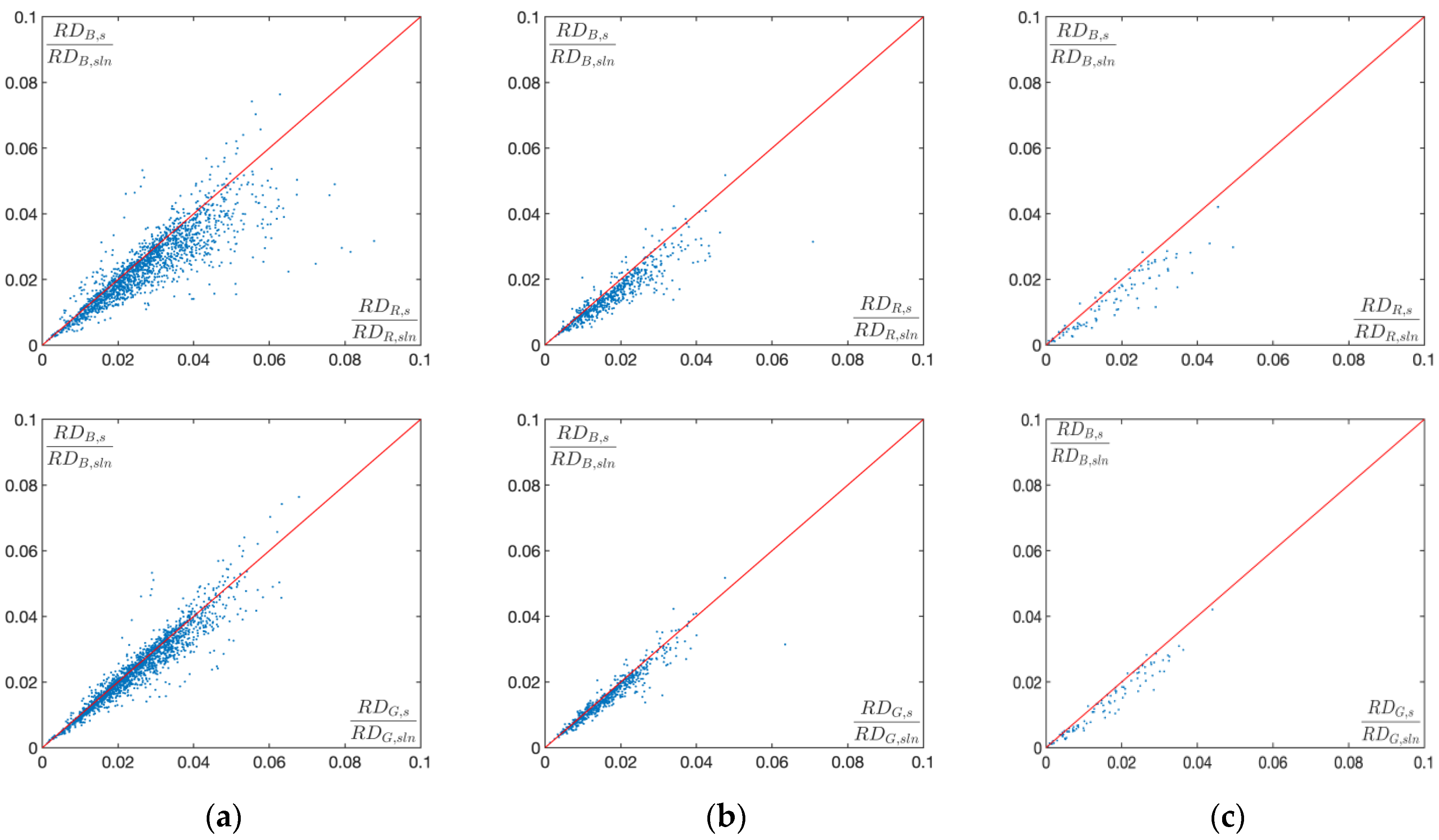
As shown in Figure 2, columns (a), (b) and (c) are the R D c , s R D c , s l n statistics on the three datasets of NUS, Gehler-Shi and SFU, respectively. The scatter points in each sub-graph represent the R D c , s R D c , s l n information of one of the three RGB channels of a picture. For example, the three plots in the first column of Figure 2 depict the 1737 ratios of R D c , s and R D c , s l n in each of the three color channels in the NUS dataset, where each discrete point corresponds to a picture in the NUS dataset, and R D c , s R D c , s l n with c { R , G , B } . In detail, R D R , s R D R , s l n denotes the ratio of R D c , s and R D c , s l n in red color channel of the image.
As we can see from Figure 2, it is obvious that most of the scattered points are distributed along the diagonal line. Therefore, we can get the formula:
R D R , s R D R , s l n = R D G , s R D G , s l n = R D B , s R D B , s l n = k
where k is a constant. For uniform illumination, the light source color can be computed by:
Ω f c , X ( x ) 1 J ξ f c , X ( x ) f c , X ( x j , m a x ) d x d j = e c R c X ( x ) d x 1 J ξ e c · R c , j X ( x ) e c · R c , j X ( x j , m a x ) d x d j = e c R c X ( x ) d x 1 J ξ L c , X , j ( x ) d x d j = k e c
Based on the above inference. Given a color-biased image f c ( x ) as input, R can be determined by Equation (8), k functions as a scaling coefficient that varies according to the scene observed. Given that k is the same for all color channels c { R , G , B } , based on Equation (11) and Equation (3), we don’t have to find the actual value of k because it can be negated by using the normalized form of e c as the final result of the illumination.

2.3. Expanded into a Unified Framework

In this section, we will show than we propose a new framework that can incorporate several important statistics-based color constancy algorithms (Grey-World, maximum RGB, Grey-Edge, etc.).
Our proposed method, like the previous framework Equation (1), can well be modified to merge into the Minkowski norm:
( ( f c , X n , σ ( x ) ) p d x 1 J ξ ( L c , X , j n , σ ( x ) ) p d x d j ) 1 p = k e c n , p , σ , J
where
f c , X n , σ ( x ) = | n f c σ ( x ) x n | = | n f c ( x ) G σ x n |
L c , X , j n , σ ( x ) = f c , X σ , n ( x ) f c , X σ , n ( x j , m a x )
f c , X n , σ ( x ) denotes the spatial derivatives of order n . The Gaussian filter G σ with standard deviation σ is also introduced in order to exploit the local correlation. The Minkowski norm p determines the relative weights of the multiple measures used to estimate the final illuminant color.
What is more, Table 1 demonstrates that both Grey-World, White-Patch, Grey-Edge, and Local-Surface methods are the extreme case of Equation (13). For example, for color constancy method 2nd order Local-Edge, ( ( f c , X 2 , σ ( x ) ) p d x 1 J ξ ( L c , X , j 2 , σ ( x ) ) p d x d j ) 1 p = k e c , e c = e c 2 , p , σ , J , that is, J represents the total number of the local regions inside the image, the spatial derivatives is 2, p represents Minkowski norm and σ represents the standard deviation of the Gaussian filter. Similarly, the remaining color constancy methods in Table 1 can also be incorporated into the unified framework we propose.

3. Experimental Results

The previous section provided a generic formulation of color illuminant estimates using low-level image features. In this section, the proposed approach is evaluated on four benchmark datasets, one indoor light source dataset [32], two for the real-world dataset (SFU indoor dataset and Grey-ball dataset) [13,30], and one for the HDR light source dataset [33]. The light source color of the scene is given as extra data for both datasets.
The angular error is used as the color constancy error metric [34]:
a n g u l a r   e r r o r = c o s 1 ( e l · e e )
where the e l indicates the actual light source and the e e indicates the estimated light source. Smaller angular errors indicate more accurate color constancy results. In order to evaluate the proposed algorithm more objectively, five metrics including median, mean, trimean, max angular error are used to measure the accuracy of the color constancy of the method.
The proposed method in the paper is a low-level based method, so we compared it to the following low-level based methods: Inverse-Intensity Chromaticity Space (IICS) [22], Grey-World [24], White-Patch [25], Shade of Grey [35], General Grey World [34], 1-st order Grey-Edge, 2-nd order Grey-Edge [26], Local Surface Reflectance [29]. It also includes the most advanced methods available, such as pixel-based Gamut Mapping [7], edge-based Gamut Mapping [36], Spatio-Spectral Statistics [37], Weighted Grey Edge [27], SVR Regression [38], Natural Image Statistics [18], Exemplar-based method [16], Bayesian [15], and Thin-plate Spline Interpolation [39].

3.1. Parameter Setting and Analysis

As previously stated in Section 2, the proposed method should select the best parameter values. In our model there are a total of four variables, because of the computational limitation, only 1st-order and 2nd-order are discussed, and the remaining variables are only three, which are Minkowski norm p , scale σ , and number of the local regions J . Empirically, we traverse the indoor image dataset to determine the optimal parameters. The final selected parameters are shown in Table 2. As shown in Table 2, both Minkowski norm p and the local regions J adopt the same setting in both 1st-order Local edge and 2nd-order Local edge methods. We set scale σ = 4 and scale σ = 6 in the 1st-order Local edge and 2nd-order Local edge color constancy methods, respectively.

3.2. Indoor Dataset

The angular error results of various models on the SFU indoor dataset are presented in Table 3. A total of 321 linear photos were captured in the laboratory under 11 various illumination conditions in the SFU indoor dataset [32].
It can be seen from Table 3 that our model performed well when compared to other models on a variety of measures. Specifically, our proposed 2nd-order Local Edge color constancy method achieves the smallest angular error on the four metrics of median, mean, trimean and best-25%, and the proposed 1st-order Local Edge method on the worst-25% metric, it achieves better results than the comparison algorithm. Table 3 shows that the proposed color constancy method can achieve more accurate lighting color estimation results than the comparison algorithm in indoor lighting environments.

3.3. Real-World Dataset

The Gehler-Shi dataset includes 568 linear natural photos [15,30], all of which were captured in RAW format with a DSLR camera, with no color correction. As in many prior studies, the 24 patch color checkboard in every image of the dataset was disguised for illuminant estimation.
Our approaches were then tested on the SFU Grey-Ball dataset [13], which comprises 11,346 non-linear photos. This dataset has been treated in camera using complicated processing, making it impossible to derive an exact illuminant estimate. Before the experiment, we masked out the gray balls in each photo for unbiased evaluation.
Table 4 shows the results on this color check dataset, and Table 5 lists the results of the SFU grey-ball dataset. In general, among all models, our method shows the best color constancy accuracy. As can be seen from Table 4, the 2nd-order Local edge method we proposed achieved the lowest values on the five metrics of median, mean, trimean, best-25% and worst-25%. Lower values for the above five metrics indicate more accurate color constancy. Therefore, the 2nd-order Local edge method we proposed is superior to Grey-World, White-patch, Shade of Grey, Grey-Edge, Local Surface Reflectance, Pixel-based Gamut, Edge-based Gamut on the Gehler-Shi dataset test set, SVR Regression, Bayesian, Exemplar-based and NIS color constancy methods. Specifically, it can be seen from Table 5 that on the SFU Grey-Ball dataset, our proposed 2nd-order Local edge method achieves optimal results on the three metrics of mean, best-25% and worst-25%. And it is only 0.36 higher than the best performing Exemplar-based method on the median metric.
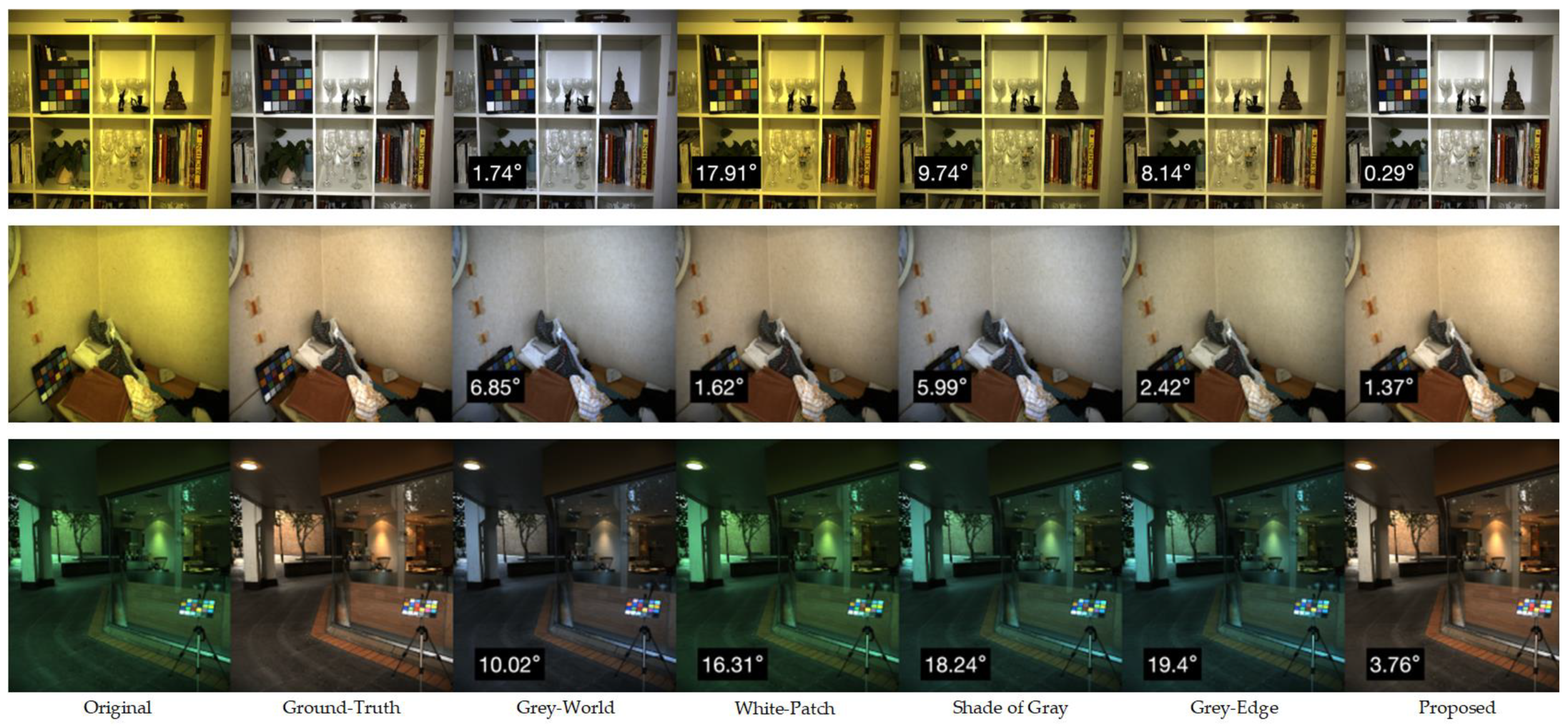
Figure 3 demonstrates the results on sample photos from the color checker dataset. It can be seen from Figure 3 that the proposed color constancy method can well restore the real color of the scene on the Gehler-Shi test data set. For the scenes shown in the first and third rows in Figure 3, the White-Patch, Shade of Gray and Gray-Edge methods can hardly restore the actual color of the scene, and the results have no obvious improvement compared to the original input. Gray-World has achieved better color constancy results than the above methods in all scenes, but it still has a certain degree of color cast. Our proposed method achieves the smallest angular error on all test scenarios.

3.4. SFU HDR Dataset

Our approach was then tested on a dataset with an HDR light source [33], which includes 105 high-quality images captured under indoor and outdoor light sources.
The performance statistics for several methods on the SFU HDR dataset are shown in Table 6. When compared to other models on this dataset, our model performs well on a variety of metrics. It can be seen from Table 6 that on the SFU HDR image dataset, the 2nd-order Local edge method we proposed achieved the best results on the three metrics of median, mean and worst-25%, and the proposed 1st-order Local edge algorithm achieves as good results as the 2nd-order Local edge on the median metric. The proposed methods are significantly better than the second-ranked Grey-Edge algorithm. Table 6 shows that the color constancy method we proposed can also accurately restore the true color of the scene in the HDR scene with rich light sources both indoors and outdoors.

4. Conclusions

In this paper, inspired by the Gray-Edge hypothesis, our statistical experiments on the three public datasets of NUS, Gehler-Shi and SFU show that the ratio of the global sum of reflection differences to the global sum of locally normalized reflection differences is achromatic. Based on the above conclusion, we propose a new method for more accurate color constancy. Qualitative and quantitative results of the proposed color constancy method on multiple test datasets containing different lighting scenarios demonstrate its effectiveness. In particular, the experimental results on the HDR test set show that the color constancy method proposed by us is superior to the comparison algorithm, showing that the proposed method can restore the actual color more accurately for different scenes. Additionally, we propose a new framework that can incorporate current mainstream statistics-based color constancy methods (Gray-World, Max-RGB, Gray-Edge, etc.) into the proposed framework. A limitation of our research work is that the four parameters in the proposed color constancy algorithm are empirical rather than adaptive. Our future research work is to combine the statistical information of the image with the convolutional neural network to design a network structure with more accurate color constancy.

Author Contributions

Conceptualization, M.Y. and Y.H.; methodology, M.Y.; software, M.Y.; validation, M.Y., Y.H. and H.Z.; formal analysis, M.Y.; investigation, M.Y.; resources, M.Y.; data curation, M.Y.; writing—original draft preparation, M.Y.; writing—review and editing, H.Z.; visualization, M.Y.; supervision, Y.H.; project administration, Y.H.; funding acquisition, Y.H. All authors have read and agreed to the published version of the manuscript.

Funding

This research was funded by the National Nature Science Foundation of China, grant number 62073210.

Data Availability Statement

The data that support the findings of this study are available on request from the corresponding author.

Conflicts of Interest

The authors declare no conflict of interest.

References

  1. Foster, D.H. Color constancy. Vision Res. 2011, 51, 674–700. [Google Scholar] [CrossRef] [PubMed]
  2. Laakom, F.; Passalis, N.; Raitoharju, J.; Nikkanen, J.; Tefas, A.; Iosifidis, A.; Gabbouj, M. Bag of color features for color constancy. IEEE Trans. Image Process. 2020, 29, 7722–7734. [Google Scholar] [CrossRef]
  3. Ding, X.; Wang, Y.; Fu, X. An image dehazing approach with adaptive color constancy for poor visible conditions. IEEE Geosci. Remote. Sens. 2021, 19, 1–5. [Google Scholar] [CrossRef]
  4. Mastour, N.; Ramachandran, K.; Ridene, S.; Daoudi, K.; Gaidi, M. Tailoring the optical band gap of In–Sn–Zn–O (ITZO) nanostructures with co-doping process on ZnO crystal system: An experimental and theoretical validation. Eur. Phys. J. Plus 2022, 137, 1137. [Google Scholar] [CrossRef]
  5. Mastour, N.; Jemaï, M.; Ridene, S. Calculation of ground state and Hartree energies of MoS2/WSe2 assembled type II quantum well. Micro Nanostruct. 2022, 171, 207417. [Google Scholar] [CrossRef]
  6. Ridene, S. Mid-infrared emission in InxGa1−xAs/GaAs T-shaped quantum wire lasers and its indium composition dependence. Infrared Phys. Technol. 2018, 89, 218–222. [Google Scholar] [CrossRef]
  7. Forsyth, D. A novel algorithm for color constancy. Int. J. Comput. Vis. 1990, 5, 5–36. [Google Scholar] [CrossRef]
  8. Barnard, K.; Martin, L.; Coath, A.; Funt, B. A comparison of computational color constancy algorithms—Part II: Experiments with image data. IEEE Trans. Image Process. 2002, 11, 985–996. [Google Scholar] [CrossRef] [Green Version]
  9. Finlayson, G.; Hordley, S. Gamut constrained illumination estimation. Int. J. Comput. Vis. 2006, 67, 93–109. [Google Scholar] [CrossRef] [Green Version]
  10. Banic, N.; Loncaric, S. Color cat: Remembering colors for illumination estimation. IEEE Signal Process. Lett. 2014, 22, 651–655. [Google Scholar] [CrossRef]
  11. Finlayson, G.D. Corrected-moment illuminant estimation. In Proceedings of the IEEE International Conference on Computer Vision, Sydney, Australia, 1–8 December 2013. [Google Scholar]
  12. Cardei, V.C.; Funt, B.; Barnard, K. Estimating the scene illumination chromaticity by using a neural network. J. Opt. Soc. Am. A 2002, 19, 2374–2386. [Google Scholar] [CrossRef] [Green Version]
  13. Ciurea, F.; Funt, B. A large image database for color constancy research. In Proceedings of the Color and Imaging Conference, Scottsdale, AZ, USA, 4–7 November 2003. [Google Scholar]
  14. Brainard, D.H.; Freeman, W.T. Bayesian color constancy. J. Opt. Soc. Am. A 1997, 14, 1393–1411. [Google Scholar] [CrossRef]
  15. Gehler, P.V.; Rother, C.; Blake, A.; Minka, T.; Sharp, T. Bayesian color constancy revisited. In Proceedings of the IEEE Conference on Computer Vision and Pattern Recognition, Anchorage, AK, USA, 23–28 June 2008. [Google Scholar]
  16. Joze, H.R.V.; Drew, M. Exemplar-based colour constancy and multiple illumination. IEEE Trans. Pattern Anal. Mach. Intell. 2013, 36, 860–873. [Google Scholar] [CrossRef]
  17. Gao, S.; Yang, K.; Li, C.; Li, Y. A color constancy model with double-opponency mechanisms. In Proceedings of the IEEE International Conference on Computer Vision, Sydney, Australia, 1–8 December 2013. [Google Scholar]
  18. Gijsenij, A.; Gevers, T. Color constancy using natural image statistics and scene semantics. IEEE Trans. Pattern Anal. Mach. Intell. 2011, 33, 687–698. [Google Scholar] [CrossRef]
  19. Bianco, S.; Schettini, R. Color constancy using faces. In Proceedings of the Conference on Computer Vision and Pattern Recognition, Providence, RI, USA, 16–21 June 2012. [Google Scholar]
  20. Van De Weijer, J.; Schmid, C.; Verbeek, J. Using high-level visual information for color constancy. In Proceedings of the Conference on Computer Vision, Minneapolis, MN, USA, 17–22 June 2007. [Google Scholar]
  21. Lee, H.C. Method for computing the scene-illuminant chromaticity from specular highlights. J. Opt. Soc. Am. A 1986, 3, 1694–1699. [Google Scholar] [CrossRef]
  22. Tan, R.T.; Nishino, K.; Ikeuchi, K. Color constancy through inverse-intensity chromaticity space. J. Opt. Soc. Am. A 2004, 21, 321–334. [Google Scholar] [CrossRef] [Green Version]
  23. Xiao, J.; Gu, S.; Zhang, L. Multi-domain learning for accurate and few-shot color constancy. In Proceedings of the IEEE/CVF Conference on Computer Vision and Pattern Recognition, Seattle, WA, USA, 13–19 June 2020. [Google Scholar]
  24. Buchsbaum, G. A spatial processor model for object colour perception. J. Frankl. Inst. 1980, 310, 1–26. [Google Scholar] [CrossRef]
  25. Land, E.H. The retinex theory of color vision. Sci. Am. 1977, 237, 108–129. [Google Scholar] [CrossRef]
  26. Van De Weijer, J.; Gevers, T.; Gijsenij, A. Edge-based color constancy. IEEE Trans. Image Process. 2010, 16, 2207–2214. [Google Scholar] [CrossRef] [Green Version]
  27. Gijsenij, A.; Gevers, T.; Van De Weijer, J. Improving color constancy by photometric edge weighting. IEEE Trans. Pattern Anal. Mach. Intell. 2011, 34, 918–929. [Google Scholar] [CrossRef]
  28. Schiller P, H. Parallel information processing channels created in the retina. Proc. Natl. Acad. Sci. USA 2010, 107, 17087–17094. [Google Scholar] [CrossRef] [PubMed] [Green Version]
  29. Gao, S.; Han, W.; Yang, K.; Li, C.; Li, Y. Efficient color constancy with local surface reflectance statistics. In Proceedings of the European Conference on Computer Vision, Zurich, Switzerland, 6–12 September 2014. [Google Scholar]
  30. Shi, L.; Funt, B. Re-Processed Version of the Gehler Color Constancy Dataset of 568 Images. Available online: http://www.cs.sfu.ca/~colour/data/ (accessed on 7 May 2014).
  31. Cheng, D.; Prasad, D.K.; Brown, M.S. Illuminant estimation for color constancy: Why spatial-domain methods work and the role of the color distribution. J. Opt. Soc. Am. A 2014, 31, 1049–1058. [Google Scholar] [CrossRef] [PubMed] [Green Version]
  32. Barnard, K.; Martin, L.; Funt, B.; Coath, A. A data set for color research. Color. Res. Appl. 2002, 27, 147–151. [Google Scholar] [CrossRef]
  33. Funt, B.; Shi, L. The rehabilitation of MaxRGB. In Proceedings of the Eighteenth Color Imaging Conference, Simon Fraser University, San Antonio, TX, USA, 1 November 2020. [Google Scholar]
  34. Gijsenij, A.; Gevers, T.; Van De Weijer, J. Computational color constancy: Survey and experiments. IEEE Trans. Image Process. 2011, 20, 2475–2489. [Google Scholar] [CrossRef]
  35. Finlayson, G.D.; Trezzi, E. Shades of gray and colour constancy. In Proceedings of the Color and Imaging Conference, Scottsdale, AZ, USA, 9–12 November 2004. [Google Scholar]
  36. Gijsenij, A.; Gevers, T.; Van De Weijer, J. Generalized gamut mapping using image derivative structures for color constancy. Int. J. Comput. Vis. 2010, 86, 127–139. [Google Scholar] [CrossRef] [Green Version]
  37. Chakrabarti, A.; Hirakawa, K.; Zickler, T. Color constancy with spatio- spectral statistics. IEEE Trans. Pattern Anal. Mach. Intell. 2012, 34, 1509–1519. [Google Scholar] [CrossRef] [Green Version]
  38. Xiong, W.; Funt, B. Estimating illumination chromaticity via support vector regression. J. Imaging Sci. Technol. 2006, 50, 341–348. [Google Scholar] [CrossRef] [Green Version]
  39. Shi, L.; Xiong, W.; Funt, B. Illumination estimation via thin-plate spline interpolation. J. Opt. Soc. Am. A 2011, 28, 940–948. [Google Scholar] [CrossRef] [Green Version]
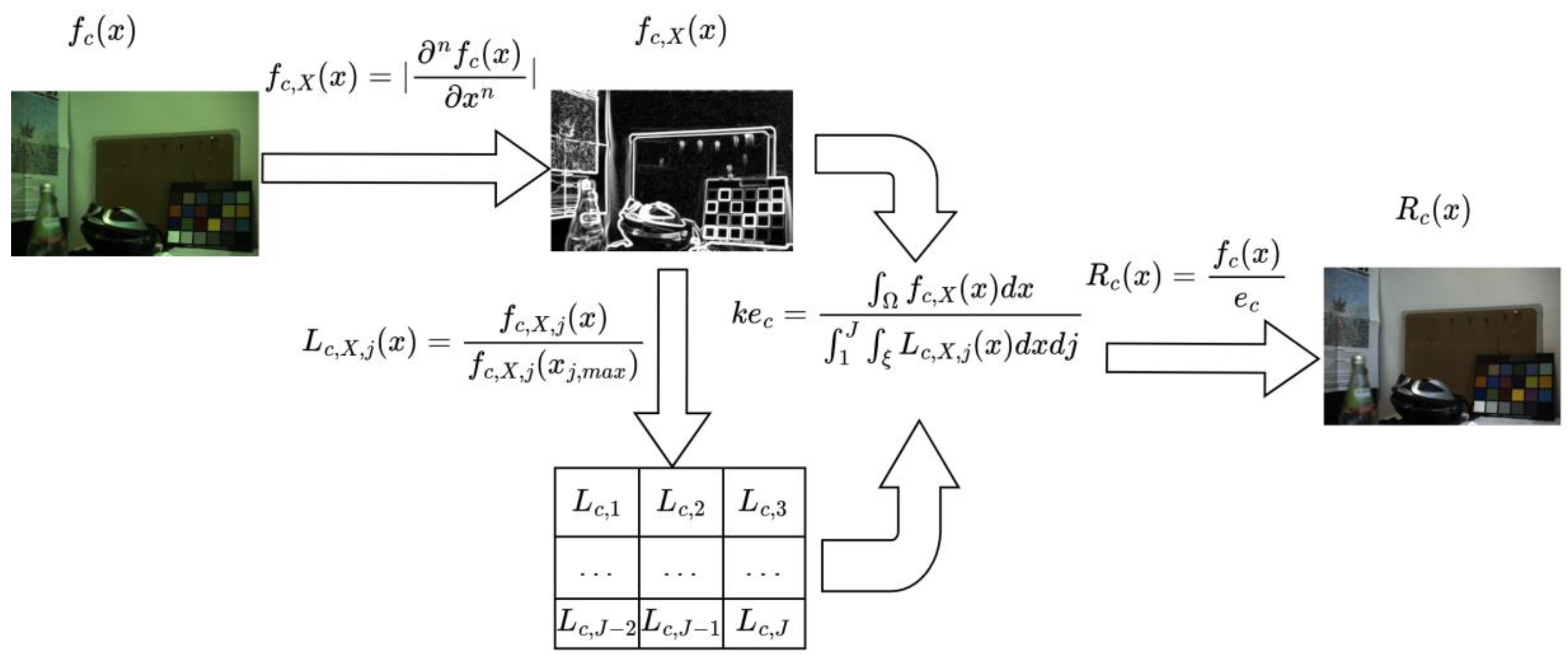
Figure 1. The flowchart of the proposed color constancy approach.
Electronics 12 01396 g001
Figure 2. Each point in the scatter plots represents the ratio of statistical values between R D c , s and R D c , s l n in the three color channels for an image. For example, the graph at the top of column (a) represents the R D c , s R D c , s l n information of all pictures in the NUS dataset in the two channels of green and red (i.e., R D G , s R D G , s l n and R D R , s R D R , s l n ). These plots indicate that most of these scatter points are distributed along the diagonal line (the red solid line). (a) The ratio of statistical values between R D c , s and R D c , s l n in the three color channels for an image in NUS dataset; (b) The ratio of statistical values between R D c , s and R D c , s l n in the three color channels for an image in Gehler-Shi dataset; (c) The ratio of statistical values between R D c , s and R D c , s l n in the three color channels for an image in SFU dataset.
Electronics 12 01396 g002aElectronics 12 01396 g002b
Figure 3. Color constancy results of Gray-World, White-Patch, Shades of Grey, Grey-Edge, and proposed on Gehler-Shi test dataset. The angular error is indicated in the left bottom corner.
Electronics 12 01396 g003
Table 1. A summary of the different illuminant estimations methods.
MethodsSymbolEquation
Grey-World e c 0 , 1 , 0 , N ( f c ( x ) d x ) = k e c
White-Patch e c 0 , , 0 , N ( | f c ( x ) | d x ) 1 = k e c
Grey-Edge e c 1 , p , σ , N ( | f c , X σ ( x ) | p d x ) 1 p = k e c
Local-Surface e c 0 , 1 , 0 , J ( | f c ( x ) | d x 1 J ξ | L c , j ( x ) | d x d j ) = k e c
Local-Edge e c 1 , p , σ , J ( ( f c , X 1 , σ ( x ) ) p d x 1 J ξ ( L c , X , j 1 , σ ( x ) ) p d x d j ) 1 p = k e c
2nd order Local-Edge e c 2 , p , σ , J ( ( f c , X 2 , σ ( x ) ) p d x 1 J ξ ( L c , X , j 2 , σ ( x ) ) p d x d j ) 1 p = k e c
Table 2. Parameter settings in the proposed 1st-order Local edge and 2nd-order Local edge color constancy methods. Noted that the parameters are empirical.
MethodsMinkowski ( p ) Scale ( σ ) Region Number ( J )
1st-order Local edge10416
2nd-order Local edge10616
Table 3. The performance of different color constancy methods on the SFU indoor dataset.
MethodsMedianMeanTrimeanBest-25%Worst-25%
IICS8.215.512.02.240.0
Grey-World7.09.88.10.9023.3
White-Patch6.59.17.61.820.9
Shade of Grey3.76.45.00.616.4
General Grey World3.35.44.10.513.7
1st-order Grey-Edge3.205.64.21.014.0
2nd-order Grey-Edge2.75.24.31.213.7
Local Surface Reflectance2.45.74.10.515
Pixel-based Gamut2.33.72.70.59.3
Edge-based Gamut2.33.92.80.616.08
Bayesian3.672.732.910.828.21
NIS3.712.602.840.798.47
19-Edge Corrected-moment2.02.62.250.687.08
Proposed 1st-order Local Edge2.02.522.310.466.78
Proposed 2nd-order Local Edge1.92.502.230.456.79
Table 4. Performance of different color constancy methods on the Gehler-Shi dataset.
MethodsMedianMeanTrimeanBest-25%Worst-25%
IICS13.613.613.49.518.0
Grey-World6.36.46.32.310.6
White-patch5.77.56.71.516.1
Shade of Grey4.04.94.41.110.2
General Grey World3.54.74.01.010.2
1st-order Grey-Edge4.75.95.41.611.9
2nd-order Grey-Edge4.55.34.91.910.0
Local Surface Reflectance2.63.42.90.87.2
Pixel-based Gamut2.44.23.30.511.2
Edge-based Gamut5.66.76.02.013.5
SVR Regression6.78.17.43.314.9
Bayesian3.54.84.11.310.5
Exemplar-based2.32.92.50.86.0
NIS3.14.23.51.09.2
19-Edge Corrected-moment2.02.82.250.687.08
Proposed 1st-order Local edge1.82.042.310.665.89
Proposed 2nd-order Local edge1.751.972.280.655.80
Table 5. Performance of different color constancy methods on the SFU Grey-Ball dataset.
MethodsMedianMeanBest-25%Worst-25%
IICS5.66.61.813.3
Grey-World7.07.92.215.2
White-Patch5.36.81.214.7
Shade of Grey5.36.11.811.9
General Grey World5.36.11.811.9
1st-order Grey-Edge4.75.91.611.9
2nd-order Grey-Edge4.86.11.612.4
Local Surface Reflectance5.16.0-11.9
Pixel-based Gamut5.87.11.714.7
Edge-based Gamut5.86.81.913.5
Exemplar-based3.44.41.09.4
NIS3.95.21.211.1
Proposed 1st-order Local edge3.84.360.98.89
Proposed 2nd-order Local edge3.764.320.878.89
Table 6. Performance of different color constancy methods on the SFU HDR image dataset.
MethodsMedianMeanWorst-25%
Grey-World7.48.019.5
White-Patch3.96.3-
Shade of Grey3.95.712.9
Grey-Edge3.86.013.8
Proposed 1st-order Local edge2.94.610.6
Proposed 2nd-order Local edge2.94.510.4
Disclaimer/Publisher’s Note: The statements, opinions and data contained in all publications are solely those of the individual author(s) and contributor(s) and not of MDPI and/or the editor(s). MDPI and/or the editor(s) disclaim responsibility for any injury to people or property resulting from any ideas, methods, instructions or products referred to in the content.