

Influence of Different Data Interpolation Methods for Sparse Data on the Construction Accuracy of Electric Bus Driving Cycle


Abstract
1. Introduction
2. Data and Methods
2.1. Original Data Collection
2.2. Data Preprocessing Methods
2.2.1. Micro-Trip Segmentation
2.2.2. Sparse Data Interpolation
2.2.3. Characteristic Parameters Extraction
2.3. Principal Component Analysis Method
2.3.1. Theoretical Basis
2.3.2. Analytical Process
2.4. K-means Clustering Method
2.4.1. Theoretical Basis
2.4.2. Analytical Process
2.5. Condition Synthesis Method
2.5.1. Determination of Duration and Number of Segments
2.5.2. Fragment Selection
2.5.3. Short Travel Segment Splicing
3. Results
3.1. Influence of Different Interpolation Methods on Principal Components
3.2. Influence of Different Interpolation Methods on K-means Clustering
3.2.1. Silhouette Coefficient
3.2.2. Results of Clustering Quantity
3.2.3. Scatter Plot Results
3.2.4. Represents Short Trip Results
3.3. The Influence of Different Interpolation Methods on the Synthesis of Working Conditions
3.3.1. Number of Short Travel Segments
3.3.2. Synthetic Condition
4. Discussion
4.1. Comparative Analysis of Three Synthesis Conditions
4.2. Comparison between Optimal Synthesis Condition and Standard Condition
5. Conclusions
- (1)
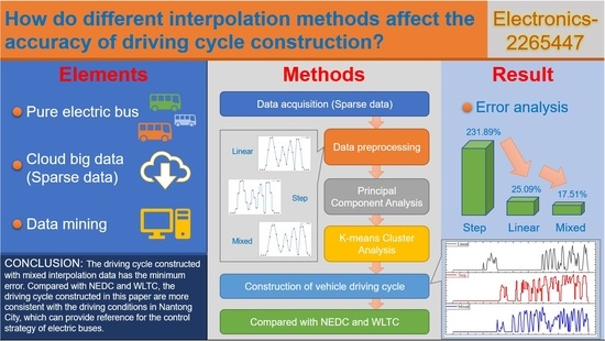
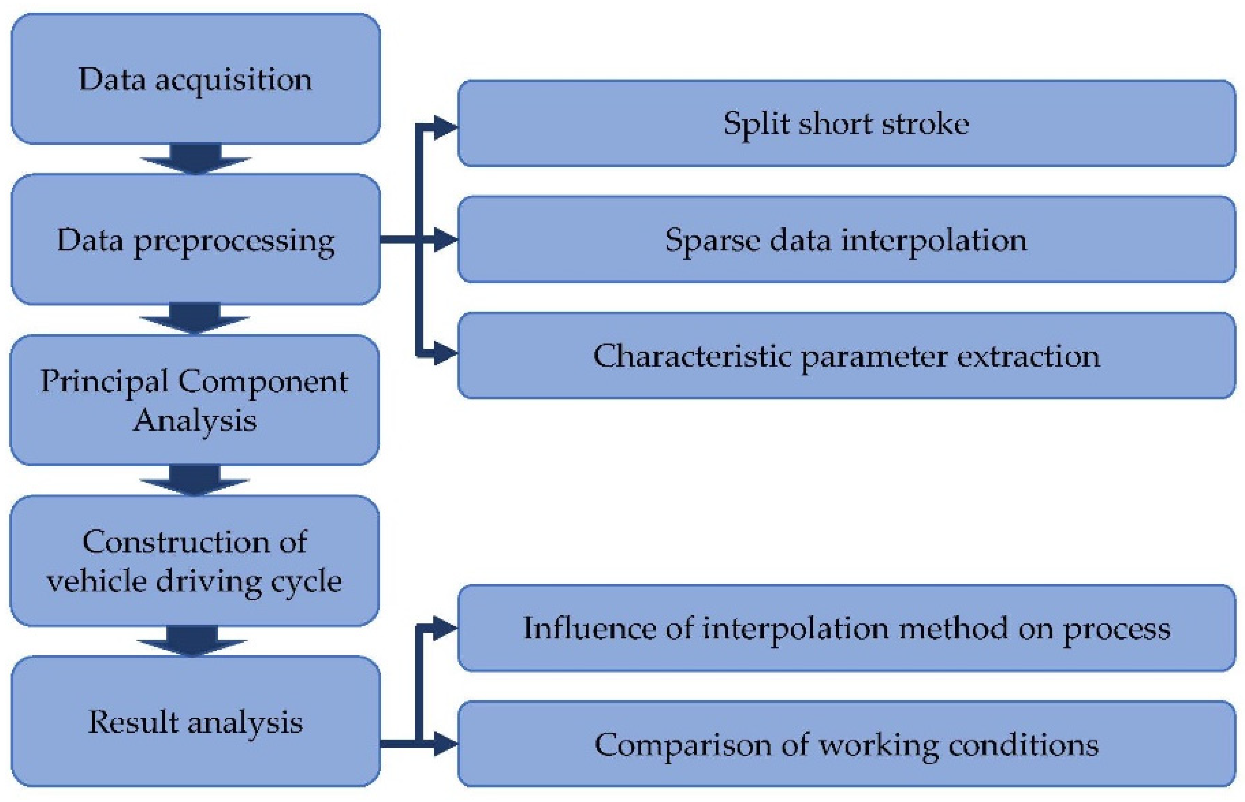
- Three different interpolation methods, linear interpolation, step interpolation and mixed interpolation, were used to preprocess the collected data, and 1870 short-stroke fragments were extracted from the data. The feature parameter matrix will be reduced and classified using the principal component analysis method and K-means clustering algorithm. The silhouette index will be used as the standard for measuring the clustering results. According to the clustering results, sports segment libraries and idle segment libraries of different categories were established, from which the most frequent duration segments were selected, and the segment closest to the clustering center was selected from the corresponding duration segments to construct the representative bus driving conditions of Nantong city.
- (2)
- The step interpolation method has a poor processing effect, and the relative error between the synthetic conditions and the measured data is the largest, whose average value is 231.89%, which cannot meet the development requirements. The linear interpolation method has a general processing effect, and the relative error between the synthetic conditions and the measured data is large, with an average value of 25.09%, which does not meet the development requirements. The mixed interpolation method based on linear interpolation and cubic spline interpolation has a good processing effect. The average relative error between the synthetic conditions and the measured data is 15.71%, and the relative error of 10 of the 12 characteristic parameters is less than 15%. Therefore, the working conditions constructed by the mixed interpolation method proposed in this paper basically meet the development requirements. It can accurately reflect the characteristics of the sample population.
- (3)
- The average running speed of buses in Nantong city is low, the idle time ratio is high and the maximum speed is low. Compared with NEDC and WLTC, the average running speed, the maximum speed and the idle time ratio of buses in Nantong city are significantly different, with the average relative error reaching 71.53% and 85.37%, respectively. The comparison results show that WLTC driving conditions are difficult to accurately reflect the actual traffic conditions of buses in Nantong city. In order to develop better energy management strategies and vehicle emission standards, it is necessary to consider the influence of regional differences and construct representative driving conditions in line with the actual local driving conditions.
6. Patents
Author Contributions
Funding
Institutional Review Board Statement
Informed Consent Statement
Data Availability Statement
Acknowledgments
Conflicts of Interest
Nomenclature
| Parameter | Meaning Represented |
| maximum speed | |
| average speed | |
| average driving speed | |
| speed standard deviation | |
| maximum acceleration | |
| minimum deceleration speed | |
| average acceleration | |
| average deceleration speed | |
| acceleration time ratio | |
| deceleration time ratio | |
| idle speed time ratio | |
| uniform speed time ratio | |
| total length of the short journey | |
| driving distance | |
| observation matrix | |
| value of the jth characteristic parameter of the ith micro-trip | |
| normalized matrix | |
| original observation matrix characteristic parameters of the mean | |
| variance of the original observation matrix | |
| correlation coefficient matrix | |
| contribution rate | |
| Euclidean distance | |
| error sum of squares criterion function | |
| time of class i condition in the final synthesis condition | |
| duration of representative working conditions | |
| total duration of all operating conditions | |
| number of micro-trips in class i | |
| running time of the j-micro-trip segment in class i | |
| BEVs | battery electric vehicles |
| NEDC | new European driving cycle |
| WLTC | worldwide harmonized light vehicles test cycle |
| SOC | state of charge |
| PCA | principal components analysis |
| SVM | support vector machines |
| GMM | gaussian mixture model |
| DBSCAN | density-based spatial clustering of applications with noise |
Appendix A

| Serial Number | Initial Characteristic Parameter | ||
|---|---|---|---|
| Total | Percentage of Variance | Cumulative (%) | |
| 1 | 5.674 | 47.284 | 47.284 |
| 2 | 1.960 | 16.334 | 63.618 |
| 3 | 1.662 | 13.849 | 77.467 |
| 4 | 1.173 | 9.779 | 87.246 |
| 5 | 0.792 | 6.602 | 93.848 |
| 6 | 0.245 | 2.043 | 95.890 |
| 7 | 0.195 | 1.623 | 97.513 |
| 8 | 0.149 | 1.243 | 98.757 |
| 9 | 0.066 | 0.547 | 99.303 |
| 10 | 0.058 | 0.480 | 99.784 |
| 11 | 0.026 | 0.216 | 99.99999… |
| 12 | 6.992 × 10⁻¹⁵ | 5.827 × 10⁻¹⁴ | 100.000 |
| Serial Number | F1 | F2 | F3 | F4 | Y1 | Y2 | Y3 | Y4 |
|---|---|---|---|---|---|---|---|---|
| 1 | −1.65 | −0.05 | 0.72 | −0.44 | −3.93 | −0.01 | 0.92 | −0.48 |
| 2 | 0.59 | 1.01 | 1.46 | −0.17 | 1.4 | 1.42 | 1.88 | −0.19 |
| 3 | −1.23 | −0.01 | −0.54 | −0.61 | −2.93 | −0.02 | −0.7 | −0.67 |
| … | … | … | … | … | … | … | … | … |
| 1869 | −1.38 | 0.41 | −0.74 | −0.51 | −3.29 | 0.58 | −0.95 | −0.55 |
| 1870 | −3.10 | 2.22 | 2.43 | 0.37 | −7.39 | 3.11 | 3.13 | 0.4 |
| Serial Number | Initial Characteristic Parameter | ||
|---|---|---|---|
| Total | Percentage of Variance | Cumulative (%) | |
| 1 | 6.014 | 50.120 | 50.120 |
| 2 | 2.608 | 21.735 | 71.855 |
| 3 | 1.342 | 11.180 | 83.035 |
| 4 | 0.950 | 7.915 | 90.951 |
| 5 | 0.334 | 2.786 | 93.737 |
| 6 | 0.236 | 1.965 | 95.702 |
| 7 | 0.194 | 1.613 | 97.315 |
| 8 | 0.148 | 1.230 | 98.545 |
| 9 | 0.077 | 0.639 | 99.184 |
| 10 | 0.073 | 0.612 | 99.796 |
| 11 | 0.024 | 0.204 | 99.99999… |
| 12 | 2.013 × 10⁻¹⁵ | 1.678 × 10⁻¹⁴ | 100.000 |
| Serial Number | F1 | F2 | F3 | Y1 | Y2 | Y3 |
|---|---|---|---|---|---|---|
| 1 | −1.49 | 0.79 | −1.09 | −3.66 | 1.27 | −1.17 |
| 2 | 0.92 | 1.01 | −0.14 | 2.25 | 1.63 | −0.16 |
| 3 | −1.25 | 0.27 | −0.97 | −3.07 | 0.43 | −1.12 |
| … | … | … | … | … | … | … |
| 1869 | −1.20 | 1.06 | −0.09 | −2.95 | 1.7 | −0.11 |
| 1870 | −2.22 | 2.48 | 0.78 | −5.46 | 4.01 | 0.91 |
References
- Jiang, N.; Wang, X.; Kang, L. A Novel Power Distribution Strategy and Its Online Implementation for Hybrid Energy Storage Systems of Electric Vehicles. Electronics 2023, 12, 301. [Google Scholar] [CrossRef]
- Zhang, C.; Guo, Q.; Li, L.; Wang, M.; Wang, T. System Efficiency Improvement for Electric Vehicles Adopting a Permanent Magnet Synchronous Motor Direct Drive System. Energies 2017, 10, 2030. [Google Scholar] [CrossRef]
- Hong, S.; Kang, M.; Park, H.; Kim, J.; Baek, J. Real-Time State-of-Charge Estimation Using an Embedded Board for Li-Ion Batteries. Electronics 2022, 11, 2010. [Google Scholar] [CrossRef]
- Zhang, Q.; Shaopeng, T.; Xinyan, L. Recent Advances and Applications of AI-Based Mathematical Modeling in Predictive Control of Hybrid Electric Vehicle Energy Management in China. Electronics 2023, 12, 445. [Google Scholar] [CrossRef]
- Wang, X.; Ye, P.; Zhang, Y.; Ni, H.; Deng, Y.; Lv, S.; Yuan, Y.; Zhu, Y. Parameter Optimization Method for Power System of Medium-Sized Bus Based on Orthogonal Test. Energies 2022, 15, 7243. [Google Scholar] [CrossRef]
- Cheng, Y.; Xu, G.; Chen, Q. Research on Energy Management Strategy of Electric Vehicle Hybrid System Based on Reinforcement Learning. Electronics 2022, 11, 1933. [Google Scholar] [CrossRef]
- Zhao, X.; Zhao, X.; Yu, Q.; Ye, Y.; Yu, M. Development of a representative urban driving cycle construction methodology for electric vehicles: A case study in Xi’an. Transp. Res. Part D Transp. Env. 2020, 81, 102279. [Google Scholar] [CrossRef]
- Hongwen, H.; Jinquan, G.; Jiankun, P.; Huachun, T.; Chao, S. Real-time global driving cycle construction and the application to economy driving pro system in plug-in hybrid electric vehicles. Energy 2018, 152, 95–107. [Google Scholar] [CrossRef]
- Amirjamshidi, G.; Roorda, M.J. Development of simulated driving cycles for light, medium, and heavy duty trucks: Case of the Toronto Waterfront Area. Transp. Res. Part D Transp. Environ. 2015, 34, 255–266. [Google Scholar] [CrossRef]
- Zhao, X.; Yu, Q.; Ma, J.; Wu, Y.; Yu, M.; Ye, Y. Development of a Representative EV Urban Driving Cycle Based on a k-Means and SVM Hybrid Clustering Algorithm. J. Adv. Transp. 2018, 2018, 1–18. [Google Scholar] [CrossRef]
- Shen, P.; Zhao, Z.; Li, J.; Zhan, X. Development of a typical driving cycle for an intra-city hybrid electric bus with a fixed route. Transp. Res. Part D Transp. Environ. 2018, 59, 346–360. [Google Scholar] [CrossRef]
- Liu, B.; Shi, Q.; He, L.; Qiu, D. A study on the construction of Hefei urban driving cycle for passenger vehicle. IFAC-PapersOnLine 2018, 51, 854–858. [Google Scholar] [CrossRef]
- Gao, X.; Zong, X.; Yuan, Y.; Wang, X.; Ni, H.; Chen, J. New Energy Vehicle Integrated Operation Management Platform for Multiple Vehicle. Chinese Patent CN103413413A, 27 November 2013. ZL201310319390.4, 1 February 2017. [Google Scholar]
- Zheng, Z.; Yan, Y.; Liu, Y.; Li, L.; Chang, Y. An Efficiency–Accuracy Balanced Power Leakage Evaluation Framework Utilizing Principal Component Analysis and Test Vector Leakage Assessment. Electronics 2022, 11, 4191. [Google Scholar] [CrossRef]
- Nazari, M.; Hussain, A.; Musilek, P. Applications of Clustering Methods for Different Aspects of Electric Vehicles. Electronics 2023, 12, 790. [Google Scholar] [CrossRef]
- Wang, E.; Lee, H.; Do, K.; Lee, M.; Chung, S. Recommendation of Music Based on DASS-21 (Depression, Anxiety, Stress Scales) Using Fuzzy Clustering. Electronics 2023, 12, 168. [Google Scholar] [CrossRef]
- Hinov, N.; Punov, P.; Gilev, B.; Vacheva, G. Model-Based Estimation of Transmission Gear Ratio for Driving Energy Consumption of an EV. Electronics 2021, 10, 1530. [Google Scholar] [CrossRef]
- Wu, D.; Feng, L. On-Off Control of Range Extender in Extended-Range Electric Vehicle using Bird Swarm Intelligence. Electronics 2019, 8, 1223. [Google Scholar] [CrossRef]
- Zhao, X.; Ye, Y.; Ma, J.; Shi, P.; Chen, H. Construction of electric vehicle driving cycle for studying electric vehicle energy consumption and equivalent emissions. Environ. Sci. Pollut. Res. 2020, 27, 37395–37409. [Google Scholar] [CrossRef]
- Hung, W.T.; Tong, H.Y.; Lee, C.P.; Ha, K.; Pao, L.Y. Development of a practical driving cycle construction methodology: A case study in Hong Kong. Transp. Res. Part D Transp. Environ. 2007, 12, 115–128. [Google Scholar] [CrossRef]
- Liu, Y.; Wu, Z.X.; Zhou, H.; Zheng, H.; Yu, N.; An, X.P.; Li, J.Y.; Li, M.L. Development of China Light-Duty Vehicle Test Cycle. Int. J. Automot. Technol. 2020, 21, 1233–1246. [Google Scholar] [CrossRef]
- Ashtari, A.; Bibeau, E.; Shahidinejad, S. Using large driving record samples and a stochastic approach for real-world driving cycle construction: Winnipeg driving cycle. Transp. Sci. 2014, 48, 170–183. [Google Scholar] [CrossRef]
- Zhao, L.; Li, K.; Zhao, W.; Ke, H.C.; Wang, Z. A Sticky Sampling and Markov State Transition Matrix Based Driving Cycle Construction Method for EV. Energies 2022, 15, 1057. [Google Scholar] [CrossRef]
- Chen, Z.; Fang, Z.; Zhang, Q.; Zhou, N.; Yu, Q. Constructing the real-world driving cycle for electric vehicle applications: A comparative study. Trans. Inst. Meas. Control. 2022, 01423312221094384. [Google Scholar] [CrossRef]
- Lao, Y.; Zhang, G.; Corey, J. Gaussian Mixture Model-Based Speed Estimation and Vehicle Classification Using Single-Loop Measurements. J. Intell. Transp. Syst. 2012, 16, 184–196. [Google Scholar] [CrossRef]
- Yu, X.; Long, W.; Li, Y. Trajectory dimensionality reduction and hyperparameter settings of DBSCAN for trajectory clustering. IET Intell. Transp. Syst. 2022, 16, 691–710. [Google Scholar] [CrossRef]
- Racolte, G.; Marques, A.; Scalco, L. Spherical K-Means and Elbow Method Optimizations with Fisher Statistics for 3D Stochastic DFN from Virtual Outcrop Models. IEEE Access 2022, 10, 63723–63735. [Google Scholar] [CrossRef]
- Chen, H.; Yang, C.; Xu, X. Clustering Vehicle Temporal and Spatial Travel Behavior Using License Plate Recognition Data. J. Adv. Transp. 2017, 2017, 1738085. [Google Scholar] [CrossRef]
- Zhang, J.; Chu, L.; Wang, X.; Guo, C.; Fu, Z.; Zhao, D. Optimal energy management strategy for plug-in hybrid electric vehicles based on a combined clustering analysis. Appl. Math. Model. 2021, 94, 49–67. [Google Scholar] [CrossRef]
- Qiu, H.; Cui, S.; Wang, S.; Wang, Y.; Feng, M. A Clustering-Based Optimization Method for the Driving Cycle Construction: A Case Study in Fuzhou and Putian, China. IEEE Trans. Intell. Transp. Syst. 2022, 23, 18681–18694. [Google Scholar] [CrossRef]
- Peng, J.; Jiang, J.; Ding, F.; Tan, H. Development of driving cycle construction for hybrid electric bus: A case study in Zhengzhou, china. Sustainability 2020, 12, 7188. [Google Scholar] [CrossRef]
- Wang, X.; Liu, S.; Zhang, Y.; Lv, S.; Ni, H.; Deng, Y.; Yuan, Y. A Review of the Power Battery Thermal Management System with Different Cooling, Heating and Coupling System. Energies 2022, 15, 1963. [Google Scholar] [CrossRef]


| Serial Number | … | ||||||
|---|---|---|---|---|---|---|---|
| 1 | 19.31 | 6.43 | 10.33660145 | 0.61 | … | 0.38 | 0.31 |
| 2 | 45.9 | 33.5 | 33.60909371 | 1.03 | … | 0 | 0.44 |
| 3 | 25 | 7.27 | 12.02040816 | 0.34 | … | 0.4 | 0.1 |
| 4 | 41.37 | 3.15 | 21.68461538 | 1.49 | … | 0.85 | 0.05 |
| 5 | 39.5 | 12.8 | 26.58974359 | 0.86 | … | 0.5 | 0 |
| … | … | … | … | … | … | … | … |
| 1870 | 3.4 | 1.68 | 1.769230769 | 0.09 | … | 0.05 | 0.95 |
| Serial Number | Initial Characteristic Parameter | ||
|---|---|---|---|
| Total | Percentage of Variance | Cumulative (%) | |
| 1 | 5.400 | 44.996 | 44.996 |
| 2 | 1.942 | 16.181 | 61.177 |
| 3 | 1.633 | 13.608 | 74.785 |
| 4 | 0.976 | 8.130 | 82.916 |
| 5 | 0.738 | 6.151 | 89.067 |
| 6 | 0.564 | 4.701 | 93.768 |
| 7 | 0.402 | 3.351 | 97.120 |
| 8 | 0.200 | 1.666 | 98.786 |
| 9 | 0.068 | 0.563 | 99.348 |
| 10 | 0.051 | 0.428 | 99.776 |
| 11 | 0.027 | 0.224 | 99.99999… |
| 12 | 7.602 × 10⁻¹⁶ | 6.335 × 10⁻¹⁵ | 100.000 |
| Serial Number | F1 | F2 | F3 | Y1 | Y2 | Y3 |
|---|---|---|---|---|---|---|
| 1 | −1.54 | 0.10 | 0.32 | −3.57 | 0.15 | 0.41 |
| 2 | 0.50 | 1.10 | 1.42 | 1.15 | 1.53 | 1.81 |
| 3 | −1.28 | 0.11 | −0.59 | −2.97 | 0.15 | −0.75 |
| … | … | … | … | … | … | … |
| 1869 | −0.95 | 0.10 | −0.65 | −2.2 | 0.13 | −0.83 |
| 1870 | −3.03 | 2.40 | 2.66 | −7.04 | 3.34 | 3.4 |
| Serial Number | Clustering | Distance |
|---|---|---|
| 1 | 2 | 0.61752 |
| 2 | 1 | 2.3289 |
| 3 | 2 | 1.07724 |
| … | … | … |
| 1869 | 2 | 1.70867 |
| 1870 | 2 | 6.02206 |
| Speed Section | Duration of Velocity Segment (s) | Mean Duration of Movement Period (s) | Mean Duration of the Idle Segment (s) | Number of Motion Segments | Number of Idle Segments |
|---|---|---|---|---|---|
| High-Speed Section | 1100 | 121.0268637 | 24.96306246 | 7.36(7) | 8 |
| Low-Speed Section | 700 | 56.01312336 | 297.4015748 | 1.14(1) | 2 |
| Duration | Quantity | Frequency | Cumulative Frequency | Total Duration | Mean Duration of Movement Period |
|---|---|---|---|---|---|
| 21 | 4 | 0.002686367 | 0.002686367 | 84 | … |
| 31 | 66 | 0.044325050 | 0.047011417 | 2046 | … |
| 41 | 106 | 0.071188717 | 0.118200134 | 4346 | 37 |
| 51 | 113 | 0.075889859 | 0.194089993 | 5763 | 51 |
| … | … | … | … | … | … |
| 71 | 123 | 0.082605776 | 0.370047011 | 8733 | 66 |
| … | … | … | … | … | … |
| 101 | 86 | 0.057756884 | 0.559435863 | 8686 | 90 |
| … | … | … | … | … | … |
| 131 | 53 | 0.035594359 | 0.691739422 | 6943 | 120 |
| … | … | … | … | … | … |
| 191 | 34 | 0.022834117 | 0.841504365 | 6494 | 163 |
| … | … | … | … | … | … |
| Project | Linear Interpolation | Step Interpolation | Mixed Interpolation |
|---|---|---|---|
| Cluster 1 | 1545 | 413 | 1489 |
| Cluster 2 | 325 | 1457 | 381 |
| Effective | 1870 | 1870 | 1870 |
| Failure | 0 | 0 | 0 |
| Interpolation Methods | Speed Section | Duration of Velocity Segment | Mean Duration of Movement Period | Mean Duration of the Idle Segment | Number of Motion Segments | Number of Idle Segments |
|---|---|---|---|---|---|---|
| Linear | High-speed section | 1205 | 33.54045307 | 118.9288026 | 7.09(7) | 8 |
| Linear | Low-speed section | 595 | 54.78461538 | 303.5692308 | 1.50(2) | 3 |
| Step | High-speed section | 1050 | 112.8716541 | 28.75291695 | 7.21(7) | 8 |
| Step | Low-speed section | 750 | 49.07021792 | 303.6731235 | 1.26(1) | 2 |
| Mixed | High-speed section | 1100 | 121.0268637 | 24.96306246 | 7.36(7) | 8 |
| Mixed | Low-speed section | 700 | 56.01312336 | 297.4015748 | 1.14(1) | 2 |
| Parameter | Original | Linear | Step | Mixed | |||
|---|---|---|---|---|---|---|---|
| Conditions | (%) | Conditions | (%) | Conditions | (%) | ||
| 56 | 49.7 | 11.3 | 51.1 | 8.75 | 48.38 | 13.61 | |
| 14.28 | 8.22 | 42.4 | 16.09 | 12.68 | 13.26 | 7.14 | |
| 25.2 | 20.8 | 17.5 | 30.8 | 22.228 | 22.91 | 9.09 | |
| 16.53 | 12.95 | 21.7 | 18.27 | 10.53 | 14.9 | 9.86 | |
| 1.44 | 0.94 | 34.7 | 8.56 | 494.44 | 2.72 | 88.89 | |
| −1.43 | −0.87 | 39.2 | −9.72 | 579.72 | −1.25 | 12.59 | |
| 0.47 | 0.45 | 4.3 | 3.43 | 629.79 | 0.51 | 8.519 | |
| −0.47 | −0.44 | 6.4 | −3.72 | 691.49 | −0.46 | 2.13 | |
| 0.19 | 0.16 | 15.8 | 0.03 | 84.219 | 0.2 | 5.26 | |
| 0.19 | 0.16 | 15.8 | 0.03 | 84.219 | 0.22 | 15.79 | |
| 0.44 | 0.6 | 36.4 | 0.48 | 9.099 | 0.42 | 4.55 | |
| 0.18 | 0.08 | 55.6 | 0.46 | 155.56 | 0.16 | 11.11 | |
| Average | - | - | 25.09 | - | 231.89 | - | 15.71 |
| Characteristic Parameter | Mixed Interpolation | NEDC | WLTC | ||
|---|---|---|---|---|---|
| Conditions | (%) | Conditions | (%) | ||
| 48.38 | 120 | 148.04 | 131.3 | 171.39 | |
| 13.26 | 33.21 | 150.45 | 46.51 | 250.75 | |
| 22.91 | 44.37 | 93.67 | 53.49 | 133.48 | |
| 14.9 | 31.08 | 108.59 | 36.12 | 142.42 | |
| 2.72 | 1.06 | 61.03 | 1.67 | 38.60 | |
| −1.25 | −1.39 | 11.20 | −1.5 | 20.00 | |
| 0.51 | 0.54 | 5.88 | 0.56 | 9.80 | |
| −0.46 | −0.79 | 71.74 | −0.6 | 30.43 | |
| 0.2 | 0.23 | 15.00 | 0.3 | 50.00 | |
| 0.22 | 0.16 | 27.27 | 0.28 | 27.27 | |
| 0.42 | 0.25 | 40.48 | 0.13 | 69.05 | |
| 0.16 | 0.36 | 125.00 | 0.29 | 81.25 | |
| Average | - | - | 71.53 | - | 85.37 |
Disclaimer/Publisher’s Note: The statements, opinions and data contained in all publications are solely those of the individual author(s) and contributor(s) and not of MDPI and/or the editor(s). MDPI and/or the editor(s) disclaim responsibility for any injury to people or property resulting from any ideas, methods, instructions or products referred to in the content. |
© 2023 by the authors. Licensee MDPI, Basel, Switzerland. This article is an open access article distributed under the terms and conditions of the Creative Commons Attribution (CC BY) license (https://creativecommons.org/licenses/by/4.0/).
Share and Cite
Wang, X.; Ye, P.; Deng, Y.; Yuan, Y.; Zhu, Y.; Ni, H. Influence of Different Data Interpolation Methods for Sparse Data on the Construction Accuracy of Electric Bus Driving Cycle. Electronics 2023, 12, 1377. https://doi.org/10.3390/electronics12061377
Wang X, Ye P, Deng Y, Yuan Y, Zhu Y, Ni H. Influence of Different Data Interpolation Methods for Sparse Data on the Construction Accuracy of Electric Bus Driving Cycle. Electronics. 2023; 12(6):1377. https://doi.org/10.3390/electronics12061377
Chicago/Turabian StyleWang, Xingxing, Peilin Ye, Yelin Deng, Yinnan Yuan, Yu Zhu, and Hongjun Ni. 2023. "Influence of Different Data Interpolation Methods for Sparse Data on the Construction Accuracy of Electric Bus Driving Cycle" Electronics 12, no. 6: 1377. https://doi.org/10.3390/electronics12061377
APA StyleWang, X., Ye, P., Deng, Y., Yuan, Y., Zhu, Y., & Ni, H. (2023). Influence of Different Data Interpolation Methods for Sparse Data on the Construction Accuracy of Electric Bus Driving Cycle. Electronics, 12(6), 1377. https://doi.org/10.3390/electronics12061377