Abstract
Aiming to improve the distance per charge of four in-wheel independent motor-drive electric vehicles in intelligent transportation systems, a hierarchical energy management strategy that weighs their computational efficiency and optimization performance is proposed. According to the information of an intelligent transportation system, a method combining reinforcement learning with receding horizon optimization is proposed at the upper level, which solves the cruising velocity for eco-driving in a long predictive horizon based on the online construction of a velocity planning problem. At the lower level, a multi-objective optimal torque allocation method that considers energy saving and safety is proposed, where an analytical solution based on the state feedback control was obtained with the vehicle following the optimal speed of the upper level and tracking the centerline of the target path. The energy management strategy proposed in this study effectively reduces the complexity of the intelligent energy-saving control system of the vehicle and achieves a fast solution to the whole vehicle energy optimization problem, integrating macro-traffic information while considering both power and safety. Finally, an intelligent, connected hardware-in-the-loop (HIL) simulation platform is built to verify the method formulated in this study. The simulation results demonstrate that the proposed method reduces energy consumption by 12.98% compared with the conventional constant-speed cruising strategy. In addition, the computational time is significantly reduced.
1. Introduction
Electric vehicles (EVs) have gradually become a focus of the automotive industry due to their high-energy efficiency and low or even zero-tailpipe emissions. However, the limited mileage and low coverage level of charging piles lead to ‘range anxiety’ for EVs, which has become the main bottleneck of EV development [1]. New opportunities have arisen in the intelligentization of electric vehicles based on automation and informatization. Energy consumption can be reduced by at least 15–20% by adjusting the overall vehicle driving strategy and using intelligent transportation information; notably, V2V, V2X and high-precision map information can be considered [2,3]. If further powertrain adjustments can be made, energy consumption could decrease by 30% [4]. Consequently, intelligent connected electric vehicles with outside multisource information and traditional energy-saving technology have gradually become the development focus for new energy vehicles [5,6].
Eco-driving technology based on vehicle velocity planning can improve the energy efficiency of vehicles. In velocity planning in eco-driving, on the basis of traditional rule-based and minimum-principle algorithms [7,8,9], intelligent algorithms such as dynamic programming (DP) [10], model predictive control (MPC) [11,12,13,14,15,16], and reinforcement learning [17,18,19,20] have been widely used. B. Asadi et al. used traffic information, such as that provided by road signs and signal lights, and adopted a rule-based method to optimize the speed trajectory of vehicles on urban roads; this approach significantly improved vehicle economy and traffic efficiency [7]. References [8,9] described the technical advantages of “eco-driving” and calculated the optimal speed trajectory based on a maximum-principle algorithm. Prior driving experience is the main basis of these methods, which can be applied in engineering systems. However, these methods may be impractical because of the variability in transportation conditions. Based on a given route with multiple stop signs and traffic lights, Zheng et al. used a dynamic programming method for optimal speed planning during automatic driving. Compared with the energy use in a nominal speed profile, energy consumption may be reduced by up to 19% using this optimization approach [10]. However, the computation time and backward searching make the dynamic programming impossible to implement online, although the global optimal speed is obtained.
At present, model predictive control (MPC) has been widely used in velocity planning because of its advantages in the effective fusion of future information and solving of constrained control problems [11]. M.A.S. Kamal et al. combined traffic sign information and information from other vehicles to adjust the safety distance and optimum vehicle speed using MPC; not only was the safety factor improved, but the fuel consumption for a specific distance was reduced [12]. Reference [13] designed a multiobjective predictive control system that considers the safety, comfort and economy of fuel vehicles. The fuel consumption was reduced by approximately 13% using this approach, and the driving demand is met. However, in cruise control eco-driving, velocity planning based on macroscopic traffic information requires a long sampling time and predictive horizon. Because the calculation dimension increases exponentially with the predictive horizon, it is difficult for a control system to provide a real-time solution [14]. Guo et al. proposed a bi-level control method based on MPC and reduced the fuel consumption of HEVs using optimal speed trajectories and HEV torque distribution management [15]. Additionally, a hierarchical control strategy was developed based on speed optimization, and a specific driving task was divided into several operations to reduce the computational cost of prediction control [16]. However, the computational complexity of nonlinear MPC and the calculation capacity of vehicle modules still limit the ability to set the prediction horizon length; thus, global road information may not be fully considered in economic optimization. Therefore, the design of an optimization method with few calculations has been the focus of economical velocity planning. In research on intelligent algorithms, reinforcement learning displayed a superior performance when solving high-dimensional problems and can compensate for the weaknesses in the use of optimization methods for nonlinear systems and the lack of computational resources [17,18]. Therefore, this paper proposed a method that combines reinforcement learning and receding horizon optimization to construct an online velocity planning control system to solve the energy-saving velocity planning problem with a long prediction horizon.
On the premise of the above-mentioned optimization of vehicle velocity, the actuator of the vehicle itself also forms the main part of the energy consumption. An outstanding advantage of electric vehicles with independently driven (drive and regenerative braking) hub motors compared to conventional vehicle powertrain architectures is their higher control flexibility and the ensuing safety and energy-saving potential [19]. According to the literature [20], control allocation (CA) is an effective way to solve the overdrive system control of 4WD electric vehicles. The main control allocation methods are rule-based allocation method [21], allocation based on vertical load [22,23] and allocation considering multi-objective optimization [24,25,26,27,28,29]. Gao et al. [25] comprehensively considered tire slip energy consumption and motor energy loss to achieve a reasonable distribution of longitudinal forces and effectively reduce tire wear and slip energy. Reference [26] designed a multi-objective optimal allocation method including control error and tire utilization ratio to effectively improve the comprehensive performance of the vehicle. The related research works mainly focus on longitudinal and lateral control. However, it is difficult to adapt a single lateral or longitudinal control to the complex and rapidly changing macroscopic traffic environment.
An eco-driving cruise control strategy for electric vehicles was developed in this study to address the issue of economic velocity planning and torque distribution by incorporating macroscopic traffic information. This strategy is based on a thorough analysis of energy efficiency and computational efficiency to improve the vehicle’s energy utilization and the control strategy’s engineering applications. The main work of this study is as follows:
- To solve the high-dimensional computational issues brought on by the expansion of the prediction time domain in eco-driving and to quickly arrive at the energy-optimal cruising velocity, a method combining reinforcement learning and rolling optimization was proposed. This method makes the best use of the reinforcement learning technique’s ability to solve problems quickly and the advantages of the rolling optimization framework in dealing with constraints and disturbances.
- The multi-objective optimal torque allocation method was proposed on the basis of satisfying the driving demand, considering the account tire load rate and energy consumption control demand. This approach considers both energy savings and safety, and an analytical solution was obtained using the state feedback control law. In terms of computational efficiency, the solution’s shape was clearly advantageous.
The remainder of this study is organized as follows. The velocity planning problem is presented in Section 2, which includes the problem formulation and solutions using receding horizon reinforcement learning for online implementation. The lower-level control method is discussed in Section 3, which proposes a torque distribution method that balances energy saving and safety while achieving the upper-level velocity planning targets. In Section 4, the control method developed in this study is applied to a simulation platform, and the simulation results are shown. Finally, the conclusions are given in Section 5.
2. Upper-Level Velocity Planning for Eco-Driving
The velocity planning for eco-driving was based on macroscopic traffic information, spanning a wide range in terms of both time and space. However, for the actuator, optimization is only required within a small timespan, which is different from the case for velocity planning. Therefore, a hierarchical energy management control strategy was proposed to solve the vehicle energy optimization problem. The electric vehicle hierarchical energy management control strategy is shown in Figure 1.

Figure 1.
The hierarchical energy management control strategy of EVs in Eco-driving.
In this study, the controlled object was an intelligent connected vehicle equipped with onboard sensors and controllers, vehicle-to-vehicle (V2V) and vehicle-to-infrastructure (V2I) communication. At the upper level, the vehicle was based on the V2I and V2V equipment in the vehicle-connected system to collect the signal phase and timing (SPaT), position, slope, and preceding vehicle information of the upcoming traffic light intersection. It also combines the received external environmental information with the vehicle’s kinematic information to plan the cruising velocity while satisfying the vehicle’s own safety constraints. The lower actuator is recommended for torque distribution considering energy saving and safety based on the planned cruising velocity, and the analytical expression is provided.
2.1. Vehicle Longitudinal Dynamic Model
At the upper level of the velocity planning model for eco-driving, only the longitudinal kinematics of the vehicle were considered, and the model is as follows:
where a is the acceleration of the vehicle, d is the distance the vehicle travels, v is the vehicle speed, m is the vehicle mass, F is the motor torque, and is the sum of each resistance term, including aerodynamic drag resistance, rolling resistance and gradient resistance, as follows:
where is the drag coefficient, A is the frontal area of the vehicle, is the rolling resistance constant, g is gravitational acceleration, and is the roadway grade.
The research object in this study was a four in-wheel independent motor-driven electric vehicle. The in-wheel motor was the only source of vehicle force during the driving process. Otherwise, EVs have the ability to brake using both mechanical and regenerative systems, which increases the vehicle’s stopping power. The powertrain expression is:
where is the driving torque of each motor and for the front left wheel, front right wheel, rear left wheel, and rear right wheel, respectively. Additionally, is the effective tire rolling radius, and is the mechanical braking force. The power of the 4WIMD-EVs is calculated by
where is the motor efficiency. means that the motor torque is positive and consumes energy; means that the motor torque is negative and energy recovery is performed. The vehicle energy consumption can be expressed as follows:
where is the final time.
The upper-level control system was mainly used to optimize vehicle velocity. The objectives were to determine the optimal vehicle velocity and reduce the frequency of acceleration and braking operations, such as at traffic lights, thereby minimizing the energy consumption of the vehicle. Traffic lights, speed limits and preceding vehicle information were obtained through onboard sensors. Formulas (1) and (2) can be discretized as follows:
where k denotes the current time; is the sampling period. In this study, the acceleration in each sampling period is set at a constant. Eco-driving can be formulated as an optimal control problem. Let the state vector be , and the input be . For the dynamical system:
2.2. Optimization Function and Constraint of Eco-Driving
To achieve eco-driving velocity trajectory optimization, the following cost function was proposed.
where is the energy consumption, where N is the prediction horizon, which is calculated from the total prediction time and the sampling period . This is expressed as . In this study, the prediction time was calculated from the time sequence of the upcoming traffic lights, and the predicted time length decreased with the running time. In Equation (10), L is formulated as:
where , are weight factors. is calculated from Formula (5), and is the amplitude constraint of the system control input, which is used to prevent excessive acceleration and comfort reduction. is the terminate system state, defined by
where is the terminal distance, which is decided by the position of the forward traffic lights, and is the terminal speed. The terminal driving time is influenced by the time sequence of upcoming traffic lights, and the terminal time is fixed. , are weight factors.
According to the traffic lights, the constraints of the optimal problem were given. There are three possible conditions as a vehicle approaches a traffic light: accelerating, cruising and decelerating. The initial speed of the ACC was , while the terminal speed was decided by whether it passed the traffic lights.
Considering the scenario of a single traffic light without a preceding vehicle in low-density traffic, where a large amount of attention is paid to traffic lights, the traffic light sequence and their distance from the vehicle were transformed into speed constraints. If a vehicle cannot pass through an intersection at its current speed, it must accelerate or slow down at an appropriate time to optimize energy savings. The driving mode was determined by the distance from a traffic light and the time remaining during the green phase of a light .
If the vehicle cannot pass through the intersection during the green phase while maintaining a maximum speed, it will decelerate in advance and continue to travel during the next green phase; therefore, the corresponding terminal speed constraint is . The vehicle maintains a constant speed or accelerates through the intersection with the terminal speed constraint . Here, is a parameter that represents the permitted range of vehicle speed , which can be obtained through learning algorithms and statistic analysis. The upper boundary of the vehicle speed is , where is the speed limitation.
In the second scenario, assuming there is a preceding vehicle traveling at speed , if the distance to the preceding vehicle meets the speed and acceleration requirements, the host vehicle will still pass or stop according to the remaining green phase of the upcoming traffic light. In contrast, the speed tolerance of the vehicle is affected by the preceding vehicle, and the host vehicle must abide by the intelligent drive model (IDM) rules [30]. The upper boundary of the vehicle speed is By comparing with , a decision can be made regarding whether to pass the intersection, and the terminal speed can be acquired.
In summary, the constraints of the system are listed as follows:
where and are speed limits acquired by traffic information; and are acceleration limits.
2.3. Velocity Planning Based on Receding Horizon Reinforcement Learning
For the long prediction horizon economical cruise velocity planning problem shown above, the traditional optimization solution struggles to ensure computational efficiency; therefore, a receding horizon reinforcement learning (RHRL) algorithm is proposed. The finite horizon starts at time ; the length of the finite horizon is N, which is the prediction horizon length and is determined by traffic light information. The structure of the finite horizon reinforcement learning is shown in Figure 2.
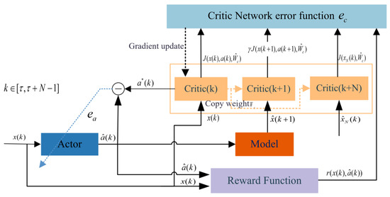
Figure 2.
The structure of the finite horizon reinforcement learning.
2.3.1. Action Network
The action network was adopted to approximate the control input . In this study, a fuzzy cerebellar model articulation controller (FCMAC) neural network was used as the approximator, providing a simple and fast approximator [30]. FCMAC requires fewer iterations and provides higher real-time accuracy than a BP network, making it suitable for the online learning problem in this study. The architecture of FCMAC includes input space, variable fuzzification, concept mapping, actual mapping and output space, as shown in Figure 3.
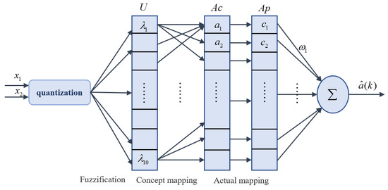
Figure 3.
The structure of the FCMAC.
The FCMAC network uses the fuzzification of the state quantity as the network input layer. The fuzzy variables based on the Gaussian membership function are as follows:
where is the centerpoint of the mth membership function, and are the variances. The middle layer of the FCMAC network includes two parts: concept mapping and actual mapping. Firstly, according to the fuzzification parameters, the space was divided into 10 storage units, which correspond to the fuzzy membership function vectors. Then, states were obtained by dividing the 10 fuzzy membership functions into fuzzy rules. Each state was mapped to the receptive field space C of Ac as a pointer associated with a storage unit, and the address corresponding to this state is found. Secondly, a division method used for false coding technology was adopted to map the elements C of the receptive field space to the units C in the physical memory space. This can be expressed as , where j stands for the unit after concept mapping. represents the remainder function in Matlab. represents the address of the concept mapping unit; represents the store address in the Ap. The output of FCMAC is expressed as:
where is the product of Gaussian membership function mapping and is the weight set. The objective of the action network is to minimize the error between the estimated value and the optimal value . The calculation of is described below. The error function is expressed as:
Then, the weight matrix updating rules for the action network are given by
where is the learning rate of the action network, which generally decreases to a fixed value with increasing time. C denotes the number of conceptual mapping storage cells. is the inertia coefficient of the action network.
2.3.2. Reward Function
The reward function serves as a training indicator to encourage or discourage actions. The target vehicle’s energy consumption on a road with traffic signal restrictions is shown in the study as a reinforcement learning environment, and the single-step reward function according to the eco-driving performance index of Equation (11) is expressed as follows:
In this study, the reward function in a finite horizon consisted of the terminal cost and cumulative return:
where is the terminal state for the current prediction horizon. is the terminal cost function, which is determined according to Formula (13). is discount factor, and .
2.3.3. Critic Network
Similar to the action network, the critic network adopted the FCMAC approximator. The output of the critic network based on FCMAC is expressed as:
where is the weight set and is the product of Gaussian membership function mapping. The estimated state was calculated according to the model, and the estimated value of the action network. can be estimated by through the critic network. According to and the reward function of Formula (18), Formula (19) is rewritten as
Based on the Bellman Optimality Equation, the optimal value function can be obtained as follows:
The optimal control law can be described by:
The optimal control strategy is vehicle acceleration in this study; that is, .
2.3.4. Critic Network Error Function
The function of the critic network error function is to modify the critic weight. This function was designed as the sum of the error considering the terminal constraint and cumulative return. According to Formula (21), the cumulative return error can be expressed as:
The terminal constraint network based on the FCMAC is represented as:
where is the product of Gaussian membership function mapping. is an estimated value of the terminal state, which is determined according to the initial state and the control law that is to be optimized. The terminal constraint error is expressed as
The ideal terminal constraint can be obtained from Formula (13). According to Formulas (24) and (26), the critic network error function is given by
The weight matrices update rules for the critic network are given by
where is the learning rate of the critic network. As also noted for the action network learning rate, this variable will gradually decrease to a fixed value. represents the Gaussian membership function of the critic network. is the inertia coefficient of the critic network.
According to the above method, a control sequence of length N was obtained, and the first () control actions were selected for implementation in the system. When was reached, the above methods were repeatedly used to solve the control problem. When arrived, the horizon advanced to . The system updated the prediction horizon length N, distance to traffic lights and vehicle status according to the V2X information, and the above method was repeated in the system. The main procedure of the proposed RHRL is summarized in Algorithm 1.
The solution method developed in this study is an online optimization control method that must satisfy real-time requirements. was used to set the maximum number of iterations in each finite horizon. When the iteration process reaches , the optimization process will be terminated, and the final optimized strategy will be applied to the system. To avoid unstable or bad strategies when the maximum number of iterations is reached, the initial weight value of each prediction horizon can be selected from the convex weight set in the previous prediction horizon. In this way, the learning time can be minimized, and control performance can be improved for real-time vehicle control.
| Algorithm 1 RHRL algorithm. |
The information on the upcoming road traffic light was obtained as well as the information on the vehicle. Then, the sampling time was set, and the length of the prediction horizon was estimated. The initialization of the vehicle state represents the initialization of parameters such as action network, critic network weights, learning rate, etc. The minimum error was set as and . The maximum number of iterations was set as and .
|
3. Lower-Level Multi-Objective Torque Control Allocation
The vehicle will deviate from the lane without intending to change lanes, as a result of the numerous unpredictable interferences encountered while maintaining the desired velocity (changes in the road, parameter perturbations, noise interference, etc.). In the lower controller, the vehicle must not only take fuel efficiency into account but also remain on the lane’s centerline and execute the necessary lateral stability control in unforeseen circumstances. Therefore, a multi-objective torque control allocation method that considers energy saving and safety was proposed in the lower-level control.
3.1. Vehicle 2-DoF Reference Model
The yaw rate and the slip angle are important parameters, used to describe the motion state of the vehicle. According to the 2-DOF model, the expected yaw rate is expressed as [31]:
where , and represent the distance from the center of mass to the front axle and rear axle. and denote the cornering stiffness values of the front and rear tires, is the steering angle of the front wheels. Based on the lateral dynamics, the lateral acceleration is . Meanwhile, the lateral acceleration is limited by the tire–road friction coefficient , as follows: . Then, the expected yaw rate can be expressed as:
The vehicle can achieve lateral stability control when the vehicle’s sideslip angle varies at around zero. In this paper, the desired sideslip angle was chosen to be so that fluctuates within a small range to ensure vehicle stability under critical conditions.
3.2. Torque Control Strategy
A 7-DOF model was employed in accordance with the dynamics and safety requirements of this study, since it provides more precise and quantitative dynamic equations and is closer to the actual vehicle. The seven degrees of freedom are longitudinal motion, lateral motion, yaw motion and the rotation of four wheels. The vehicle dynamics equation is expressed as:
where represents the front and rear track widths. It is assumed that is relatively small, such that , . The lateral forces on the front and rear wheels are expressed as:
The optimal distribution of driving/braking torque to each wheel ensures stable vehicle tracking while consuming less energy. The states of this control system were chosen as longitudinal speed, lateral speed and yaw rate of the vehicle, that is, ; the system control variables were selected for the four-wheel torque, that is ; the system output was chosen as . Substituting Equation (32) into Equation (31) yields
The dynamic model discussed above is a nonlinear system since the parameter f contains nonlinear elements. Nonlinear systems are challenging to solve and subpar real-time performance. Therefore, the Taylor series was used for approximate linearization in this study and, after discarding the high order, the following equation could be retained:
where and are the Jacobian matrix. represents the expansion point on the reference trajectory. We can obtain the linearised model as follows:
where . Discrete this linearized model; then, the equations can be written as follows:
where , , I is the unitary matrix. is the sampling time of the lower level. For the lower-level actuator, only short-term optimization needs to be completed; that is, the lower-level control only needs to solve the control solution at the next moment. Moreover, the sample time is also shorter than the upper-level control.
In this study, the state feedback method was used to solve the above problems. The state feedback control law is designed as follows:
The state feedback controller is designed to improve vehicle safety and economy, so the optimization objective function of this study was mainly composed of three parts, which are expressed as follows:
where are weight factors that can take on values from 0 to 1. The optimized objective function aimed to follow the velocity of the upper-level controller, yaw rate and slip angle to ensure stability.
where can be obtained from Section 3.1. The symmetric matrix can be adjusted according to the driving conditions.
The optimized objective function is the minimized tire utilization ratio, which reduces the sudden saturation of individual tire force and effectively improves the vehicle stability margin. This can be expressed as follows:
Since tire lateral force has little influence on the system and is uncontrollable, the control allocation presented here only considers the tire longitudinal force. Equation (39) can be simplified as:
The optimized objective function represents the minimization of energy consumption. For 4WIMD-EVs, the motor is the only power source. The influence of motor efficiency can be used to maximize the motor working in the high-efficiency region to achieve energy savings. The in-wheel motor power expression of the 4WIMD-EVs is shown as follows:
where is the motor speed. The change curve of motor efficiency obtained with the motor torque between 700 and 700 rpm is shown in Figure 4.
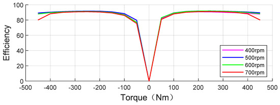
Figure 4.
Motor efficiency curve.
Substituting Equations (39), (41) and (43) into the objective function (38) can obtain the objective function
The state Equation (36) and the objective function (44) were used to establish the Hamiltonian function, and the expression is as follows:
where is a Lagrange multiplier vector. According to the Hamilton function, the control equation and covariance equation can be derived as
Using Equation (46a), the formulation of the control vector U can be derived as follows:
To facilitate the calculation of state feedback, the Lagrangian vector was defined according to optimal control theory as , where P and D are coefficient matrices. derivative was expressed as . Including and in the covariance Equation (46b). P was taken to be zero in a steady state and the covariance equation is collapsed to match the Riccati Equations (48) and (49), meaning that P was the result of Riccati Equation (48). The Riccati equation is represented as
According to Equation (48), P can be obtained. The Lagrange multiplier vector can be calculated using P and D, then added to Equation (47), and the feedback control law U is expressed as:
Through the above equation, the real-time display solution of the motor torque can be obtained. The vehicle reduces energy consumption while ensuring safety. Meanwhile, if one motor fails, the control algorithm can be reassigned by changing the G matrix in Equation (33) to achieve system reconstruction and effectively improve the vehicle’s stability in emergency situations.
4. Simulation and Analysis
The experimental platform included a driving simulator, a dSPACE for running control algorithms, a target machine for running a real-time vehicle model, a host for running a Carsim vehicle and control desk, and a SCANeR traffic scene host. The driver manipulated the steering wheel in the driving simulator to produce a certain steering wheel angle. The velocity planning module calculated the required torque according to the real-time traffic information and vehicle status transmitted via Ethernet. The steering wheel angle and torque signal were sent to the target machine at the same time, and the new position and state change of the vehicle was obtained. The result was sent to the traffic scene host and speed planning module via Ethernet, and the velocity planning module calculated the control torque according to the updated information. Thus, a closed loop was formed. The structure of the experimental platform is shown in Figure 5. The vehicle simulation parameters are shown in Table 1.

Figure 5.
Intelligent connected vehicle HIL experimental platform.

Table 1.
Parameters.
The initial speed of the adaptive cruise system was 60 km/h. The computer configuration used for the simulation was an Intel(R) Core(TM) i7-6700 CPU.
In the simulation, the maximum number of iterations in each RHRL time domain was = 50. The learning rates of the action network and the critic network were gradually reduced sequences ⋯ = 0.3, 0.25, 0.2⋯0.05. The iteration errors of the critic network and the actor network are shown in Figure 6a,b, and the cost function curve is shown in Figure 6c.
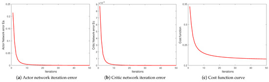
Figure 6.
The iteration errors and cost function curve.
In SCANeR, the simulation scenario was based on information about a certain section of the urban road and the time series of traffic lights. The experimental section was approximately 3.6 km, and there were five intersections. The control algorithm used in this study (RHRL), rule-based ACC algorithm (ACC) and predictive control algorithm (MPC) were tested using hardware-in-the-loop (HIL). The MPC algorithm adopted the interior point method to solve the problem in each prediction horizon. At the upper level, the sampling period was s.
Figure 7 and Figure 8 compare the strategies of the three algorithms regarding the distance domain and time domain, respectively. Compared with the ACC algorithm, the RHRL and MPC were based on the approaching intersection information, and the acceleration or deceleration of a vehicle was determined in advance. For example, MPC and RHRL accelerated the vehicle through the intersections based on advanced calculations according to the time remaining in a green phase at the 150–600 m section and 2100–2950 m section. However, ACC braked and stopped the vehicle at the traffic light. IN the MPC and RHRL control algorithms based on forward road information, the RHRL acceleration was relatively slow, which is more conducive to energy saving. At 1200 m, the vehicle using the three algorithms could not pass the intersection based on the time remaining at the traffic lights. MPC and RHRL adopted the method of idling at a permissible speed to reduce energy consumption. Figure 8 shows that the magnitude of ACC initiating mechanical braking was significantly higher than that of the MPC and RHRL algorithms at 45 s. For EVs, mechanical braking cannot regenerate energy. This means that the more mechanical brakes are activated, the more energy is consumed.
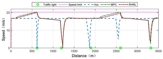
Figure 7.
The optimal and nominal speed planning results in the distance domain.
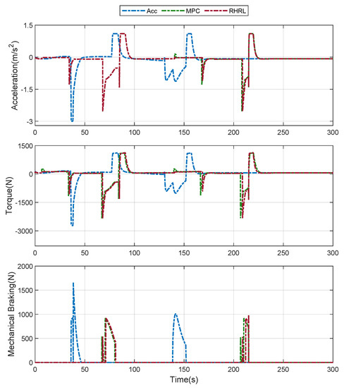
Figure 8.
Comparison of the results obtained following the proposed velocity trajectory planning, rule-based ACC and MPC at the upper level. From top to bottom, the figures show the trajectories of acceleration demand, torque demand and mechanical brake demand.
Compared with the rules-based ACC approach, the proposed algorithm and MPC accelerate and decelerate slowly in advance, considering the traffic information. Figure 9 shows the traffic light sequence and speed trajectory at multiple intersections. Meanwhile, the RHRL and MPC save overall driving time while reducing energy. In the acceleration stage, the acceleration of RHRL is relatively slow, which is more conducive to energy saving.
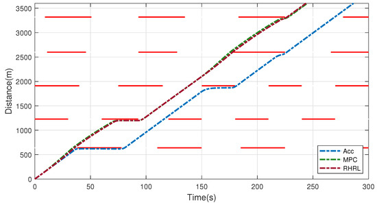
Figure 9.
The optimal and nominal trip time–distance results and traffic light schedules.
For computational efficiency, a receding horizon framework was adopted in this paper. In each prediction horizon, the complexity of the NMPC optimized by IPM is . The complexity of the method proposed in this paper is . Meanwhile, during the RHRL optimization process, the maximum number of iterations is set. When the total number of iterations is reached, the current strategy optimization is stopped and output is performed. This can be used to obtain suboptimal policies that balance computational efficiency and optimization effect. The computational time used in different prediction horizons is shown in Figure 10. The MPC algorithm increases the computational time with the increase in prediction horizon, which means that it is limited by the chip’s ability during engineering applications. However, the advantages of the RHRL algorithm in terms of computational performance become increasingly significant as the prediction horizon increases. As shown in Figure 10, when the prediction horizon length is 30, the calculation time of the MPC algorithm is about five times that of the RHRL algorithm. Therefore, the RHRL algorithm is more beneficial for engineering applications.
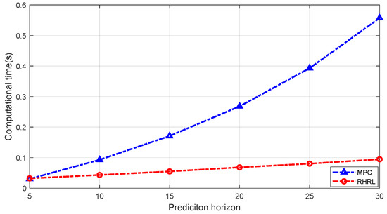
Figure 10.
Computational time at different prediction horizons.
According to the velocity tracking and lane-keeping requirements of the upper level, the multi-objective optimization results for the lower level are shown in Figure 11. For the lower-level executive motor, only short-term optimization needs to be completed according to the optimization velocity of the upper level. Then, the lower-level sampling period of the lower level selects . The combination of vehicle longitudinal acceleration and lateral lane change was selected for simulation validation of the algorithm, as shown in Figure 11.
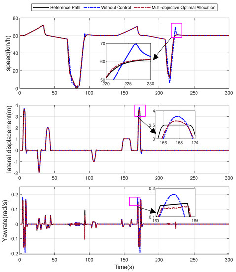
Figure 11.
Comparison of results following the proposed multi-objective torque allocation and torque equalization at the lower level. From top to bottom, the figure shows tracking control results for velocity, lateral displacement and yaw rate.
Without the control method, torque equalization occurs. The speed tracking curve shows that the error in the strategy without control significantly increases, and the upper-level demand eco-driving velocity cannot be tracked at 220–230 s. However, the multi-objective optimal allocation has a good tracking effect. From the lateral displacement and yaw rate tracking simulation diagrams, it can be seen that the strategy proposed in this study has a better control effect under acceleration and lane-changing conditions.
The torque allocation of the four motors is shown in Figure 12. The multi-objective optimal allocation method was used to adjust the motors to work in the high-efficiency area, effectively reducing the motor energy consumption. The two front motors always exert larger driving torques than the two rear motors, reducing the overall power consumption. Instantaneous power consumption is shown in Figure 13. The multi-objective optimal allocation method consumes less energy than the strategy without control.
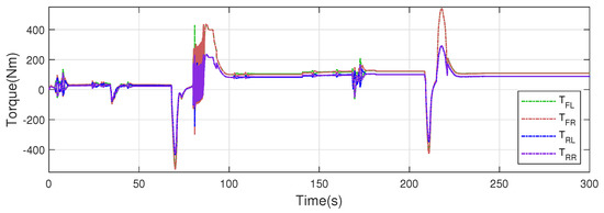
Figure 12.
Multi-objective optimal allocation for EVs.
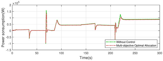
Figure 13.
Instantaneous power consumption.
Combined with the optimization algorithm of the upper and lower levels, the total energy consumption results for the three methods are shown in Figure 14, based on a simulated road of approximately 3.6 km in length with five traffic lights. The proposed approach saves approximately 12.98% energy consumption compared to the rule-based ACC algorithm.
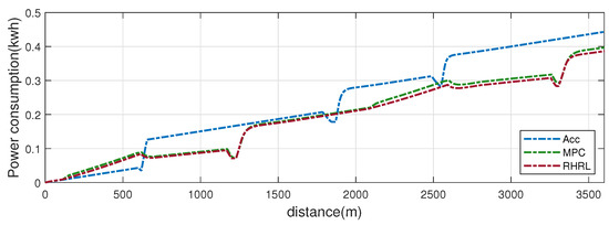
Figure 14.
Energy consumption in distance domain.
The simulation results demonstrate that the upper-level control strategy accelerates and idles immediately to prevent braking and restarting during the red light phase. Furthermore, it actually reduces energy consumption when combined with the lower-level multi-objective torque control allocation. Meanwhile, the strategy suggested in this study reduces traffic delays and increases traffic productivity.
5. Conclusions
In this study, based on an intelligent transportation system, an eco-driving cruise control strategy with a hierarchical structure for electric vehicles is proposed to rapidly optimize the velocity trajectories and torque control allocation display solution. The method minimizes energy consumption in an intelligent transportation system while ensuring safety.
- (1)
- The proposed RHRL method solves the computational time problem associated with long predictive horizons and high dimensionality in velocity planning and realizes the rapid solution of the energy-optimized cruising speed, thus improving the potential application of the controller in engineering practice.
- (2)
- A hierarchical control structure is used to optimize the energy at two levels, effectively reducing the complexity of the energy-efficient control of intelligent connected vehicles. The actuator comprehensively considers longitudinal velocity following and centerline lane-keeping, and a multi-objective optimal torque allocation method that considers energy saving and safety is proposed.
- (3)
- The control strategy is verified by building an intelligent connected HIL experimental platform for vehicles. Compared with ACC, the proposed approach reduces energy consumption by approximately 12.98%. In addition to the improved energy efficiency, the frequent accelerating and braking of vehicles is avoided, resulting in operating time and traffic efficiency benefits.
Author Contributions
Conceptualization, H.D. and K.G.; methodology, Z.Z. and N.Z.; software, Z.Z.; validation, Z.Z.; formal analysis, H.D. and N.Z.; data curation, Z.Z.; writing—original draft, Z.Z.; writing—review and editing, N.Z.; funding acquisition, H.D. and N.Z. All authors have read and agreed to the published version of the manuscript.
Funding
This research was funded by the China Automobile Industry Innovation and Development Joint Fund (grant No. U1864206); National Natural Science Foundation of China (grant 61790560); Niaona Zhang of the Science and technology development plan of Jilin province (grant number 20210201110GX) and the open fund of the State Key Laboratory of Automotive Simulation and Control (No. 20210237).
Informed Consent Statement
The study was conducted according to the guidelines of the Declaration of Helsinki and approved by the Institutional Review Board (or Ethics Committee) of the Changchun University of Technology.
Data Availability Statement
Not applicable.
Conflicts of Interest
The authors declare no conflict of interest.
References
- Neubauer, J.; Wood, E. The impact of range anxiety and home, workplace, and public charging infrastructure on simulated battery electric vehicle lifetime utility. J. Power Sources 2014, 257, 12–20. [Google Scholar] [CrossRef]
- Miao, Y.; Jian, C.L. An Eco-Driving Strategy for Partially Connected Automated Vehicles at a Signalized Intersection. IEEE Trans. Intell. Transp. Syst. 2022, 23, 15780–19753. [Google Scholar]
- Kamal, M.A.S.; Mukai, M.; Murata, J.; Kawabe, T. Ecological driver assistance system using model-based anticipation of vehicle-road-traffic information. Intell. Transp. Syst. 2011, 4, 244–251. [Google Scholar] [CrossRef]
- Bai, X.; Chen, G.; Li, W.; Zhu, A.; Wang, J. Critical Speeds of Electric Vehicles for Regenerative Braking. Automot. Innov. 2021, 4, 201–214. [Google Scholar] [CrossRef]
- Ubiergo, G.A.; Jin, W.-L. Mobility and environment improvement of signalized networks through Vehicle-to-Infrastructure (V2I) communications. Transp. Res. Part C Emerg. Technol. 2016, 68, 70–82. [Google Scholar] [CrossRef]
- He, H.; Liu, D.; Lu, X.; Xu, J. ECO Driving Control for Intelligent Electric Vehicle with Real-Time Energy. Electronics 2021, 10, 2613. [Google Scholar] [CrossRef]
- Asadi, B.; Vahidi, A. Predictive Cruise Control: Utilizing Upcoming Traffic Signal Information for Improving Fuel Economy and Reducing Trip Time. IEEE Trans. Control Syst. Technol. 2011, 19, 707–714. [Google Scholar] [CrossRef]
- Dib, W.; Chasse, A.; Moulin, P.; Sciarretta, A.; Corde, G. Optimal energy management for an electric vehicle in eco-driving applications. Control Eng. Pract. 2014, 29, 299–307. [Google Scholar] [CrossRef]
- Yang, H.; Rakha, H.; Ala, M.V. Eco-Cooperative Adaptive Cruise Control at Signalized Intersections Considering Queue Effects. IEEE Trans. Intell. Transp. Syst. 2016, 18, 1575–1585. [Google Scholar] [CrossRef]
- Zeng, X.; Wang, J. Globally energy-optimal speed planning for road vehicles on a given route. Transp. Res. Part C Emerg. Technol. 2018, 93, 148–160. [Google Scholar] [CrossRef]
- Nie, Z.; Farzaneh, H. Adaptive Cruise Control for Eco-Driving Based on Model Predictive Control Algorithm. Appl. Sci. 2020, 10, 5271. [Google Scholar] [CrossRef]
- Zhu, M.; Wang, Y.; Pu, Z.; Hu, J.; Wang, X.; Ke, R. Safe, efficient, and comfortable velocity control based on reinforcement learning for autonomous driving. Transp. Res. Part C Emerg. Technol. 2020, 117, 102662. [Google Scholar] [CrossRef]
- de Morais, G.A.P.; Marcos, L.B.; Bueno, J.N.A.D.; de Resende, N.F.; Terra, M.H.; Grassi, V., Jr. Vision-based robust control framework based on deep reinforcement learning applied to autonomous ground vehicles. Control Eng. Pract. 2020, 104, 104630. [Google Scholar] [CrossRef]
- Jia, Y.; Jibrin, R.; Itoh, Y.; Görges, D. Energy-Optimal Adaptive Cruise Control for Electric Vehicles in Both Time and Space Domain based on Model Predictive Control. IFAC-PapersOnLine 2019, 52, 13–20. [Google Scholar] [CrossRef]
- Guo, L.; Gao, B.; Gao, Y.; Chen, H. Optimal Energy Management for HEVs in Eco-Driving Applications Using Bi-Level MPC. IEEE Trans. Intell. Transp. Syst. 2017, 18, 2153–2162. [Google Scholar] [CrossRef]
- Guo, L.; Chen, H.; Liu, Q.; Gao, B. A Computationally Efficient and Hierarchical Control Strategy for Velocity Optimization of On-Road Vehicles. IEEE Trans. Syst. Man Cybern. Syst. 2018, 19, 31–41. [Google Scholar] [CrossRef]
- Bertsekas, D.P. Dynamic Programming and Suboptimal Control: A Survey from ADP to MPC. Eur. J. Control 2005, 11, 310–334. [Google Scholar] [CrossRef]
- Lin, Y.; McPhee, J.; Azad, N.L. Comparison of Deep Reinforcement Learning and Model Predictive Control for Adaptive Cruise Control. arXiv 2019, arXiv:1910.12047. [Google Scholar] [CrossRef]
- Zou, Y.; Guo, N.; Zhang, X.; Yin, X.; Zhou, L. Review of Torque Allocation Control for Distributed-drive Electric Vehicle. China J. Highw. Transp. 2021, 34, 1–25. [Google Scholar]
- Liu, W.; Khajepour, A.; He, H.; Wang, H.; Huang, Y. Integrated Torque Vectoring Control for a Three-Axle Electric Bus Based on Holistic Cornering Control Method. IEEE Trans. Veh. Technol. 2018, 67, 2921–2933. [Google Scholar] [CrossRef]
- Zhai, L.; Sun, T.; Jie, W. Electronic Stability Control Based on Motor Driving and Braking Torque Distribution for a Four In-Wheel Motor Drive Electric Vehicle. IEEE Trans. Veh. Technol. 2016, 65, 4726–4739. [Google Scholar] [CrossRef]
- Liu, R.; Wei, M.; Sang, N.; Wei, J. Research on Curved Path Tracking Control for Four-Wheel Steering Vehicle considering Road Adhesion Coefficient. Math. Probl. Eng. 2020, 2020, 3108589. [Google Scholar] [CrossRef]
- Zhang, X.; Göhlich, D.; Zheng, W. Karush–Kuhn–Tuckert Based Global Optimization Algorithm Design for Solving Stability Torque Allocation of Distributed Drive Electric Vehicles. J. Frankl. Inst. 2017, 354, 8134–8155. [Google Scholar] [CrossRef]
- Jalali, M.; Khajepour, A.; Chen, S.; Litkouhi, B. Integrated stability and traction control for electric vehicles using model predictive control. Control Eng. Pract. 2016, 54, 256–266. [Google Scholar] [CrossRef]
- Gao, B.; Yan, Y.; Chu, H.; Xu, N. Torque allocation of four-wheel drive EVs considering tire slip energy. Sci. China Inf. Sci. 2022, 65, 122202. [Google Scholar] [CrossRef]
- Peng, H.; Wang, W.; Xiang, C.; Li, L.; Wang, X. Torque Coordinated Control of Four In-Wheel Motor Independent-Drive Vehicles with Consideration of the Safety and Economy. IEEE Trans. Veh. Technol. 2019, 68, 9604–9618. [Google Scholar] [CrossRef]
- Guo, N.; Zhang, X.; Zou, Y.; Lenzo, B.; Du, G.; Zhang, T. A Supervisory Control Strategy of Distributed Drive Electric Vehicles for Coordinating Handling Lateral Stability, and Energy Efficiency. IEEE Trans. Transp. Electrif. 2021, 99, 2488–2504. [Google Scholar] [CrossRef]
- Wei, H.; Ai, Q.; Zhao, W.; Zhang, Y. Modelling and experimental validation of an EV torque distribution strategy towards active safety and energy efficiency. Energy 2022, 239, 121953. [Google Scholar] [CrossRef]
- Dong, H.; Zhuang, W.; Chen, B.; Yin, G.; Wang, Y. Enhanced Eco-Approach Control of Connected Electric Vehicles at Signalized Intersection with Queue Discharge Prediction. IEEE Trans. Veh. Technol. 2021, 70, 5457–5468. [Google Scholar] [CrossRef]
- Guan, J. Research on Adaptive Control Based on CMAC for Nonlinear Systems; Xiamen University: Xiamen, China, 2019. [Google Scholar]
- Ma, Y.; Chen, J.; Zhu, X.; Xu, Y. Lateral stability integrated with energy efficiency control for electric vehicles. Mech. Syst. Signal Process. 2019, 127, 1–15. [Google Scholar] [CrossRef]
Disclaimer/Publisher’s Note: The statements, opinions and data contained in all publications are solely those of the individual author(s) and contributor(s) and not of MDPI and/or the editor(s). MDPI and/or the editor(s) disclaim responsibility for any injury to people or property resulting from any ideas, methods, instructions or products referred to in the content. |
© 2023 by the authors. Licensee MDPI, Basel, Switzerland. This article is an open access article distributed under the terms and conditions of the Creative Commons Attribution (CC BY) license (https://creativecommons.org/licenses/by/4.0/).