Research on Rolling Bearing Fault Diagnosis Based on Variational Modal Decomposition Parameter Optimization and an Improved Support Vector Machine

Abstract

Aiming at the problems of modal aliasing and poor noise resistance when processing the vibration acceleration signal of rolling bearings by empirical modal decomposition (EMD), a variational modal decomposition (VMD) method based on parameter optimization is proposed. Combined with the improved particle swarm optimization algorithm (IPSO) and improved envelope entropy, the VMD decomposition layers and penalty parameters were optimized. The components with high correlation coefficients with the original signal were screened out, and the fault characteristics were extracted by combining the sample entropy. Aiming at the low classification accuracy of the support vector machine with fixed parameters in the fault diagnosis stage and the defects of the gray wolf algorithm, such as insufficient population diversity and large influence of the initial population on the optimization effect, an improved gray wolf algorithm (IGWO) based on multistrategy improvement is proposed. The IGWO was combined with the support vector machine to obtain an improved gray wolf algorithm optimization support vector machine (IGWO-SVM). The rolling bearing fault diagnosis test bench is established to collect the vibration acceleration signals of rolling bearing under different states. The experimental results show that the fault diagnosis of rolling bearings with strong noise can be effectively realized by applying the above methods, and the average fault diagnosis accuracy rate reaches 98.875%.

1. Introduction

The driving motor of an electric vehicle is the main source of its power. In addition, the rolling bearing is the core component of the driving motor. Its safety is the key to affecting the reliability and safety of the whole vehicle. Studying the fault diagnosis method of rolling bearings and improving the accuracy of fault diagnosis can reduce the probability of electric vehicle traffic accidents and improve the safety level. In light of the nonstationary characteristics of the rolling bearings in electric vehicles, the fault signals are complicated and have many interference factors. Scholars have developed a variety of methods to analyze and process the vibration acceleration signal of rolling bearings to extract effective fault features, such as EMD, EEMD, LMD, etc. [1,2,3,4]. However, these methods have problems, including modal aliasing and endpoint effects, until Dragomiretskiy et al. [5] proposed the variational mode decomposition (VMD) method, which had a solid theoretical foundation and effectively solved the defects mentioned above. So, scholars have begun to try to use the VMD method to solve the fault diagnosis problem of rolling bearings.

Liu et al. [6] determined the number of VMD decomposition layers K by observing the central frequency of the VMD component combined with the fuzzy mean clustering method to realize the fault diagnosis of rolling bearings. Wang et al. [7] determined the number of VMD decomposition layers K based on the ratio between the component energy and the total energy of the original signal. Li et al. [8] combined the information entropy algorithm to optimize the number of decomposition layers K of VMD. Zhang et al. [9] used an artificial fish swarm algorithm combined with envelope entropy to optimize the number of VMD decomposition layers K and achieved good results. Chang et al. [10] used the correlation coefficient between components and the original signal to optimize the number of decomposition layers of VMD. Zhu et al. [11] used the swarm algorithm to optimize the VMD parameters using the steepness as an index, and Zhang et al. [12] used the particle swarm optimization (PSO) algorithm with gradient information to optimize the number of VMD decomposition layers. From the research results of past scholars, it is not difficult to find that the difficulty of using the VMD method lies in the selection of the VMD parameters. However, most scholars pay attention to the influence of the number of VMD decomposition layers K on the decomposition effect in isolation and ignore the influence of the combination of the number of decomposition layers K and the penalty parameter α. In addition, some scholars often determine the number of decomposition layers K by increasing or decreasing the layer number, which is inefficient.

After using signal processing technology to realize a multiscale analysis of bearing vibration signals and using appropriate feature extraction technology to extract the characteristics of bearing vibration signal failures, it is also necessary to accurately identify the fault type and fault location of the bearing. Hao et al. [13] used the vibration signal as the input of the convolutional neural network to realize the fault diagnosis; Deng et al. [14] used a convolutional neural network (CNN) for rolling bearing fault diagnosis; Chen et al. [15] used a CNN model with an attention guidance mechanism to realize the fault characteristics of rolling bearings; Pinedo et al. [16] used a CNN network to analyze the bearing vibration signal, and the fault diagnosis effect was good. Although rolling bearing fault diagnosis using artificial neural networks is good, this method requires a large number of samples to train the neural network to ensure the final fault diagnosis effect. In contrast, support vector machines classify better with small samples. Song et al. [17] used the global sparrow search algorithm to optimize the parameters of the SVM, and Meng et al. [18] used the PSO algorithm to optimize the parameters of the least squares SVM (LS-SVM). Chen et al. [19] combined chaos mapping with a bat algorithm to optimize the kernel parameters of the support vector machine. Ma et al. [20] used the sparrow search algorithm to optimize the penalty parameters and kernel parameters of the support vector machine. Although many scholars have conducted a lot of research, the parameter selection of a support vector machine is still a difficult problem, and there is no unified determination method. The gray wolf algorithm (GWO) is a swarm intelligence algorithm based on the hunting process of gray wolves. More and more scholars are paying attention to this intelligent search algorithm and applying it to many fields. Zhou et al. [21] used the gray wolf algorithm to optimize the support vector machine to predict the seismic trend, Cui et al. [22] optimized the product-based neural network (PNN) with the gray wolf algorithm, Sharma et al. [23] optimized the routing process of the Internet of Things with the gray wolf algorithm, Faiza et al. [24] used the GWO to plan the robot path, and Ma et al. [25] used the GWO to optimize the parameters of the extreme learning machine to evaluate beam performance. However, the GWO has the shortcomings of difficulty in balancing global optimization and local search in the iterative process, poor global search ability, the large impact of the quality of the initial population on the efficiency of the algorithm, and insufficient population diversity.

This article is mainly divided into five parts. After the introduction, it mainly discusses the method of optimizing VMD parameters based on an improved particle swarm optimization algorithm (IPSO). VMD requires optimal parameters, including the number of decomposition layers and penalty parameters. The one-way row of information exchange between the individual particles of the particle swarm algorithm allows the neighborhood operator not to destroy the better values already searched for. In terms of convergence, the particle swarm algorithm is superior and more suitable for the task of tuning VMD parameters. In the third part, the optimization of kernel function parameters and penalty parameters of support vector machines using the improved gray wolf algorithm (IGWO) is performed for rolling bearing fault diagnosis using parameter-optimized SVM. The fourth part is the experimental part. Under laboratory conditions, the vibration acceleration signal of different fault types of rolling bearing is collected based on the rolling bearing fault test bench. In addition, IPSO-VMD combined with an IGWO-SVM is used to diagnose the fault of rolling bearings with the collected data. Then, the fault diagnosis results are compared and analyzed with multiple methods. The last part summarized all the research contents and puts forward the follow-up work.

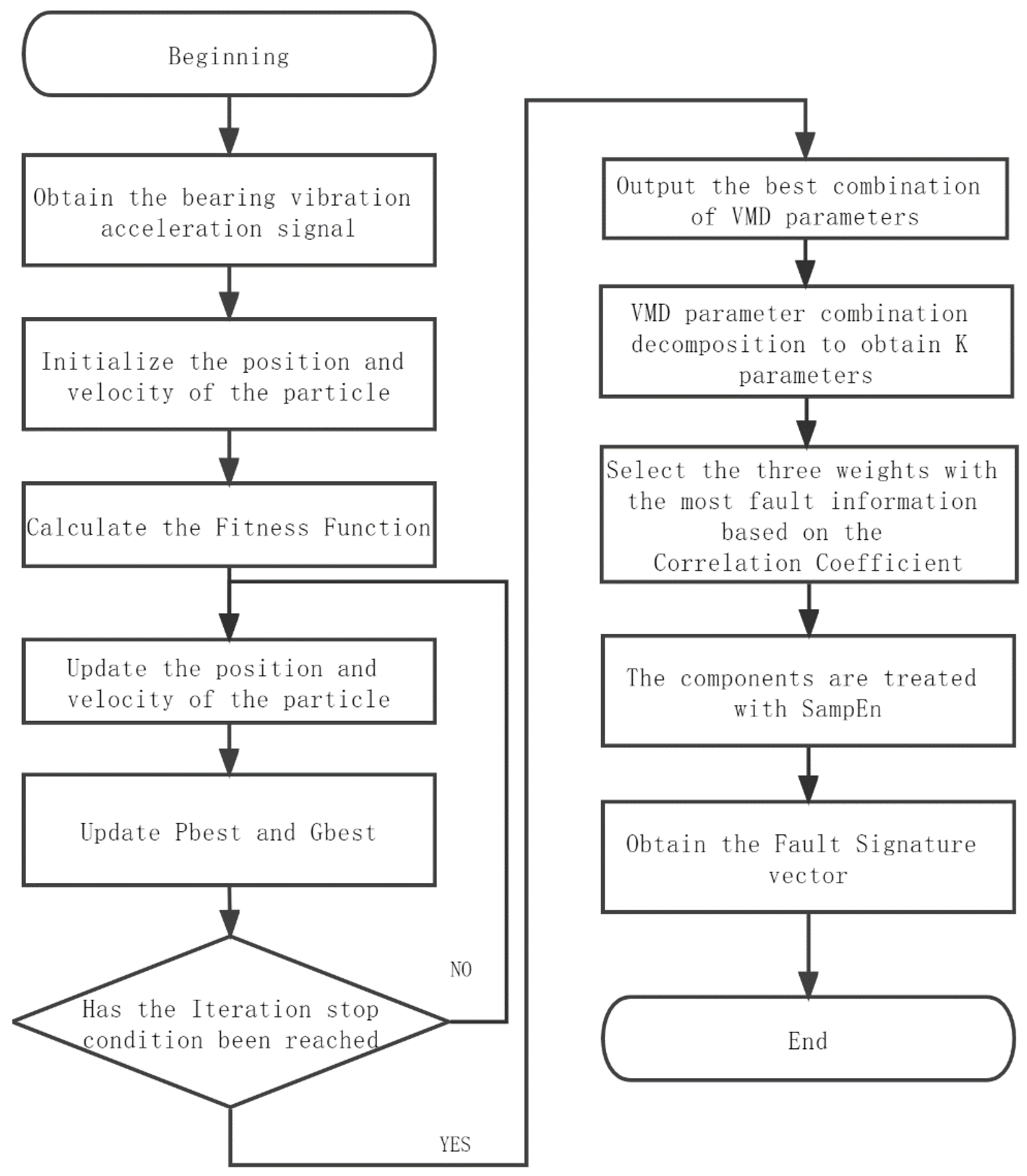
2. Fault Feature Extraction Algorithm for Rolling Bearings Based on IPSO-VMD

Firstly, when VMD is used to process signals, it is difficult to select the appropriate number of decomposition layers and penalty parameters. Accordingly, the improved particle swarm optimization algorithm (IPSO) combined with the improved envelope entropy algorithm was used to comprehensively analyze and determine the two important parameters, which lays a foundation for subsequent fault diagnosis.

2.1. Principle of Variational Modal Decomposition

The first step in VMD is to transform the signal decomposition problem into a variational problem. To ensure that the original signal, after the variational modal decomposition, becomes a certain number of modal components with a certain bandwidth and respective center frequency, Equation (1) was constructed. All the modal components obtained after the decomposition were added up to obtain the original signal, which was used to be the constraint of the constructed variational problem to obtain the minimum value of the sum of the bandwidths of all the modalities.

$$\underset{u_k,{\omega }_k}{\mathit{min}}\left\{{\displaystyle \sum }_k\Vert {\partial }_t\left[(\delta \left(t\right)+\frac{j}{\pi t})\ast u_k\left(t\right)\right]e^{-2\pi j{f}_{k}t}{\Vert }_2^2\right\}$$

(1)

$$s.t.{\displaystyle \sum }_{k=1}^k{u}_k=f\left(t\right)$$

(2)

where * represents the convolution operation, ${\partial }_t$ represents the gradient calculation, $\delta \left(t\right)$ is the unit pulse,$f_k$ is the component center frequency, $u_k$ is each component whose expression is $u_k\left(t\right)=A_k\left(t\right)\cos \left({\varphi }_k\left(t\right)\right)$, and ${\varphi }_k\left(t\right)$ represents the phase of the modal components, and it is a nondecreasing function, ${{\varphi }_k}^{\prime }\left(t\right)⩾0$; if the envelope is non-negative, then $A_k\left(t\right)⩾0$.

The augmented Lagrangian expression is constructed using the Lagrangian multiplication operator and the quadratic penalty factor. By obtaining the corresponding optimal solution, the original signal can be decomposed into K components with determined center frequency and bandwidth.

2.2. Improved Particle Swarm Optimization Algorithm

The particle swarm optimization (PSO) algorithm assumes that there is a population with N particles in a given solution space. Velocity and position are the parameters of particles where the velocity information represents the direction of motion, and the position information represents the solution to be optimized in the problem. The iterative formula is used to continuously iterate the parameters. As the population continues to iterate, the particle position gradually approaches the global optimal position. As a result, the global optimal solution is obtained. The velocity iteration process for each particle is shown in Equation (3).

$$v_i^{k+1}=h{v}_i^k+c_{1}r\left(p_i^k-x_i^k\right)+c_{2}r\left(g_i^k-x_i^k\right)$$

(3)

where $v_i^{k+1}$represents the velocity of the i-th particle in the particle swarm at the (k + 1)st iteration, $v_i^k$ represents the velocity of the i-th particle at the k-th iteration, $x_i^k$represents the position of the i-th particle at the k-th iteration, and $h$ represents the inertia weight, which makes the PSO algorithm iterate in such a way that each generation of particles inherits the characteristics of the previous generation of particles. $c_1$ and $c_2$ represent the learning factors, and r is a random number whose range is from 0 to 1.$p_i^k$ represents the extreme individual value of the i-th particle at the k-th iteration, and the individual extreme is the value of the current particle that has the best fitness among all previous iterations. $g_i^k$ represents the best-adapted value of all particles in the whole particle population and is called the global extreme value.

Through the study of the standard PSO algorithm, it can be found that the inertia weight coefficient determines the inheritance of the previous generation of particle characteristics during iteration, which gives each particle the ability to search the solution space during iteration [26]. The global search ability is strengthened with the increase of the inertia weight coefficient, but the local search ability is inversely proportional to the inertia weight coefficient. The parameters are fixed values in the standard PSO, which causes precociousness and stagnation of the algorithm. So, the IPSO is expected to be obtained.

(1)

Set the inertia weight coefficient based on the random strategy

In the adaptive improvement of VMD using PSO, it is required to have a superior global search capability and diversity of particle populations. Given this, the equation of the random inertia weight coefficient shown in Equation (4) is constructed based on the random strategy.

$$v=u_{\mathit{min}}+(u_{\mathit{max}}-u_{\min })\times rand$$

(4)

where $v$ represents the inertia weight coefficient, $u_{\mathit{min}}$ represents the minimum inertia weight coefficient value, $u_{\mathit{max}}$ represents the maximum inertia weight coefficient, and rand represents a random number between (0,1). The inertia weight is directly proportional to the global searchability of the algorithm, setting the minimum and maximum values of the inertia weights to be 0.9 and 1.2, respectively [27]. Random inertia weights based on stochastic policies enable the algorithm to coordinate global and local searches more flexibly during iterations.

The random inertia weight coefficient can result in a large or small inertia weight coefficient in the early and later stages. In the process of particle iteration, when the particle population is far from the optimal solution, the larger inertia weight helps to strengthen the global optimization ability. When the particle population is near the optimal solution, the small inertial weight brings about a local fine search, which helps to strengthen the local optimization ability. Compared with the fixed inertia weight coefficient, the inertia weight coefficient based on the random strategy can make the overall and local optimization of the IPSO more flexible and will not cause algorithm stagnation when the appropriate inertia weight is not set at the beginning.

(2)

Setting learning factors based on linearly varying policies

The iterative formula of standard PSO contains two learning factors, $c_1$ and $c_2$. The selection of these two factors has a great influence on the operation of PSO.$c_1$ is called the individual learning factor and represents the degree of influence of each individual’s historical optimal solution on that individual. $c_2$ is called the social learning factor and represents the influence of the optimal solution on each individual in the entire population.

To better optimize the VMD parameter combination, the optimal solution of individuals should be paid more attention in the early stage. The optimal global solution should be paid more attention in the latter stage. Therefore, this paper uses a linear change strategy to improve the learning factor, which will change linearly with the iteration finally. The two learning factors are iterated using Equations (5) and (6).

$$c_1=c_{1max}+\left(c_{1min}-c_{1max}\right)\times \frac{t}{T_{max}}$$

(5)

$$c_2=c_{2max}+\left(c_{2max}-c_{2min}\right)\times \frac{t}{T_{max}}$$

(6)

where $c_{1min}$ is the minimum value of individual learning factors, and $c_{1max}$ is the minimum value. They are taken as 1.5 and 2, respectively. $c_{2min}$ and $c_{2max}$ are the minimum and maximum values of the social learning factors, which are taken as 1.5 and 2, respectively.

2.3. Fitness Function

The selection of penalty parameters and decomposition layers during the implementation of the VMD method has a great influence on the decomposition effect. So, IPSO is used to optimize the VMD parameters. A suitable fitness function is also required. In this paper, an improved envelope entropy combined with envelope steepness is used as a fitness function, and the expression of envelope entropy is shown in Equations (7) and (8).

$$H\left(x\right)=-{\displaystyle \sum }_{i=1}^{N}p\left(i\right)lgp\left(i\right)$$

(7)

$$p\left(i\right)=\frac{H_b\left(i\right)}{{{\displaystyle \sum }}_{i=1}^N{H}_b\left(i\right)}$$

(8)

where $H\left(x\right)$ represents the envelope entropy of a continuous time series x, and $H_b\left(i\right)$ represents the envelope signal.

However, the envelope entropy cannot show the impact of the bearing signal, but the steepness index is very sensitive to the impact component. The more obvious the impact component is, the greater the value of the steepness index will be. The steepness of the component envelope is calculated as shown in Equation (9).

$$K_r=\frac{N{{\displaystyle \sum }}_{i=1}^N{\left(x_i-\tilde{x}\right)}^4}{{({{\displaystyle \sum }}_{i=1}^N{\left(x_i-\tilde{x}\right)}^2)}^2}$$

(9)

where N is the sample number of the envelope signal, $x_{i }$ is each sample of the envelope, and $\tilde{x}$ is the average of all samples.

Combining the envelope entropy algorithm and envelope steepness index, the improved envelope entropy is obtained, which is labeled as $E_{KH}$, as shown in Equation (10).

$$E_{KH}=\frac{H}{K_r}$$

(10)

where $K_{r }$ is the cliff, and $H$ is the envelope entropy.

After variational modal decomposition, the obtained modal components will contain fault information. The better the decomposition effect is, the more fault information can be contained in the components, and the more obvious the periodic fault impact signal will be. Accordingly, the periodicity of the signal will be stronger, the envelope entropy of the components will be smaller, and the envelope cliff value will be greater. The new envelope entropy value $E_{KH}$ can be obtained by dividing the minimum H of each decomposition by the maximum $K_{r }$, which is the fitness function of the IPSO, so that the periodicity and impact of the components can be taken into account when finding the optimal VMD decomposition parameters. Finally, the optimal number of decomposition layers and the penalty parameters corresponding to them can be found.

2.4. Fault Feature Extraction and Testing

After optimization of the VMD parameters by the IPSO, the complexity of each component varies. Therefore, in this paper, the sample entropy is selected as the fault feature used for rolling bearing fault diagnosis. A combination of parameter-optimized variational modal decomposition and sample entropy is used to extract the fault feature vectors of the bearings. The flowchart is shown in Figure 1. The specific steps are as follows:

Step 1: the improved particle swarm algorithm is used to analyze the original vibration signal, determine the number of decomposition layers and penalty parameters, and decompose the variational mode of the vibration signal to obtain K components.

Step 2: Select the three components with the most fault information based on the correlation coefficient of the VMD component and the original signal.

Step 3: Determine the embedding dimension m and the similar tolerance threshold r of the sample entropy algorithm. The selection of the embedding dimension m and the tolerance threshold r will have some impact on the calculation results of the sample entropy in the time series. The embedding dimension of the sample entropy was set to 2, and the similarity tolerance threshold was 0.2 times the standard deviation of the sequence [28].

Step 4: The sample entropy algorithm is used to process the three selected components separately. Take the results as a fault feature vector and construct a fault feature vector group that can be used for bearing fault diagnosis.

The performance analysis experiment was based on the public-bearing experimental data of Western Reserve University. The bearing used in the experiment of Western Reserve University was a 6205-RS deep groove ball bearing, which had an outer ring diameter of 52 mm and an inner ring diameter of 25 mm, a rolling element segment diameter of 35 mm, and a width of 15 mm. The bearing speed was 1750 r/min. The sampling frequency was 12 KHz [27]. The bearing experimental signal of the outer ring fault was analyzed. The fault point width was 0.1778 mm. A total of 4096 sampling points were selected for analysis. The fault characteristic frequency is 104.6 Hz in theory. When the outer ring of the bearing fails, the time domain waveform diagram is shown in Figure 2. The signal has obvious periodic shocks.

To get closer to the noise environment that rolling bearings face in a real environment, an additional noise signal was added to the signal. Noise with an intensity of −8 dB was added, and the time domain diagram of the signal with strong noise is shown in Figure 3.

It can be found that the periodic shock components have been completely covered by noise, and the state of the bearing cannot be judged directly. The envelope spectrum was analyzed for the signal containing strong noise, and the envelope spectrum is shown in Figure 4.

Obviously, the noise has a serious impact on the signal envelope spectrum. There are no obvious frequency components in the figure. The fault frequency cannot be found. This shows that the traditional envelope spectrum analysis method based on fault characteristic frequency cannot effectively realize fault diagnosis.

The VMD parameters of the vibration signal with outer ring failure were optimized using the IPSO-VMD method. The iterative diagram of the fitness function is shown in Figure 5.

When the algorithm iterated to the sixth generation, the corresponding fitness value was the minimum of 0.02925. At this time, the corresponding VMD parameter combination [number of decomposition layers, penalty parameter] was [12, 8219]. Using this parameter combination to decompose the vibration signal, 12 components were obtained. Component 8 has the highest correlation coefficient with the original signal. Envelope spectrum analysis was performed on it. As shown in Figure 6, there was an obvious peak at the fault characteristic frequency of 105.5 Hz. The fault location can be judged. At the same time, the noise component of the signal is also very low, which shows the superior antinoise performance of the IPSO-VMD method.

To further compare the performance of the algorithms, the fixed-parameter VMD method and the EMD method with three decomposition layers and a penalty parameter of 500 were used to decompose the noise-containing signal and to perform envelope spectrum analysis on the components. Respectively, the envelope spectrum of the fixed-parameter VMD component containing the most fault information is shown in Figure 7, and the envelope spectrum of the best EMD component is shown in Figure 8.

The envelope spectrum of the best EMD component has many noise components in Figure 8, and the peak of fault frequency is not prominent. So, it is difficult to determine the bearing fault type by the fault characteristic frequency. On the contrary, the fault characteristic frequency in Figure 7 is clearer and more prominent than that in Figure 8. However, compared with the envelope spectrum in Figure 6, it can be found that the IPSO-VMD method has stronger antinoise performance and a stronger ability to decompose fault information and extract fault characteristics from the fixed-parameter VMD and EMD methods.

The signal was reconstructed by the first three components with the largest correlation coefficient. The signal-to-noise ratio and mean square error between the reconstructed signal and the original signal were calculated, respectively. The results are shown in

Table 1. Comparison of different methods.

Signal Type	Signal-to-Noise Ratio (SNR)	Mean Square Error (MSE)
Noisy Signal	−8	2.0394
EMD	−7.6971	1.8701
Fixed parameter VMD	−5.8897	1.4549
IPSO-VMD	1.0934	0.2471

. Comparing the three methods, it can be found that the reconstructed signal obtained by using the IPSO-VMD method has the highest signal-to-noise ratio value and the lowest mean square error, indicating that the IPSO-VMD method has a better decomposition effect compared with the traditional EMD method and the VMD method with fixed parameters. Therefore, it is more suitable for the decomposition of a rolling bearing vibration acceleration signal with strong noise interference.

3. Bearing Fault Diagnosis Based on IGWO-SVM

In order to apply SVM to rolling bearing fault diagnosis, the kernel function parameters and penalty parameters need to be determined in advance, which has a great influence on the classification effect. Therefore, these parameters were optimized by using the improved gray wolf algorithm (IGWO).

3.1. Principle of Support Vector Machine

The SVM is a supervised classification model based on statistical learning theory and the structural risk minimization principle. Compared with other classification algorithms, the advantage of the SVM is the superior classification effect of small samples. The SVM is able to achieve high classification accuracy with small training sample sizes. Since the bearings are in normal operation most of the time in actual operation, the number of various fault state data is not rich, so this paper selected the support vector machine for the classification of rolling bearing faults.

The linear equation for the hyperplane is shown in Equation (11). Among them, $w$ is the normal vector, and $b$ is the displacement amount.

$$w^{T}x+b=0$$

(11)

Assuming that the hyperplane can correctly classify the training samples, for the sample points $(x_i,y_i)$ satisfied, the sample point closest to the hyperplane such that the inequality equation can hold is called the support vector.

$$\{\begin{array}{l}{w}^T{x}_i+b\ge +1,y=+1\\ w^T{x}_i+b\le -1,y=-1\end{array}$$

(12)

To maximize the classification ability of the SVM, it is required to maximize the distance from the support vector to the hyperplane. Thus, maximizing the interval problem is the process of solving the convex quadratic programming, as shown in Equation (13). This is the basic type of support vector machine.

$$\{\begin{array}{l}\underset{w,b}{\mathit{min}}\frac{1}{2}{\Vert w\Vert }^2\\ \begin{array}{cc}s.t.& y_i(w^T{x}_i+b)\ge 1\end{array},i=1,2,\cdots ,n\end{array}$$

(13)

The Lagrangian multiplier method is introduced to construct the Lagrangian function as shown in Equation (14).

$$L(w,b,\alpha )=\frac{1}{2}{\Vert w\Vert }^2-{\displaystyle \sum _{i=1}^n{\alpha }_i[y_i(w^T{x}_i+b)-1]}$$

(14)

Among them, $\alpha$ is the Lagrangian coefficient and not negative. Finding the minimum value of Equation (14), we find partial differentiation for w and b, respectively, and make it equal to 0. Then, the interval problem turns into a dual problem.

For the linearly inseparable case, it is necessary to modify the constraints of Equation (13) as well as the objective function. To add a relaxation variable ${\xi }_i$ and a penalty factor $C$, as shown in Equation (15), the relaxation factor allows the existence of outliers to be allowed, and the penalty factor represents the degree of tolerance for outliers, and the penalty factor has a significant impact on SVM classification.

$$\{\begin{array}{l}\min \frac{1}{2}{\Vert w\Vert }^2+C{\displaystyle \sum _{i=1}^n{\xi }_i}\\ \begin{array}{cc}s.t.& y_i(w^T{x}_i+b)\ge 1\end{array}-{\xi }_i,i=1,2,\cdots ,n\end{array}$$

(15)

When facing the problem of nonlinear classification, the radial basis kernel function needs to be introduced to map the original data to the high-dimensional space by the nonlinear mapping method and then an optimal classification plane in the high-dimensional space must be found. The radial basis kernel function is better for small sample classification problems than for other kernel functions. When the radial basis kernel function is used as an SVM kernel function, the parameters that most affect the classification effect of SVM are the penalty factor $C$ and the kernel function parameter g.

3.2. Improved Gray Wolf Algorithm

The nonlinearly decreasing distance parameter strategy and the population initialization strategy are introduced into the GWO. Then, the differential evolution algorithm is used, so as to increase population diversity, prevent the algorithm from maturing early and falling into the local minimum, improve the global search performance, and enhance the search efficiency.

(1)

Distance parameter strategy based on nonlinear control

The distance parameter of the GWO controls the global search and local search during the iteration process. With the linear decrease of the distance parameter, the advantage in local search is gradually enhanced, while the overall searchability is decreasing. Therefore, due to the over quick deceleration of the distance parameter in the early stage, it is easy to miss the global optimal solution and enter the local search stage early. Aiming at this shortcoming, referring to the nonlinear inertia weight of PSO [29], the following nonlinear decreasing distance parameter strategy is proposed, as shown in Equation (16).

$$a=\left(a_1-a_2\right)·{[(e^{t/t_{max}}-1)/\left(e-1\right)]}^2$$

(16)

where $a$ represents the distance parameter, $a_1$ represents the initial value of the distance parameter, $a_2$ represents the final value of the distance parameter, $t$ represents the current iteration number, and $t_{max}$ represents the maximum iteration number.

The nonlinearly decreasing distance parameter varies with each iteration, as shown in Figure 9. The nonlinear decreasing distance parameter decays slowly in the early stage, which keeps the GWO in the global search state for a long time, which is of great help to enhance the global optimization performance. In the later stage, the attenuation speed of the distance parameter is accelerated, which can speed up the convergence and strengthen the local search ability.

(2)

Population initialization strategy based on the good-point set theory

The initial population of the standard GWO is obtained randomly. It is easy to be unevenly distributed in the solution space and for some individuals to aggregate, resulting in premature maturity and convergence of the algorithm, and finally falling into the local optimal value.

This paper establishes a gray wolf population initialization strategy based on the good-point set theory. Suppose that in a d-dimensional Euclidean space, the set of good points is defined as shown in Equation (17).

$$p_n\left(k\right)=\left\{\left(\left\{r_1\ast k\right\},\left\{r_2\ast k\right\}\cdots \left\{r_d\ast k\right\}\right),1\le k\le n\right\}$$

(17)

where $r$ is the good point, and n is the point number [30]. Under the condition that the population number is consistent, the individual distribution of the initial population obtained by the initialization strategy based on the good-point set theory is more uniform. There is no individual aggregation or overlap, and the population quality is much better than the random initial population.

(3)

Population diversification strategy based on mutation crossover

The differential evolution algorithm (DE) is a group intelligence algorithm that obtains the optimal direction based on the collaboration between individuals in a population. The mutation strategy is to randomly select three different individuals from the population, make differences between two of them, and fuse the obtained difference vector with another body to obtain a variant, the specific process of which is shown in Equation (18).

$$D_i\left(t+1\right)=X_1\left(t\right)+F\left(X_2\left(t\right)-X_3\left(t\right)\right)$$

(18)

where $t$ represents the iterations number, $D_i$ is the mutant individual, and F is the scaling factor, which is generally set to some number between 0 and 1.

Cross-operation is performed to exchange some elements of the original individual with some elements of the mutated individual, so as to obtain a new individual to increase population diversity. For the j-dimensional element of the ith individual, the cross-operation process is shown in Equation (19).

$$U_{ij}\left(t+1\right)=\{\begin{array}{c} D_{i,j}\left(t+1\right)rand<C or j=S\\ X_{i,j}\left(t\right)\end{array}$$

(19)

where $C$is the cross probability, $rand$ represents a random number between 0 and 1, and $S$ is a random dimension number.

The introduction of the variation and crossover mechanism of the differential evolution algorithm in the GWO is conducive to strengthening the population diversity of the algorithm, avoiding precocious maturity.

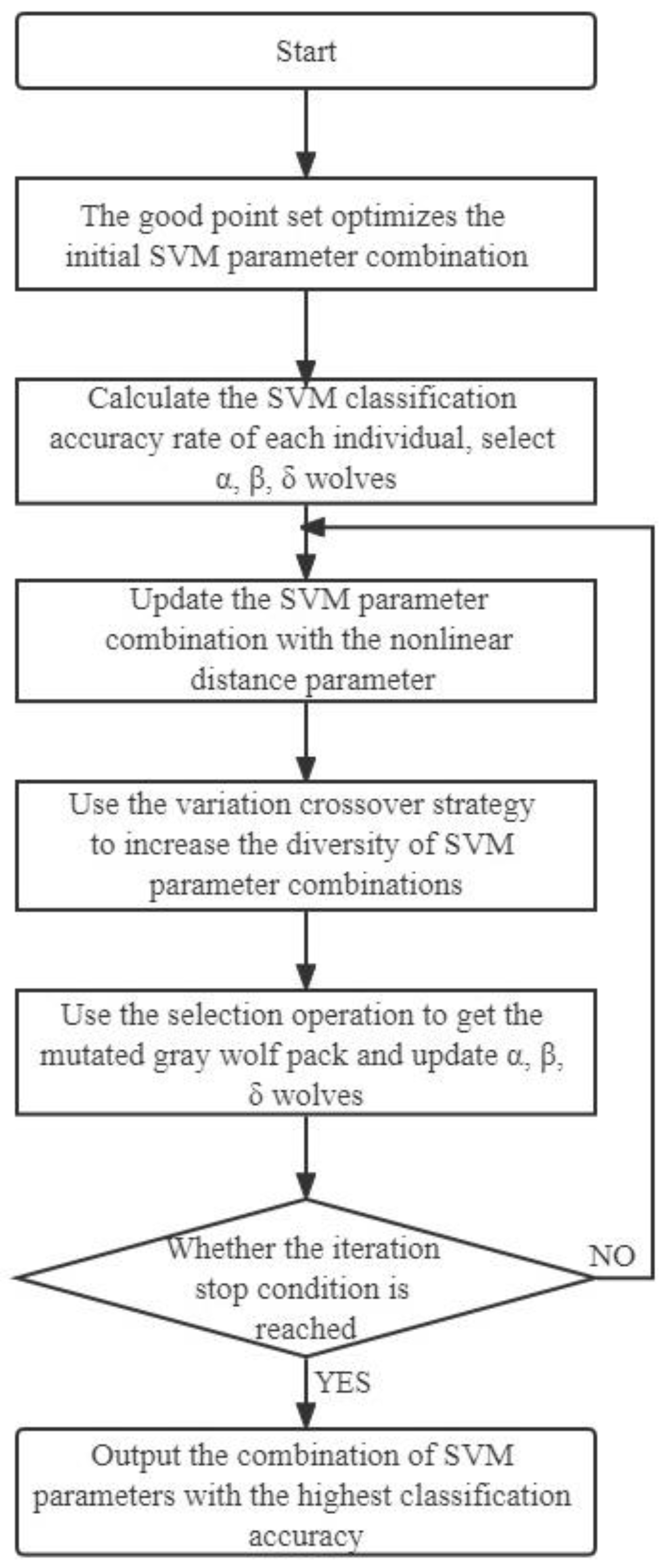
3.3. Improved Gray Wolf Algorithm Optimization Support Vector Machine

Because the penalty factor C and the width g of the radial basis kernel function are difficult to select when the SWM with the radial basis function is used for classification tasks, this paper uses the improved gray wolf optimization algorithm (IGWO) to realize the optimization of SVM parameters based on the radial basis function. The flow of optimizing SVM parameters using the IGWO is shown in Figure 10.

The vibration acceleration data of four modes, including bearing normal, outer ring failure, inner ring failure, and rolling element failure, were selected from Case Western Reserve University under the working conditions of a motor speed of 1750 r/min, a load of 2 HP, and scar depth of 0.1778 mm. A total of 50 sets of data were collected for each working condition, of which, 10 sets of data were used as training groups to train the SVM. The remaining 40 sets of data were used as test groups to test the classification accuracy of the optimized SVM. A total of 40 training groups and 160 test groups were obtained. Aiming at the bearing fault characteristic vector groups obtained by IPSO-VMD combined with sample entropy, the fixed-parameter SVM, GWO-SVM, and IGWO-SVM proposed in this paper were used to classify, respectively.

The fault diagnosis results are shown in

Table 2. Fault diagnosis results with different algorithms.

Method of Fault Feature Extraction	Methods of Fault Diagnosis	Correct Diagnosis of Outer Rings	Correct Diagnosis of Inner Rings	Correct Diagnosis of Rolling Element	Normal State Classification Accuracy Rate	Correct Rate of Overall Diagnosis
IPSO-VMD	SVM	75	100	92.5	100	91.88
	GWO-SVM	85	100	92.5	100	94.38
	IGWO-SVM	92.5	100	100	100	98.13

. In the case of the consistent fault feature extraction method, the fault diagnosis accuracy rate of fixed parameter SVM is the lowest, and the IGWO-SVM greatly improves the accuracy rate of fault diagnosis compared with the GWO-SVM and the SVM with fixed parameters. It is demonstrated that the IGWO-SVM has greater advantages in rolling bearing fault diagnosis.

4. Rolling Bearing Fault Diagnosis Experiment

Under laboratory conditions, the vibration signals of rolling bearings with different fault types were collected based on the test bench, and the acquired data were used to diagnose the fault of rolling bearings by using IPSO-VMD combined with the IGWO-SVM.

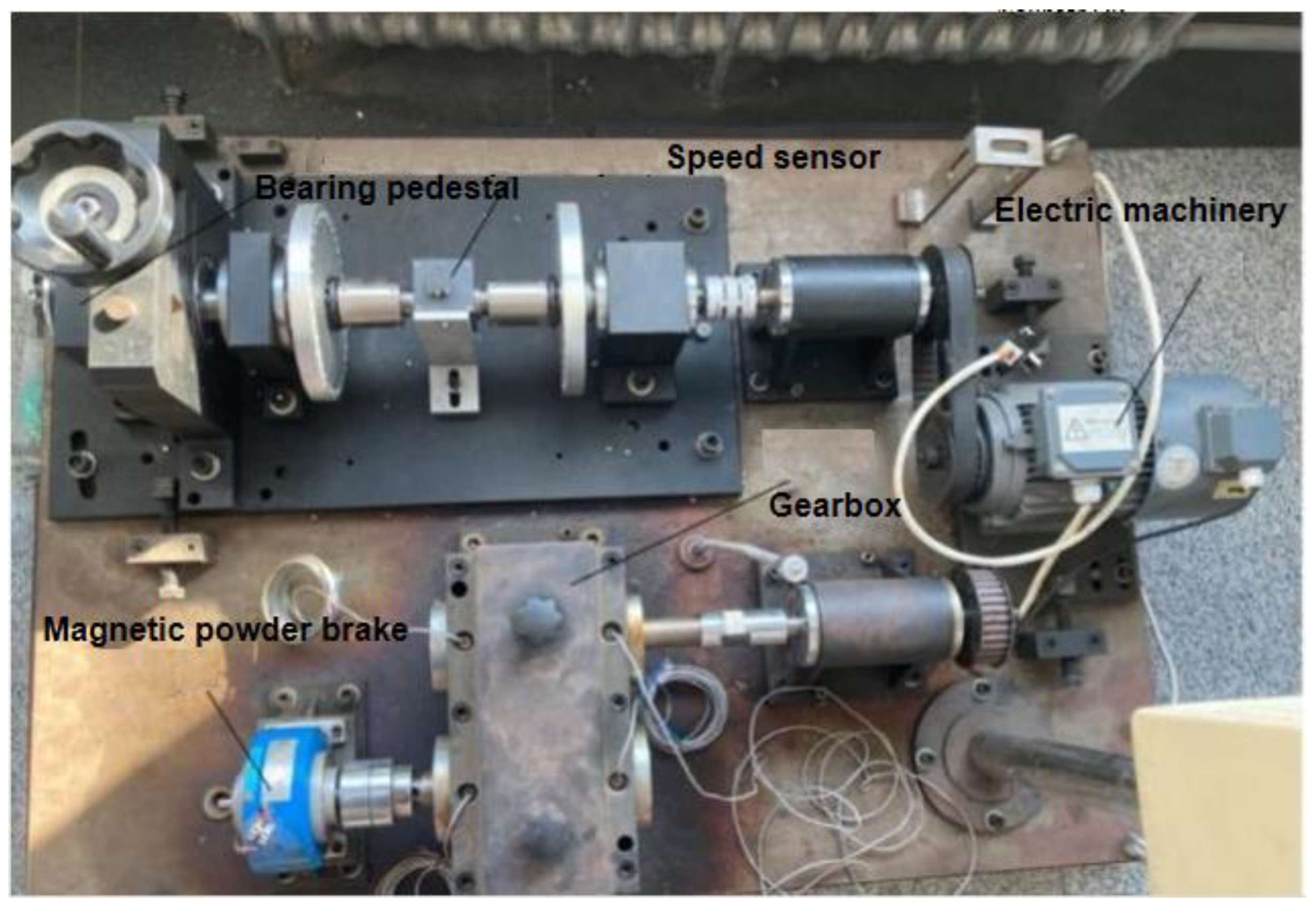
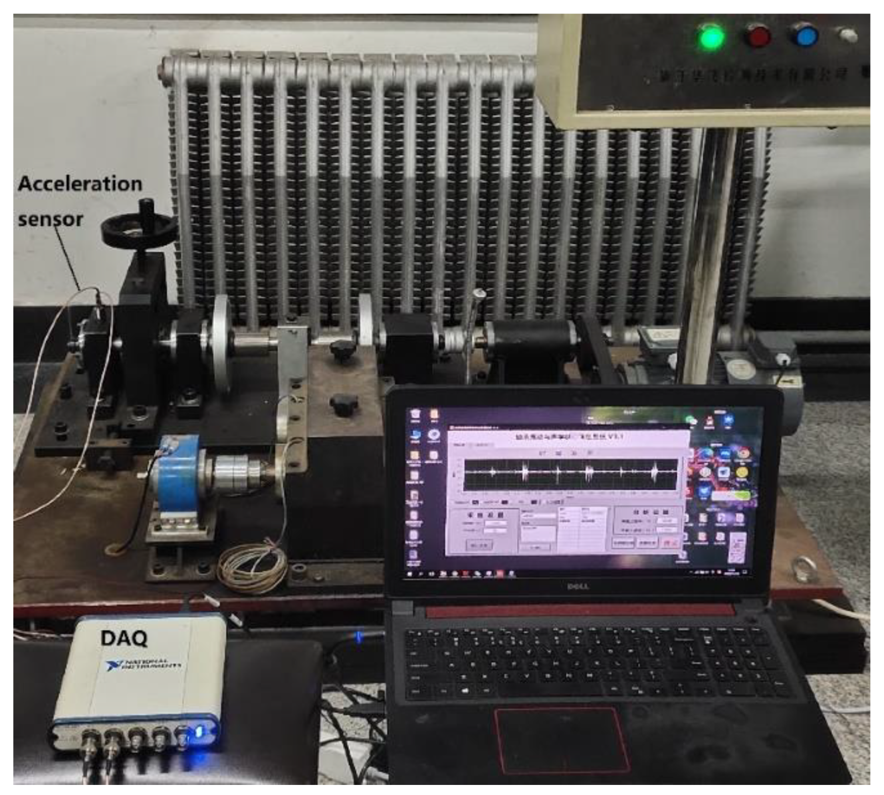
4.1. Experimental Data Collection

The acquisition system was composed of a rolling bearing fault test bench, a vibration acceleration sensor, a rolling bearing with different fault types, and a data acquisition card. The physical diagram of the experimental bench is shown in Figure 11. An AC motor with a rated power of 0.75 kW and a rated voltage of 220 V provided power for the test bench. The maximum speed of the motor was 1450 r/min, and the speed was adjusted by the AC frequency conversion controller. A magnetic powder clutch brake with a maximum torque of 5 N·m was used as the brake of the motor. A JF2100 piezoelectric vibration acceleration sensor with a charge sensitivity of 9.97 mV/ms⁻² was used to measure the acceleration signal.

The rolling bearings used in the experiment were N205 and NJ205, and the bearing specifications are shown in

Table 3. Experimental bearing specifications.

Type	Inner Diameter	Outer Diameter	Rolling Element Diameter	The Number of Rolling Bodies	Contact Angle
N205/NJ205	25 mm	52 mm	8 mm	12	0

below.

In this experiment, the bearing speed was set to 540 r/min. At this speed, the JF2100 sensor was used to measure the vibration acceleration signals. The acceleration signal acquisition system is shown in Figure 12.

The parameter settings of this experiment are shown in

Table 4. Explanation of experimental data.

Bearing Type	Fault Site	Bearing Speed	Each Set of Sample Points	Number of Collected Groups
Cylindrical roller bearings	Raceway surface of the outer ring	540 r/min	4096	50
Cylindrical roller bearings	Raceway surface of the inner ring	540 r/min	4096	50
Cylindrical roller bearings	Rolling element surface	540 r/min	4096	50
Cylindrical roller bearings	No faults	540 r/min	4096	50

.

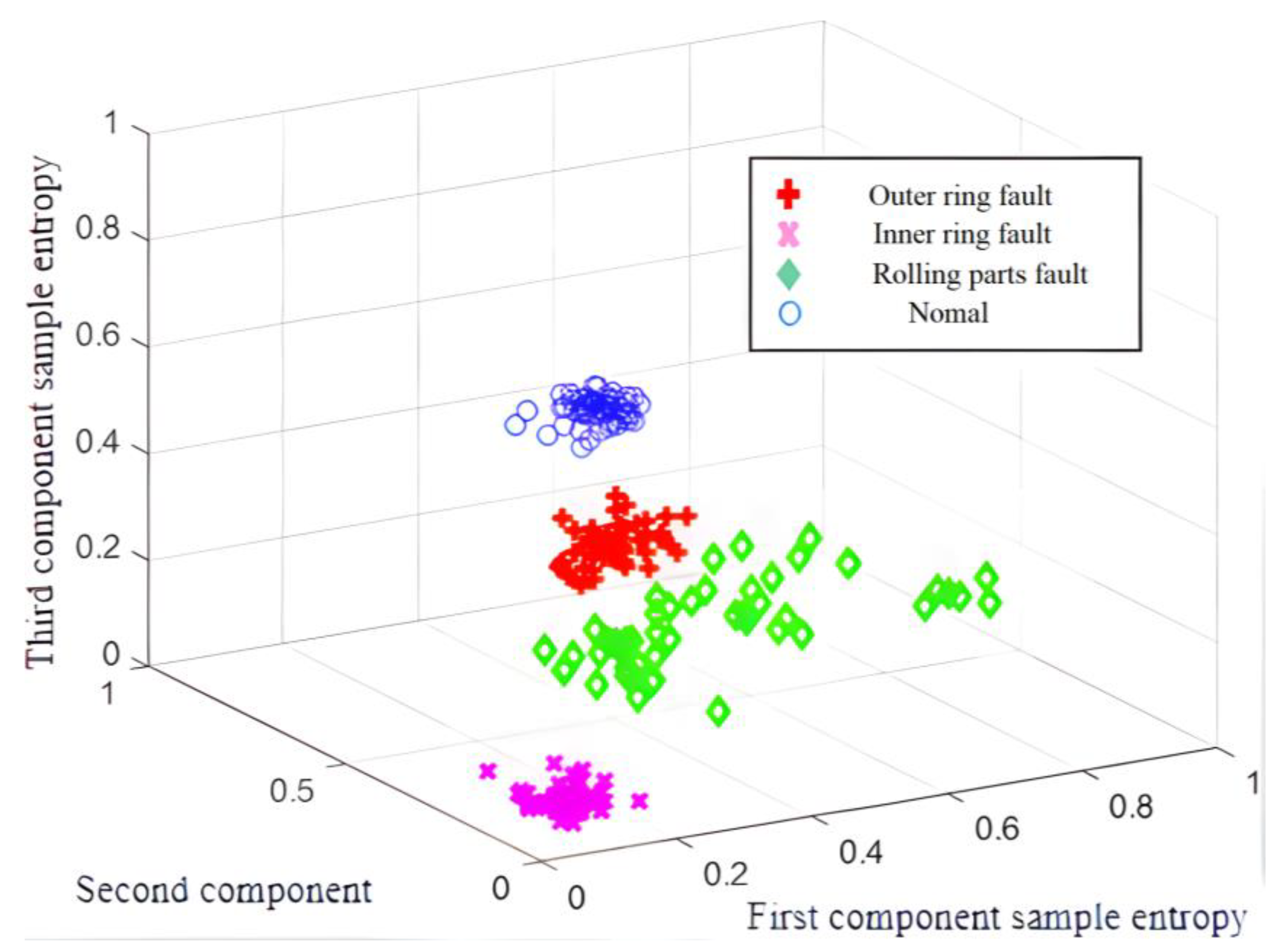
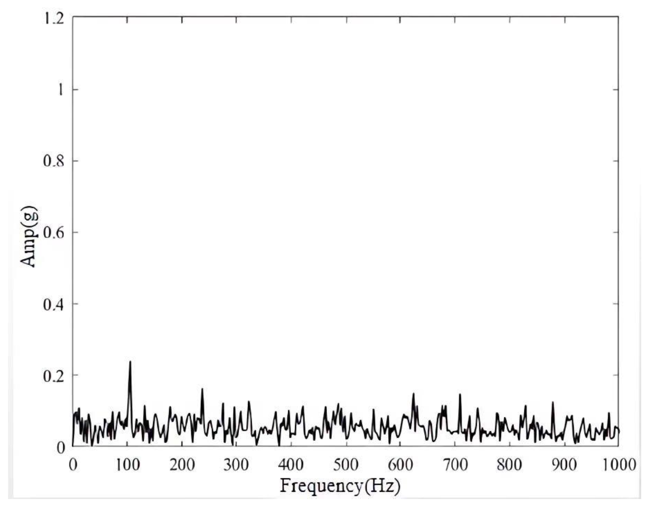
4.2. Fault Feature Extraction of Signals

Using the IPSO-VMD method, 200 sets of data were processed. The VMD parameters of normal bearings, outer ring fault bearings, inner ring fault bearings, and rolling element fault bearings were [8, 466], [10, 9800], [13, 9678], and [5, 466], respectively. The largest three components were selected and processed by the sample entropy algorithm. The embedding dimension m was selected as 2, and the similar tolerance threshold r was selected as 0.2 times the standard deviation, resulting in the bearing fault characteristic vector group of 200 × 3.

Table 5. Rolling Bearing Fault Characteristic Vector Set.

Bearing Type	The First Component Sample Entropy	The Second Component Sample Entropy	The Third Component Sample Entropy	Labels
Outer ring fault bearing	0.2641	0.2844	0.4301	1
	0.2837	0.2919	0.4384	1
	0.2435	0.2613	0.4247	1
Inner ring fault bearing	0.0926	0.0849	0.0798	2
	0.0583	0.2358	0.0699	2
	0.0710	0.0970	0.0629	2
Rolling element fault bearing	0.2259	0.2335	0.3222	3
	0.2532	0.2195	0.2974	3
	0.3060	0.3314	0.3152	3
Normal bearing	0.4643	0.6269	0.5380	4
	0.4174	0.6428	0.5523	4
	0.4015	0.5876	0.4765	4

shows some of the data of the fault feature vector group.

The three-dimensional scatterplot of the fault feature vector is shown in Figure 13. Obviously, the fault characteristics have an excellent accumulation. A rolling element fault bearing has complex components due to the existence of rotation and revolution. However, most of the characteristic points are accumulated in one place, and a small number are scattered. That is to say, it is still significantly different from the fault characteristics of the other three types of bearings. It is proved that the IPSO-VMD algorithm has good fault class discrimination ability.

4.3. Analysis of Fault Diagnosis Results

The IGWO-SVM was used to classify the bearing failure data obtained in the previous section. The first 10 sets of data in each state were treated as training groups to train the SVM, and the remaining 40 sets of data were treated as test groups. In the IGWO, the maximum iterations number was set to 100, the number of populations to 5, the scaling factor range to [0.1, 1.6], the crossing probability to 0.6, the support vector machine’s penalty factor C range to [0.01, 50], and the kernel function’s width g range to [0.01, 50]. The parameters of SVM were optimized by the IGWO. The best penalty factor and kernel function width obtained were 5.2132 and 35.7147, respectively. The SVM was trained with the best parameters obtained by optimization. The trained SVM was used to classify the test set. To fully demonstrate the generality of the experimental results, the IGWO-SVM was used to perform five fault diagnosis experiments on the constructed fault feature vector group.

Table 6. Experiment results of multiple rolling bearing fault diagnosis.

	Accuracy of Outer Rings Diagnosis	Accuracy of Inner Rings Diagnosis	Accuracy of Rolling Element Diagnosis	Accuracy of Rolling Normal State Classification	Accuracy of Rolling Overall Diagnosis
First experiment	97.5	100	100	100	99.375
Second experiment	92.5	100	97.5	100	97.5
Third experiment	97.5	100	100	100	99.375
Forth experiment	100	100	100	100	100
Fifth experiment	97.5	100	95	100	98.125
Average accuracy	97	100	98.5	100	98.875

shows the experimental results. The average accuracy of the five rolling bearing fault diagnosis experiments reached 98.875%, of which, the average fault diagnosis accuracy of the outer ring fault bearing, rolling element fault bearing, inner ring fault bearing, and normal bearing was 97%, 98.5%, 100%, and 100%, respectively. At the same time, the GWO-SVM was used to conduct 5 fault diagnosis experiments on the constructed fault feature vector group, and the average fault diagnosis accuracy for the 5 experiments was 92.375%, which was far inferior to the IGWO-SVM model.

It is shown that the bearing fault characteristics extracted based on IPSO-VMD combined with sample entropy extraction and the bearing fault diagnosis model based on IGWO-SVM can realize the fault diagnosis of the rolling bearing of the bogie of metro trains with stable and high quality.

5. Conclusions

In light of the nonstationary characteristics of the rolling bearings in electric vehicles, the fault signals are complicated and have many interference factors. Taking the rolling bearing of the electric vehicle driving motor as the object, a fault diagnosis method of rolling bearing based on IPSO-VMD and IGWO-SVM is proposed.

In order to determine penalty parameters and the number of decomposition layers, the IPSO-VMD method is proposed by combining IPSO and improved envelope entropy. It optimizes the signal processing effect of VMD. Because the parameters of the SVM have a large influence on the classification effect and are difficult to select, a rolling bearing fault diagnosis model with optimization of SVM parameters by the IGWO based on multiple strategies (IGWO-SVM) is proposed. The algorithm has been compared and verified with public data sets and actual collected data. With the data of Case Western Reserve University with strong noise, the model achieves a diagnostic accuracy of 98.13% compared with the diagnosis accuracy of 94.38% of the GWO-SVM and 91.88% of the fixed parameter SVM. With the actual collected data, the average fault diagnosis accuracy of multiple experiments reached 98.875%. The results show that the IPSO-VMD and IGWO-SVM algorithms have a good effect on the fault diagnosis of rolling bearings with small samples.

References

1. Chen, Q.; Dai, S.; Bi, X. Fault Diagnosis of Rolling Bearings based on EEMD. Comput. Simul. 2021, 38, 361–364, 369. [Google Scholar]
2. Wu, F.; Ding, J.; Liu, S.; Lu, X. Fault Diagnosis of Transmission Shaft System of Automobile based on VMD and PSO-SVM. Mech. Transm. 2019, 43, 120–124, 149. [Google Scholar]
3. Wu, Z.; Huang, N.E. Ensemble Empirical Mode Decomposition: A Noise-assisted Data Analysis Method. Adv. Adapt. Data Anal. 2005, 8, 12–22. [Google Scholar] [CrossRef]
4. Xu, G.; Dai, H. Suspension Fault Diagnosis of Metro Series with EEHD Decomposition and Multi-feature Combination. Mach. Manuf. Autom. 2021, 50, 191–195. [Google Scholar]
5. Konstantin, D.; Dominique, Z. Variational Mode Decomposition. IEEE Trans. Signal Process. 2014, 62, 531–544. [Google Scholar]
6. Liu, C.; Wu, Y.; Zhen, C. Rolling Bearings Fault Diagnosis based on Variational Mode Decomposition and Fuzzy C Means Clustering. Proc. CSEE 2015, 35, 3358–3365. [Google Scholar]
7. Wang, F.; Liu, C.; Zhang, T.; Guo, B.; Han, Q.; Li, H. Fault Diagnosis Method of Rolling Bearing based on k-value Optimization VMD. J. Vib. Test. Diagn. 2018, 38, 540–547. [Google Scholar]
8. Li, H.; Wu, X.; Liu, T. Fault Feature Extraction of Rolling Bearing based on Information Entropy Optimization Variational Mode Decomposition. J. Vib. Shock. 2018, 37, 219–225. [Google Scholar]
9. Zhang, J.; Ji, J.; Xu, T. A Bearing Fault Diagnosis Method based on Variational Mode Decomposition Parameter Optimization. Sci. Technol. Eng. 2021, 21, 3601–3605. [Google Scholar]
10. Chang, Y.; Bao, G.; Cheng, S.; He, T.; Yang, Q. Improved VMD-KFCM Algorithm for the Fault Diagnosis of Rolling Bearing Vibration Signals. IET Signal Process. 2021, 15, 238–250. [Google Scholar] [CrossRef]
11. Zhu, S.; Xia, H.; Peng, B.; Zio, E.; Wang, Z.; Jiang, Y. Feature Extraction for Early Fault Detection in Rotating Machinery of Nuclear Power Plants based on Adaptive VMD and Teager Energy Operator. Ann. Nucl. Energy 2021, 160, 1083–1092. [Google Scholar] [CrossRef]
12. Zhang, Q.; Chen, S.; Fan, Z.P. Bearing Fault Diagnosis based on Improved Particle Swarm Optimized VMD and SVM models. Adv. Mech. Eng. 2021, 13, 1–12. [Google Scholar] [CrossRef]
13. Hao, Y.; Liu, S.; Wu, W. Research on Bearing Vibration Signal Analysis Method Combined with CNN. Mech. Sci. Technol. 2022, 41, 1943–1949. [Google Scholar] [CrossRef]
14. Deng, H.; Zhang, W.X.; Liang, Z.F. Application of BP Neural Network and Convolutional Neural Network (CNN) in Bearing Fault Diagnosis. Mater. Sci. Eng. 2021, 1043, 42–46. [Google Scholar] [CrossRef]
15. Chen, J.; Jiang, J.; Guo, X.; Tan, L. A self-Adaptive CNN with PSO for Bearing Fault Diagnosis. Syst. Sci. Control. Eng. 2020, 9, 11–22. [Google Scholar] [CrossRef]
16. Pinedo-Sanchez, L.A.; Mercado-Ravell, D.A.; Carballo-Monsivais, C.A. Vibration Analysis in Bearings for Failure Prevention using CNN. J. Braz. Soc. Mech. Sci. Eng. 2020, 42, 628–644. [Google Scholar] [CrossRef]
17. Song, L.; Sun, L. Study on Fault Diagnosis Method of EEMD-GSSA-SVM Rolling Bearing. Transducer Microsyst. 2022, 41, 56–59. [Google Scholar]
18. Meng, F.; Du, W.; Gong, X.Y. Fault Identification of Rolling Bearings based on Particle Swarm Optimization Least Squares Support Vector Machine. Bearings 2020, 12, 43–50. [Google Scholar]
19. Chen, Q.; Chen, Z.Y.; Fu, Y. Bearing Fault Diagnosis of Chaotic Bat Algorithm Optimization Correlation Vector Machine. Sens. Microsyst. 2021, 40, 142–145. [Google Scholar]
20. Ma, C.P.; Li, M.H.; Gong, Q.L. Fault Diagnosis of Rolling Bearings of Optimized Support Vector Machine based on Sparrow Search Algorithm. Sci. Technol. Eng. 2021, 21, 4025–4029. [Google Scholar]
21. Zhou, J.; Huang, S.; Wang, M.; Qiu, Y. Performance Evaluation of Hybrid GA–SVM and GWO–SVM Models to Predict Earthquake-Induced Liquefaction Potential of Oil: A Mul-dataset Investigation. Eng. Comput. 2022, 38, 4197–4215. [Google Scholar] [CrossRef]
22. Cui, J.; Zhang, N.; Cui, X. Fault Diagnosis Method of Aircraft Anti-skid Brake System Base on GWO-PNN. In Proceedings of the 2021 33rd Chinese Control and Decision Conference, Kunming, China, 22–24 May 2021; pp. 5402–5406. [Google Scholar]
23. Sharma, S.; Kapoor, A. An Efficient Routing Algorithm for IoT Using GWO Approach. Int. J. Appl. Metaheuristic Comput. 2021, 12, 67–84. [Google Scholar] [CrossRef]
24. Gul, F.; Rahiman, W.; Alhady, S.S.N.; Ali, A.; Mir, I.; Jalil, A. Meta-Heuristic Approach for Solving Multi-Objective Path Planning for Autonomous Guided Robot using PSO–GWO Optimization Algorithm with Evolutionary Programming. J. Ambient. Intell. Humaniz. Comput. 2020, 12, 7873–7890. [Google Scholar] [CrossRef]
25. Ma, R.; Karimzadeh, M.; Ghabussi, A.; Zandi, Y.; Baharom, S.; Selmi, A.; Maureira-Carsalade, N. Assessment of Composite Beam Performance using GWO–ELM Metaheuristic Algorithm. Eng. Comput. 2022, 38, 2083–2099. [Google Scholar] [CrossRef]
26. Hua, Y.; Wang, S.Y.; Bai, G.Z. Improved Particle Swarm Optimization based on Nonlinear Decreasing Inertial Weights. J. Chongqing Technol. Bus. Univ. (Nat. Sci. Ed.) 2021, 38, 1–9. [Google Scholar]
27. Yang, B.; Qian, W. Review of Inertia Weight Improvement Strategies in Particle Swarm Optimization Algorithm. J. Bohai Univ. (Nat. Sci. Ed.) 2019, 40, 274–288. [Google Scholar]
28. Li, L. Application of CEEMDAN method in fault feature extraction and pattern recognition of rolling bearing. J. Lanzhou Jiaotong Univ. 2021, 1, 36–40. [Google Scholar]
29. Li, H.R.; Peng, J. Particle Swarm Optimization Algorithm with Nonlinear Inertial Weights and Cauchy Variation. Comput. Digit. Eng. 2021, 49, 1325–1329, 1362. [Google Scholar]
30. Huang, J.; Guan, Y.N. SVM Parameter Optimization Method based on Good Point Set Particle Swarm Algorithm. J. Packag. 2019, 11, 74–80. [Google Scholar]
Figure 1. The Fault Feature Extraction Algorithm Flow Chart based on IPSO-VMD.
Electronics 12 01290 g001
Figure 2. Time Domain Diagram of Outer Ring Fault Signal.
Electronics 12 01290 g002
Figure 3. Time Domain Diagram of Outer Ring Fault Signal with Strong Noise.
Electronics 12 01290 g003
Figure 4. Outer ring fault signal envelope with strong noise added.
Electronics 12 01290 g004
Figure 5. IPSO-VMD fitness iteration graph.
Electronics 12 01290 g005
Figure 6. IPSO-VMD Optimum Component Envelope Spectrum.
Electronics 12 01290 g006
Figure 7. Fixed parameter VMD optimal component envelope spectrum.
Electronics 12 01290 g007
Figure 8. Optimal component envelope diagram of EMD.
Electronics 12 01290 g008
Figure 9. Nonlinear distance parameters and linear distance parameters comparative analysis.
Electronics 12 01290 g009
Figure 10. Improved Grey Wolf Algorithm to Optimize SVM Parameter Combination Process.
Electronics 12 01290 g010
Figure 11. Test bench for rolling bearing fault diagnosis.
Electronics 12 01290 g011
Figure 12. Acceleration signal acquisition system.
Electronics 12 01290 g012
Figure 13. IPSO-VMD component sample entropy map of different state signals.
Electronics 12 01290 g013