Research on Railway Obstacle Detection Method Based on Developed Euclidean Clustering

Abstract

To prevent the problem of safety accidents caused by the intrusion of obstacles into railway clearance, this paper proposes an obstacle detection method based on Light Detection and Ranging (LiDAR) to obtain and process rich three-dimensional (3D) information and depth information of the railway scene. The method first preprocesses the point cloud of the railway scenario collected by LiDAR to divide a basic area containing the rails. Then, the method divides the roadbed plane and fits the rails with the random sample consensus (RANSAC) algorithm, dividing the detection area according to the position of the rails. To address the issue of over or under-segmentation in the traditional Euclidean clustering method, which is due to sparser point clouds the farther the object is from the LiDAR, this paper improves the conventional Euclidean clustering. It introduces an adaptive distance threshold to categorize obstacles. Finally, compared with traditional Euclidean clustering, K-means clustering, and density-based spatial clustering of applications with noise (DBSCAN) clustering, the improved Euclidean cluster has achieved better results in terms of computing time and segmentation accuracy. Experimental results show the ability of the method to detect railway obstacles successfully.

1. Introduction

Railway transport safety is essential to many rail transport systems, as trains constantly increase in quantity, volume, and speed [1]. Railway accidents damage people’s lives, reduce driving efficiency, and waste many resources. With random, sudden, and unpredictable characteristics in railway foreign object invasion, railway safety accidents easily occur because it is difficult for drivers or workers to find obstacles in time. There needs to be active and effective supervision of the railway locations prone to foreign item incursion. Consequently, railway accidents caused by obstacles are one of the most critical issues that should be solved. How to detect foreign objects in the railway in real-time, efficiently, and accurately has become a research question.

Aiming to achieve a pleasing effect of railway obstacle detection, many researchers propose solutions. A frequently used solution is to obtain foreign object information through direct or indirect contact between sensing elements and foreign objects. Such an approach detects obstacles using a leaking coaxial cable or grating sensor. The method based on leaky coaxial cables performs well in actual applications [2], and the grating sensor detection method is an effective instrument for detecting intruders [3]. Unfortunately, such a contact detection approach takes up a lot of space and has a limited detecting range. Hence, in many scenarios, non-contact detection is desirable. Specifically, ultrasound creates a detection system based on complementary sequences for signal processing and coding [4]. This method resists transmission signals and random fluctuations when detecting objects falling on the railway, but the detection range is limited. Recently, the most popular algorithm has been the pattern recognition detection algorithm that utilizes sensors such as cameras. The Fast Region-Convolutional Neural Network (R-CNN) network model is used to solve the problem of front vehicle detection in traffic situations [5]. The successful implementation of this technique partially overcomes the problem of foreign object occlusion, and the algorithm successfully reduces the false detection rate while increasing detection accuracy. The detection accuracy is higher than directly using the Convolutional Neural Network (CNN). Someone else presented an enhanced Cascade Mask R-CNN (CMR) model, which improves small target detection accuracy [6]. Although the video detection algorithm has been dramatically developed and achieved good results, in practice, haze can reduce the camera’s detection performance. In contrast, LiDAR can reflect the 3D information of objects and can work all day. Our design avoids the influence of point cloud sparsity and reduces workload.

There are three frequently used clustering methods of point cloud segmentation. First, researchers can segment the point cloud by density, such as the DBSCAN clustering algorithm [7,8]. Many application scenarios have achieved good results but are challenging when dealing with large amounts of data. Second, there is an iterative algorithm for randomly choosing cluster centers [9,10]. When such a clustering algorithm is applied to the field environment, the method’s K (the number of clusters) value may not correspond to the number of obstacles—the obstacle detection system would be required to set the K value manually. Third, traditional Euclidean clustering is straightforward and efficient [11], but the fixed distance threshold causes under-segmentation or over-segmentation in point cloud data with uneven density. Various surveys explored aspects of the problem, including dividing different regions according to distance and setting the clustering distance threshold according to the experimental results [12]. Algorithms that use point cloud depth information to segment regions must traverse each point and determine the threshold setting through several trials. Setting the adaptive threshold directly based on the trial outcomes takes a lot of effort.

The proposed railway obstacle detection system combines the advantages and disadvantages of the above methods: it provides an improved Euclidean clustering with a distanced threshold determined by the LiDAR’s parameters to eliminate the problem of over-segmentation and under-segmentation. However, it requires well-divided regions of interest (ROI) before clustering. We achieved good detection results by fitting the rails to divide the ROI using the RANSAC algorithm.

The contribution of this study is to design a railroad obstacle detection system that analyzes the unique characteristics of railroad point cloud data. By mounting the LiDAR at the trackside platform, such as a signal pole, the LiDAR transforms the scene around that platform into 3D point cloud data, and we use the data to detect obstacles. RANSAC is used to divide the ROI for better results. Another contribution is to propose and compare the improved Euclidean clustering method with other methods to prove its effectiveness in obstacle segmentation.

2. Related Work

Our work involves the application of LiDAR obstacle detection technology in railway sites. Therefore, the related work is divided into two parts. The first part discusses the research on orbital obstacle detection, and the second part includes related algorithms for LiDAR detection of obstacles.

2.1. Railway Obstacle Detection

Railway traffic safety has been a large concerned since the railway was built, among which obstacle detection is a challenge in the safe operation of the railway, and there are many important kinds of research. Early railway obstacle detection is to obtain obstacle information through direct or indirect contact between the power grid or grating and foreign objects. The data processing of this kind of method is relatively simple, and the technology is relatively mature. Although this method can determine the obstacle intrusion event to a certain extent, the equipment installation is complicated, the investment is huge, the detection range is limited, and we cannot determine the type of obstacle intrusion.

Because of the disadvantages of contact detection methods, non-contact detection methods have emerged. This method uses the transmission characteristics of electromagnetic waves and sound waves to obtain information about obstacles without touching the measured object’s surface. The obtained data contains a lot of information, and data processing is relatively complex. Some researchers have adopted thermal imagers to detect objects near railway tracks [13,14]. Such methods have achieved good results in low-light environments and in detecting biological obstacles. However, they cannot detect obstacles at the same temperature as the environment or provide any depth information.

Many vision-based object or foreign object detection methods have been developed in the railway field [15,16,17,18,19,20,21]. These methods usually use artificial intelligence and computer vision methods for obstacle detection. Among these methods, the camera-based target detection algorithm is one of the most active research fields in computer vision [22,23,24,25,26], and many methods achieved some success. Unlike cameras, LiDAR sensors can provide precise distance information for objects and are already widely used.

Others have developed an advanced sensor setup that combines cameras, thermal imagers, and LiDAR to detect objects in orbit [27,28,29,30]. Many people use the fusion of LiDAR sensors and cameras to obtain depth information on obstacles. The obstacle information obtained by multi-sensor fusion contains more content, which can detect obstacles more accurately and distinguish obstacle categories, but at the same time increases the construction cost of the detection system and the algorithm’s complexity.

In the above method, the data acquired by the LiDAR sensor can not only visualize the shape of the obstacle but can also obtain the object’s depth information and calculate the object’s running speed. It is also applicable in the case of dim light. Therefore, the detection of obstacles by LiDAR algorithmic research is necessary.

2.2. Algorithm of LiDAR

2.2.1. Segment the Ground

Ground points comprise a relatively large portion of the 3D data, but are not points on obstacles. Therefore, ground points must be removed before obstacle detection to obtain more accurate detection results. Many researchers have studied this, and one strategy is the raster map approach. This method usually uses the height value in the grid as the basis for judgment. Some screen out the ground based on the height difference [31], and some extract the ground based on the average height [32]. These methods can effectively eliminate noise points, but they do not use the continuity information of the ground to segment the ground, which is less robust and susceptible to under-segmentation problems caused by environmental influences.

To make full use of the continuity characteristics of the ground, relevant scholars have carried out research on the aspects of line-based fitting and plane-based fitting [33]. Himmelsbach constructed a polar grid map [34]. This method uses the incremental straight-line algorithm to segment the candidate ground points in the grid, which has high efficiency and does not require high precision of the laser radar. However, it cannot detect the sloping plane well.

The ground segmentation algorithm based on plane fitting assumes that the ground is a plane and uses the plane fitting algorithm to segment the ground. The simplest method is the RANSAC algorithm, which uses random sampling to fit the plane to the ground [35]; this has been widely used and has achieved better results when the ground is close to the plane.

2.2.2. Model Fitting

The model fitting method realizes the point cloud segmentation through the model fitting of the point cloud data and the preset value. Among them, the widely used and effective methods mainly include the 3D Hough transform [36], the random sampling consensus algorithm [37], and their extended algorithms.

HOUGH proposed the Hough transform in 1962, a purely mathematical method for transforming parameter spaces [38]. This algorithm maps points from 3D space to parametric space for voting by changing the mathematical representation of the points. It has good detection results for various parametrizable shapes. Researchers have used it to extract the boundary lines of architectural point clouds [39,40] with good experimental results.

The random sampling consensus algorithm selects multiple subsets in the point cloud to fit the model and selects the model with the best fitting effect as the fitting result. The RANSAC algorithm is simple yet powerful and is widely used [41]. In 2007, TARSHA-KURDI et al. [42] of the French National Institute of Applied Sciences compared the 3D Hough transform and the RANSAC algorithm. Experiments proved that the RANSAC algorithm has higher efficiency and accuracy. However, the random sampling consensus algorithm’s time complexity is high and unsuitable for large-scale domains. Therefore, in this paper, we use this algorithm after filtering the original data, effectively reducing the computation time.

2.2.3. Obstacle Detection

The obstacle detection algorithm of the point cloud mainly includes some clustering algorithms. The principle of cluster analysis is to gather samples with large similarities into the same class so that the similarity of samples in the same class is as large as possible and the similarity between different classes is as small as possible to reveal the actual situation of these data distributions.

The DBSCAN algorithm is a density-based clustering algorithm that can quickly cluster point cloud data of any shape [43]. For each object in a certain cluster, the number of data objects must be greater than a given value within the area of a given radius. That is, the neighborhood density must exceed the density threshold. The algorithm finds arbitrary objects from a dataset and finds objects in the dataset that satisfy a given radius and density threshold to form clusters. This method consumes a lot of memory when the number of point clouds is large.

The k-means clustering algorithm can ensure the accuracy and efficiency of clustering results when the number is huge [44]. It requires input sample data and the number of clusters K. Then, select K objects in the sample as the initial cluster, calculate the position of the center point of each cluster, and calculate all points in the sample. Take the distance to each center point and re-divide the minimum distance point; then, recalculate the center point position of each cluster and the distance from all points in the sample to each center point, re-divide the minimum distance point, and repeat the calculation. Repeat these steps using the position of each cluster center point until the cluster no longer changes. This method needs to manually input the number of clusters K, which is not applicable in the obstacle monitoring environment with a complex environment.

The clustering analysis based on the depth image integrates the depth information in the point cloud information for clustering processing. This method is more accurate for positioning the target but requires a lot of data support [45]. If the data is insufficient, achieving the desired effect is not easy.

The Euclidean clustering algorithm is simple and efficient, with powerful point cloud segmentation ability and good real-time performance. It has high reliability in normal scenarios and does not require huge data support [46]. This method performs clustering by computing and comparing the Euclidean distance between each point and its neighbors.

3. System Architecture

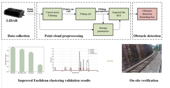
Figure 1 depicts the block diagram of the obstacle detection system. The system consists of three modules: data collecting, segmenting the ROI, and obstacle detection. In the first module, we describe a sensor system consisting of a 3D LiDAR and a device for storing data in three dimensions. A method for segmenting out railway boundaries is proposed in the second module. Here, points on the rail are extracted and utilized to segment track limits. An improved Euclidean clustering algorithm for obstacle segmentation is presented in module three for a clear detection result, including 3D information on objects.

4. Segment the ROI

Thousands of points are required to describe a railway scene using a data set of 3D points. The more points in the data set, the more sophisticated the algorithm, the longer the time required, and the interference of noise points will reduce detection accuracy. As a result, good boundary area division can enhance detection speed and accuracy.

Design of a detection region segmentation scheme using the RANSAC algorithm, as shown in Figure 2. First, use a straight-through filter to extract the area of the rail. Perform one pass on the result to obtain as many points on the rail as possible to obtain a more accurate division effect, then obtain points on the rail by eliminating ground points with the RANSAC algorithm. In the second step, fitting points on rails with the RANSAC algorithm is essential for segmenting the area of interest. Then, position the points on the rail by the rail’s shape. The third type is to segment the ROI with the parameters obtained by fitting.

4.1. Preprocess the Point Cloud

A pass-through filter divides the rails’ position:

$$\left\{\begin{array}{l}\min x\le x\le \max x\\ \min y\le y\le \max y\\ \min z\le z\le \max z\end{array}\right.$$

(1)

In Figure 3, $\min x,\max x,\min y,\max y,\min z,\max z$, and max z refer to the 3D Cartesian coordinate system’s maximum and minimum coordinate values. Figure 3 shows a 3D cuboid with required interior and surface points (green points) and eliminated outer points (red points).

4.2. The RANSAC Algorithm for Subgrade Plane Segmentation

The key to the second module is to determine the position of the rails. Divide the railway boundary region after determining the location of the railway line with two rails. The method in this paper takes advantage of the fact that the surface of the rails is much higher than the base plane to extract the rails points; when we remove the base plane, most of the remaining points are rails points.

After dividing the position range of the rail, use the RANSAC algorithm to remove the subgrade plane. Bolles and Fischler applied RANSAC to solve the real problem [47]. The RANSAC algorithm randomly selects a portion of a given data point sample to calculate model parameters; then, using the consequent model, it calculates the distance from other points to the model. Check whether the distance is inside the specified threshold range; if so, the point is interior, and if it is not satisfied, it is an outlier point. Continue selecting sub-samples randomly and repeating the preceding procedures until it reaches the specified number of iterations; compare and select the model parameters with the most interior points and output.

Calculate the number of iterations theoretically [47],

$$SD\left(k\right)=\frac{\sqrt{1-{\mathsf{\omega }}^n}}{{\mathsf{\omega }}^n}$$

(2)

where $k$ is the number of iterations, and $\mathsf{\omega }$ is the ratio of interior points to the number of points in the data set. Assuming that $n$ points are selected for the estimation model, then ${\mathsf{\omega }}^n$ is the probability that all points are internal points.

To fit a plane using the random consensus algorithm, the algorithm selects three points, $p_1$, $p_2$, and $p_3$, in the point cloud dataset, and their coordinates are $(x_1,y_1,z_1)$, $(x_2,y_2,z_2)$, and $(x_3,y_3,z_3)$. Three points form a plane:

$$Ax+By+Cz+D=0$$

(3)

$$\left\{\begin{array}{l}A=\left(y_2-y_1\right)\left(z_3-z_1\right)-\left(y_3-y_1\right)\left(z_2-z_1\right)\\ B=\left(x_3-x_1\right)\left(z_2-z_1\right)-\left(x_2-x_1\right)\left(z_3-z_1\right)\\ C=\left(x_2-x_1\right)\left(y_3-y_1\right)-\left(x_3-x_1\right)\left(y_2-y_1\right)\\ D=-\left(A{x}_1+B{y}_1+C{z}_1\right)\end{array}\right.$$

(4)

The distance from another point $p_4(x_4,y_4,z_4)$ in space to this plane is:

$$s=\frac{\left|A{x}_4+B{y}_4+C{z}_4+D\right|}{\sqrt{A^2+B^2+C^2}}$$

(5)

Repeat the above steps to select the best plane fitting result, the parameters with the most points in the plane. When $s$ is less than the specified distance threshold, $p_4$ is an inner point. Otherwise, it is an outlier point.

4.3. The RANSAC Algorithm for Fitting Points on the Rails

Because there are still numerous noise points on the rail after eliminating the subgrade plane, the RANSAC method is used to fit the noise points. This noise point ignoring algorithm prevents us from being confused by other points before getting the ROI [47]. It allows us to remove noisy points while leaving points on the rails. Moreover, we can fit straight rail lines or curves depending on the rail shape. Then, segment the ROI according to the parameters obtained by fitting. Figure 4 presents a data set of rail points projected on the ground. Because we intend to fit one of the lines, points on the other rail and others are considered noise points. Figure 4 is a practical example where the impact of noise points on linear regression is far higher than that of the RANSAC algorithms.

Fitting the rails also uses a random sampling consensus algorithm. The algorithm steps are the same as the ground plane fitting. The difference is that the algorithm needs to randomly select two points to fit a straight line and select three points to fit an arc. Thus, for a straight line, Equation (6) appears, and for a circle, Equation (7) appears.

$$\frac{x-x_5}{m}=\frac{y-y_5}{n}=\frac{z-z_5}{p}$$

(6)

$$\left\{\begin{array}{l}{\left(x-x_6\right)}^2+{\left(y-y_6\right)}^2+{\left(z-z_6\right)}^2=r^2\\ a\left(x-x_6\right)+b\left(y-y_6\right)+c\left(z-z_6\right)=0\end{array}\right.$$

(7)

where $(x_5,y_5,z_5)$ is the coordinates of a point on the line, $(x_6,y_6,z_6)$ is the coordinates of a point on the circle, $(m,n,p)$ is the direction vector of the line, $(a,b,c)$ is the normal vector of the plane on which the circle lies, and r is the radius of the circle.

4.4. Segment the ROI

Figure 5 shows the basis for dividing the ROI area. First, this method projects all points to the rail plane (fixed LiDAR installation location, which is the ground plane) and projects the linear and circular arc equations to this plane. Then, find another rail’s approximate location using the two rails’ approximate parallel characteristics. Finally, divide the detection area according to the specified range (red area in Figure 5).

5. Improved European Clustering

5.1. Algorithm Principle

5.1.1. Building a Kd-Tree

The point cloud data are often uneven, noisy, and large. The clustering algorithm requires determining the search relationship between discrete points. Hence, it is necessary to establish a point search relationship, such as kd-trees.

Kd-trees extend binary search trees to the multi-dimensional data structure, which realizes the organization and storage of primarily spatial data [48,49]. Therefore, the kd-trees are essentially a binary search tree, which satisfies the properties of a binary search tree. Kd-trees exhibit the following prominent properties:

• If a node’s left or right subtree is not empty, then all node values on the left subtree are smaller than this node, and all points on the right subtree are bigger than this node value.
• The subtree of any node is also a binary tree.
• It can efficiently deal with unevenly distributed data.
• Since the point cloud data are 3D, the established kd-tree extends the binary tree to 3D space. Each tree point divides the 3D space into two parts, and this approach finds the discrete points near a point quickly by comparing the three dimensions separately. At the same stage in the 3D KD tree, only compare the value of the root node and the child node of one dimension. Figure 6 shows an example of the search process. The data in each box of the graph represent the 3D coordinates of a point, and each layer represents one dimension.

5.1.2. Euclidean Clustering with Adaptive Distance Threshold

The structure of the traditional Euclidean algorithm is simple and efficient. First, select a central point named $q_{11}$ from a point cloud data, then look for $n$ points near the center point. If the Euclidean distance between two points satisfies the threshold $\delta$, put it in the cluster $E$ and mark it, such as $q_{12}$, $q_{13}$, and $q_{14}$. Second, find a point $p_{12}$ in $E(q_{11})$, repeatedly find the nearest $n$ points that meet the distance threshold, add them to $E(q_{11},q_{12})$, and repeatedly find the points that meet the distance threshold and put them into class $E$. The algorithm’s search is complete when there are no new points to add to $E$.

We note that a fixed distance value of $\delta$ must be set for the traditional process. The farther away from the LiDAR, the smaller the density of the point. Therefore, a fixed distance cannot satisfy all location clustering, resulting in over-segmentation and under-segmentation. The key idea is to set the adaptive distance threshold to achieve good segmentation.

The Euclidean distance of two points in 3D space is:

$$\mathsf{\rho }=\sqrt{{\left(x_2-x_1\right)}^2+{\left(y_2-y_1\right)}^2+{\left(z_2-z_1\right)}^2}$$

(8)

where a and b are the coordinates of two points.

The following equation calculates a variable distance constraint $d_t$ for the improved Euclidean clustering:

$$\left\{\begin{array}{l}{d}_t=a\sqrt{h_0{}^2+v_0{}^2}+t_0\\ h_0=2d_0\tan \left(\alpha /2\right)\\ v_0=2d_0\tan \left(\beta /2\right)\end{array}\right.$$

(9)

where $a$ is a tuning parameter and $t_0$ is an adjustment function. $\alpha$ is the horizontal resolution, and $\beta$ is the vertical resolution. This LiDAR’s horizontal and vertical resolution values are 0.18° and 0.24°. As illustrated in Figure 7, we map the threshold setting problem into a geometric analytical figure. Considering $V$ as a location of the LiDAR and $s_1$, $s_2$, and $s_3$ as the rays emitted by the LiDAR. $F$ is a face of an obstacle facing the LiDAR, is $d$ meters away from the LiDAR, blocks three rays, and generates points $q_1$, $q_2$, and $q_3$. $B$ and $C$ are the midpoints of the line connecting the two points. Therefore, $h_0$ is the horizontal length of the rectangle when the distance from the LiDAR is $d_0$; $v_0$ is the vertical length of the rectangle in the figure when the distance from the LiDAR is $d_0$, where $d_0$ is equal to $d$, which is the distance between the index core point and the LiDAR.

5.2. Algorithm

Let $P$ denote the data set input to the algorithm and $C$ to the matrix output by the algorithm representing the clustering result.

• Create a kd-tree index for $P$ and initialize a cluster $C$.
• Define a seed queue $Q$, add the $i$th point $p_i$ in the point set $P$ to the queue, search for the point adjacent to $p_i$ and calculate the Euclidean distance $d_e$ between the two points. If the distance satisfies $d_e\le d_t$, add the adjacent point to the queue; Select the neighbors of all points in the queue to join the queue until there are no more points to join.
• After step 2, group the points in queue $Q$ into a category. If the number $n$ of points in $Q$ satisfies the condition of $N_{\min }\le n\le N_{\max }$, put $Q$ into the cluster $C$; otherwise, it will not be stored.
• Clear $Q$ to zero, continue to index other points that have not been processed, and repeat steps 2 and 3 until all points have been processed.

5.3. Bounding Box

According to the clustering results, we added an axis-aligned bounding box (AABB) to each obstacle to clearly describe the 3D information of the object. The specific implementation process traverses each cluster’s points, comparing the cluster midpoints’ 3D extreme values, and making a hexahedral bounding box with the finally obtained values.

6. Experiments and Results

6.1. Experimental Data Preparation

6.1.1. Euclidean Clustering with Adaptive Distance Threshold

To verify the effectiveness of the method proposed in this paper, we arranged obstacles such as cardboard boxes, backpacks, and pedestrians in the actual railway scene to collect experimental data. A LiDAR named Falcon Kinetic from Innovusion is a tool that collects point cloud data, and we mounted it on a stand at a trackside height of approximately 2.5 m. The experimental platform was Ubuntu 18.04. The programming language was Python 3.9.

6.1.2. Data Preprocessing

This experiment contains two data sets, dataset 1 and dataset 2.

Dataset 1 is the result of preprocessing 100 frames of original point cloud data. We use it to verify the improved Euclidean clustering. In Figure 8, there is the process of data preprocessing. There are many noise points in the railway data set (e.g., Figure 8a). This problem causes difficulties in detection. To solve this problem, we extracted the points on a rail (e.g., Figure 8b) and used these points to segment the ROI (e.g., Figure 8c). Therefore, to prepare data for experiments, we considered the points after going to the ground as obstacles (e.g., Figure 8c) and stored them in dataset 1.

For the experiment (to test the performance of our proposed scheme in actual application scenarios), we used dataset 2 of 6395 frames point cloud, collected from railway scene data. There were 2930 frames of data without obstacles and 3465 frames containing obstacles, and the obstacles were all within 100 m of the LiDAR. There were 1995 frames of carton data, 1830 frames of pedestrian data, and 175 frames of train data.

6.2. Cluster Segmentation Experiment

This section shows and discusses the comparison results of K-means, DBSCAN, Euclidean, and improved Euclidean. The input to the experiment is dataset 1 of obstacles containing point clouds on obstacles. The results after clustering and segmentation could be more precise and add bounding boxes, as shown in Figure 9. The bounding box helps us observe the point cloud segmentation and obstacles’ size and position information. We set the fixed distance threshold to 0.2 for the other three algorithms in our experiments.

6.2.1. Segmentation Accuracy

A comparison of four methods, K-means clustering, DBSCAN clustering, Euclidean clustering, improved Euclidean clustering, and actual load, is shown in Figure 10. Figure 11 shows the correct rate of every method, that is, 0.24, 0.89, 0.71, and 0.82. Since the K-means algorithm needs to specify the number of clusters K, but the actual number of obstacles is not fixed, K is specified as the average value of obstacles in the experiment.

6.2.2. Algorithm Time-Consuming Analysis

Figure 12 and Figure 13 depict the time-consuming result of the above clustering algorithms. Figure 12 shows the overall time consumption of each algorithm. The places where the data changes significantly in the figure are the train data. Due to the large size of the train, the number of points on the train is large, which leads to a longer calculation time for the clustering algorithm. As the amount of data increases over time, the DBSCAN algorithm takes the longest, and K-means clustering takes the shortest. Euclidean clustering and improved Euclidean clustering are in the middle. Figure 13 shows the average time-consumption of the four algorithms. Both Euclidean clustering and improved Euclidean clustering have obtained good verification results.

6.2.3. Overall Performance Analysis

The comparison results exhibit the following:

• K-means clustering algorithm operation time is short. However, in practical applications, it is only sometimes applicable to input the units of the clustering results.
• Although the DBSCAN clustering algorithm has the highest accuracy, the running time of this algorithm calls for more studies and improvements. This does not meet real-time requirements.
• Compared with the traditional Euclidean clustering, the operation time of the improved Euclidean clustering is similar, and 11 percentage points increase in the segmentation accuracy.

6.3. Field Experiment Verification

Table 1. Test result.

Distance Between Obstacles and LiDAR (m)	Carton Detection Rate (50 × 50 cm) (%)	Pedestrian Detection Rate (Height 175 cm) (%)	Train Detection Rate (%)
$d<50$	84.33	98.04	100
$50\le d<80$	61.25	86.42	100

shows that the farther away the obstacle is from the LiDAR, the smaller the area and the lower the obstacle detection accuracy rate is. We found three main reasons for this detection problem. One of the reasons is the size of the obstacles. As the area of the object decreases, the points on the obstacle become less and less, affecting the detection effect. Another effect happens due to the distance between the LiDAR and obstacles. The farther the distance, the sparser the points. In addition, the problem with low obstacle height is that it can cause points on obstacles with an enormous specific gravity to segmented when segmenting the ground.

7. Conclusions

Safety is essential in railroad operation, and obstacle intrusion seriously affects traffic safety. To improve the accuracy and efficiency of railway obstacle detection, we propose an efficient railway obstacle detection method in this paper. This method uses the RANSAC algorithm to segment the ROI and the improved Euclidean clustering to solve the problems of over-segmentation and under-segmentation. Experimental results show that this algorithm can segment ROI accurately and has better detection results.

The method uses the RANSAC algorithm to determine the rail position after dividing the roadbed plane and then dividing the ROI according to the rail position. Figure 8 shows the specific experimental procedure and that the segmentation works well.

We propose an improved Euclidean clustering algorithm for segmenting obstacles. This algorithm differs from other clustering algorithms because the distance threshold is variable, so that it can segment inhomogeneous point cloud data. We tested the segmentation effect of the improved Euclidean clustering and the other three algorithms (DBSCAN algorithm, Euclidean clustering algorithm, and K-means algorithm) with 100 frames of data containing obstacles. The experimental results showed that the K-means algorithm is not applicable in practical applications because the number of obstacles cannot be determined. The DBSCAN algorithm rapidly increases the operation time when data increases. The improved Euclidean clustering has a longer operation time than the traditional one, but the correct segmentation rate increases by 11 percentage points. Considering the operation time and correct rate together, the improved Euclidean clustering algorithm is better. The detection results of testing the whole system with raw point cloud data show that the closer the obstacle is to the LiDAR, the larger the area, and the higher the height, the better the detection results. In addition, it shows that actual railroad scenes can achieve good results with this algorithm for obstacle detection.

We plan to continue the development of this research, especially in the realm of controls, to enable higher accuracy and timeliness in obstacle detection. In addition, we aim to classify and identify detected obstacles and further extend our research to autonomous driving systems.

References

- Wang, Q.D.; Yang, Y.; Luo, Y.P.; Wei, X. Review on railway intrusion detection methods. J. Railw. Sci. Eng. China 2019, 16, 3152–3159. [Google Scholar]
- Xu, H.; Qiao, J.; Zhang, J.; Han, H.; Li, J.; Liu, L.; Wang, B. A high-resolution leaky coaxial cable sensor using a wideband chaotic signal. Sensors 2018, 18, 4154. [Google Scholar] [CrossRef] [PubMed]
- Catalano, A.; Bruno, F.A.; Galliano, C.; Pisco, M.; Persiano, G.V.; Cutolo, A.; Cusano, A. An optical fiber intrusion detection system for railway security. Sens. Actuators A Phys. 2017, 253, 91–100. [Google Scholar] [CrossRef]
- Alvarez, F.J.; Urefia, J.; Mazo, M.; Hernandez, A.; Garcia, J.J.; Donato, P.G. Ultrasonic sensor system for detecting falling objects on railways. In Proceedings of the IEEE Intelligent Vehicles Symposium, Parma, Italy, 14–17 June 2004; pp. 866–871. [Google Scholar] [CrossRef]
- Arora, N.; Kumar, Y.; Karkra, R.; Kumar, M. Automatic vehicle detection system in different environment conditions using fast R-CNN. Multimed. Tools Appl. 2022, 81, 18715–18735. [Google Scholar] [CrossRef]
- He, W.; Li, C.; Nie, X.; Wei, X.; Li, Y.; Li, Y.; Luo, S. Recognition and detection of aero-engine blade damage based on Improved Cascade Mask R-CNN. Appl. Opt. 2021, 60, 5124–5133. [Google Scholar] [CrossRef]
- Yabroudi, M.E.; Awedat, K.; Chabaan, R.C.; Abudayyeh, O.; Abdel-Qader, I. Adaptive DBSCAN LiDAR Point Cloud Clustering for Autonomous Driving Applications. In Proceedings of the IEEE International Conference on Electro Information Technology, Mankato, MN, USA, 19–20 May 2022; pp. 221–224. [Google Scholar]
- Guo, Z.; Liu, H.; Pang, L.; Fang, L.; Dou, W. DBSCAN-based point cloud extraction for Tomographic synthetic aperture radar (TomoSAR) three-dimensional (3D) building reconstruction. Int. J. Remote Sens. 2021, 42, 2327–2349. [Google Scholar] [CrossRef]
- Lu, B.; Fan, X.-M. Research on 3D Point Cloud Skeleton Extraction Based on Improved Adaptive k-Means Clustering. Zidonghua Xuebao/Acta Autom. Sin. 2022, 48, 1994–2006. [Google Scholar]
- Saglam, A.; Makineci, H.B.; Baykan, O.K.; Baykan, N.A. Clustering-based plane refitting of non-planar patches for voxel-based 3D point cloud segmentation using k-means clustering. Traitement Du Signal 2020, 37, 1019–1027. [Google Scholar] [CrossRef]
- Shang, Y.; Zhang, G.; Meng, Z.; Wang, H.; Su, C.; Song, Z. Field Obstacle Detection Method of 3D LiDAR Point Cloud Based on Euclidean Clustering. Nongye Jixie Xuebao/Trans. Chin. Soc. Agric. Mach. 2022, 53, 23–32. [Google Scholar]
- Zong, C.F.; Wen, L.; He, L. Object detection based on Euclidean clustering algorithm with 3D laser scanner. Jilin Daxue Xuebao (Gongxueban)/J. Jilin Univ. Eng. Technol. Ed. 2020, 50, 107–113. [Google Scholar]
- Goel, R.; Sharma, A.; Kapoor, R. An Efficient Object and Railway Track Recognition in Thermal Images Using Deep Learning. Proc. Part Lect. Notes Electr. Eng. Book Ser. LNEE 2022, 841, 241–253. [Google Scholar]
- Pavlović, M.G.; Ciric, I.; Ristic-Durrant, D.; Nikolić, V.D.; Simonović, M.B.; Ćirić, M.V.; Banić, M.S. Advanced Thermal Camera Based System for Object Detection on Rail Tracks. Therm. Sci. 2018, 22, 1551–1561. [Google Scholar] [CrossRef]
- He, D.; Zou, Z.; Chen, Y.; Liu, B.; Yao, X.; Shan, S. Obstacle Detection of Rail Transit Based on Deep Learning. Measurement 2021, 176, 109241. [Google Scholar] [CrossRef]
- Ye, T.; Wang, B.; Song, P.; Li, J. Automatic Railway Traffic Object Detection System Using Feature Fusion Refine Neural Network under Shunting Mode. Sensors 2018, 18, 1916. [Google Scholar] [CrossRef]
- Kapoor, R.; Goel, R.; Sharma, A. Deep Learning Based Object and Railway Track Recognition Using Train Mounted Thermal Imaging System. J. Comput. Theor. Nanosci. 2020, 17, 5062–5071. [Google Scholar] [CrossRef]
- Yu, M.; Yang, P.; Wei, S. Railway Obstacle Detection Algorithm Using Neural Network. AIP Conf. Proc. 2018, 1967, 040017. [Google Scholar] [CrossRef]
- Ye, T.; Zhang, X.; Zhang, Y.; Liu, J. Railway Traffic Object Detection Using Differential Feature Fusion Convolution Neural Network. IEEE Trans. Intell. Transp. Syst. 2021, 22, 1375–1387. [Google Scholar] [CrossRef]
- Xu, Y.; Gao, C.; Yuan, L.; Tang, S.; Wei, G. Real-Time Obstacle Detection over Rails Using Deep Convolutional Neural Network. In Proceedings of the 2019 IEEE Intelligent Transportation Systems Conference (ITSC), Auckland, New Zealand, 27–30 October 2019; IEEE: Piscataway, NJ, USA, 2019; pp. 1007–1012. [Google Scholar]
- Li, J.; Zhou, F.; Ye, T.; Li, J. Real-World Railway Traffic Detection Based on Faster Better Network. IEEE Access 2018, 6, 68730–68739. [Google Scholar] [CrossRef]
- Zhang, S.; Wang, X. Human detection and object tracking based on histograms of oriented gradients. In Proceedings of the 2013 Ninth International Conference on Natural Computation (ICNC), Shenyang, China, 23–25 July 2013; pp. 1349–1353. [Google Scholar]
- Felzenszwalb, P.; McAllester, D.; Ramanan, D. A Discriminatively Trained, Multiscale, Deformable Part Model. In Proceedings of the 2008 IEEE Computer Society Conference on Computer Vision and Pattern Recognition (CVPR2008), Anchorage, AK, USA, 23–28 June 2008; pp. 1–8. [Google Scholar]
- Viola, P.; Jones, M. Rapid object detection using a boosted cascade of simple features. In Proceedings of the 2001 IEEE Computer Society Conference on Computer Vision and Pattern Recognition (CVPR2001), Kauai, HI, USA, 8–14 December 2001; Volume 1, pp. 511–518. [Google Scholar] [CrossRef]
- Zheng, H.; Bai, Y.; Tian, Y. A Multi Moving Target Recognition Algorithm Based on Remote Sensing Video. Comput. Model. Eng. Sci. 2023, 134, 585–597. [Google Scholar] [CrossRef]
- Zhang, Y.; Leng, K.; Park, K. Adaptive Vector-Based Sample Consensus Model for Moving Target Detection in Infrared Video. Proc. IEEE Geosci. Remote Sens. Lett. 2022, 19, 7506505. [Google Scholar] [CrossRef]
- Mendez, J.; Molina, M.; Rodriguez, N.; Cuellar, M.P.; Morales, D.P. Camera-LiDAR Multi-Level Sensor Fusion for Target Detection at the Network Edge. Sensors 2021, 21, 3992. [Google Scholar] [CrossRef] [PubMed]
- Risti’c-Durrant, D.; Haseeb, M.A.; Bani’c, M.; Stamenkovi’c, D.; Simonovi’c, M.; Nikoli’c, D. SMART On-Board Multi-Sensor Obstacle Detection System for Improvement of Rail Transport Safety. Part F J. Rail Rapid Transit 2022, 236, 623–636. [Google Scholar] [CrossRef]
- Bai, J.; Li, S.; Zhang, H.; Huang, L.; Wang, P. Robust Target Detection and Tracking Algorithm Based on Roadside Radar and Camera. Sensors 2021, 21, 1116. [Google Scholar] [CrossRef] [PubMed]
- Jiang, Q.; Zhang, L.; Meng, D. Target Detection Algorithm Based on MMW Radar and Camera Fusion. In Proceedings of the IEEE Intelligent Transportation Systems Conference (ITSC), Auckland, New Zealand, 27–30 October 2019; pp. 1–6. [Google Scholar]
- Thrun, S.; Montemerlo, M.; Dahlkamp, H.; Stavens, D.; Aron, A.; Diebel, J.; Fong, P.; Gale, J.; Halpenny, M.; Hoffmann, G.; et al. Stanley: The robot that won the DARPA Grand Challenge. J. Field Robot. 2006, 23, 661–692. [Google Scholar] [CrossRef]
- Douillard, D.; Underwood, J.; Melkumyan, N.; Singh, S.; Vasudevan, S.; Brunner, C.; Quadros Douillard B, A.; Underwood, J.; Melkumyan, N. Hybrid elevation maps: 3D surface models for segmentation. In Proceedings of the IEEE/RSJ International Conference on Intelligent Robots and Systems, Taipei, Taiwan, 18–22 October 2010; pp. 1532–1538. [Google Scholar]
- Zhang, M.F.; Fu, R.; Guo, Y.S.; Shi, Y.Q.; Cheng, W.D. Road segmentation method based on irregular three-dimensional point cloud. Jilin Daxue Xuebao Gongxueban/J. Jilin Univ. Eng. Technol. Ed. 2017, 47, 1387–1394. [Google Scholar]
- Himmelsbach, M.; Hundelshausen, F.V.; Wuensche, H.J. Fast segmentation of 3D point clouds for ground vehicles. In Proceedings of the IEEE Intelligent Vehicles Symposium, La Jolla, CA, USA, 21–24 June 2010; pp. 560–565. [Google Scholar]
- Choi, S.; Park, J.; Byun, J.; Park, J.; Byun, J.; Yu, W. Robust ground plane detection from 3D point clouds. Institute of Control. In Proceedings of the Robotics and Systems (ICROS), Gyeonggi-do, Republic of Korea, 22–25 October 2014; pp. 1076–1081. [Google Scholar]
- Borrmann, D.; Elseberg, J.; Kai, L.; Nüchter, A. The 3D Hough Transform for plane detection in point clouds: A review and a new accumulator design. 3D Res. 2011, 2, 3. [Google Scholar] [CrossRef]
- Martínez-Otzeta, J.M.; Rodríguez-Moreno, I.; Mendialdua, I.; Sierra, B. RANSAC for Robotic Applications: A Survey. Sensors 2023, 23, 327. [Google Scholar] [CrossRef]
- Hough, P.V.C. Method and Means for Recognizing Complex Patterns. U.S. Patent 3,069,645, 18 December 1962. [Google Scholar]
- Widyaningrum, E.; Gorte, B.; Lindenbergh, R. Automatic Building Outline Extraction from ALS Point Clouds by Ordered Points Aided Hough Transform. Remote Sens. 2019, 11, 1727. [Google Scholar] [CrossRef]
- Song, W.; Zhang, L.F.; Tian, Y.; Fong, S.; Sun, S. 3D Hough transform algorithm for ground surface extraction from LiDAR point clouds. In Proceedings of the International Conference on Internet of Things (iThings) and IEEE Green Computing and Communications (GreenCom) and IEEE Cyber, Physical and Social Computing (CPSCom) and IEEE Smart Data (SmartData), Atlanta, GA, USA, 14–17 July 2019; pp. 916–921. [Google Scholar]
- Torr, P.H.S.; Zisserman, A. MLESAC: A new robust estimator with application to estimating image geometry. Comput. Vis. Image Underst. 2000, 78, 138–156. [Google Scholar] [CrossRef]
- Tarsha-Kurdi, F.; Landes, T.; Grussenmeyer, P. Hough transform and extended RANSAC algorithms for automatic detection of 3D building roof planes from lidar data. In ISPRS Workshop on Laser Scanning 2007; Copernicus Publications: Göttingen, Germany, 2007; pp. 407–412. [Google Scholar]
- Yao, S.; Xu, H.; Yan, L.; Su, J. Applying an Improved DBSCAN Clustering Algorithm to Network Intrusion Detection. In Proceedings of the 2021 11th IEEE International Conference on Intelligent Data Acquisition and Advanced Computing Systems: Technology and Applications (IDAACS), Cracow, Poland, 22–25 September 2021; pp. 865–868. [Google Scholar]
- Kanungo, T.; Mount, D.M.; Netanyahu, N.S.; Piatko, C.D.; Silverman, R.; Wu, A.Y. An efficient k-means clustering algorithm: Analysis and implementation. Proc. IEEE Trans. Pattern Anal. Mach. Intell. 2002, 24, 881–892. [Google Scholar] [CrossRef]
- Wang, X.Z.; Li, J.L.; Li, H.J. Obstacle detection based on 3D laser scanner and range image for intelligent vehicle. J. Jilin Univ. Eng. Technol. Ed. 2016, 46, 360–365. [Google Scholar]
- Rodríguez, S.I.R.; de Carvalho, F.D.A.T. Fuzzy Clustering Algorithm Based on Adaptive Euclidean Distance and Entropy Regularization for Interval-Valued Data. Artif. Neural Netw. Mach. Learn. 2018, 11139, 695–705. [Google Scholar] [CrossRef]
- Fischler, M.A.; Bolles, R.C. Random Sample Consensus: A Paradigm for Model Fitting with Applications to Image Analysis and Automated Cartography. Commun. ACM 1981, 24, 381–395. [Google Scholar] [CrossRef]
- Redmond, S.J.; Heneghan, C. A method for initialising the K-means clustering algorithm using kd-trees. Pattern Recognit. Lett. 2007, 28, 965–973. [Google Scholar] [CrossRef]
- Nuchter, A.; Lingemann, K.; Hertzberg, J.; Surmann, H. 6D SLAM-3D mapping outdoor environments. Proc. J. Field Robot. 2007, 24, 699–722. [Google Scholar] [CrossRef]