Abstract
Due to the particularity of loess engineering geology, loess railway tunnel accidents occur frequently. Based on the theoretical basis of risk management, this study evaluated the service performance of loess railway tunnels. Based on the improved TOPSIS method, the indirect proximity degree of each risk factor was compared, and the appropriate service performance evaluation index was selected. Based on the ISM model and the causality graph modification method, the dependency relationship between nodes was obtained and the Bayesian network evaluation model was constructed. By constructing the database, the EM algorithm was used for data learning, and the model was trained and verified, and the overall accuracy (ACC) and F1 value are used to comprehensively evaluate the training and prediction effect of the model. Finally, the evaluation model was applied to a tunnel case. The results show that the established Bayesian network model has a high accuracy of 92%, which is easy to operate, effective and practical, and it is also applicable in situations of incomplete index statistical data.
1. Introduction
Loess in China has a wide distribution area, large thickness, and special composition and engineering geological characteristics. The construction of tunnels in loess strata will be subject to certain conditions and technical limitations, which are obviously different from rock tunnels and other soil tunnels. Due to the particularity of loess railway tunnels, engineering geological disasters such as landslides, water seepage, and slumps are prone to occur during construction and operation. The Ganquan tunnel [1] has experienced a large-scale water and mud inrush disaster, and the distance of water and mud inrush was 222.5 m. The Yinxi high-speed railway Yima no. 1 tunnel [2] and the Sizehe tunnel have also experienced problems such as water seepage, large deformation, and landslides. These tunnel safety accidents have caused serious harm. In response to these, a large number of scholars at home and abroad have studied the disaster mechanism of loess tunnels and the service performance of tunnels. In terms of tunnel disaster mechanisms, Ming Li et al. [3] analyzed the deformation mechanism of surrounding rock in large-section loess tunnels, and proposed the influence of excavation methods on surrounding rock deformation. Qinghao Su [4] completed a study based on the Ziyunshan tunnel, where the construction risk level of the tunnel entrance section was divided and the main risk factors at the tunnel entrance section of construction are analyzed. Weishi Bai et al. [5] studied the influence of loess material parameters on the collapse of loess tunnels based on the slip line field theory. Honor Wei [6] analyzed the disaster mechanism of water leakage in the Lishi loess tunnel. Shangkun Guo [7] and Qin Yan [8] studied the stress mechanism of the supporting structure of the deep-buried loess tunnel. Yongchun Ling [9] summarized the formation mechanism of surface cracks in shallow-buried large section loess tunnels. The mechanism of crack formation is summarized. These studies provide great help for the selection of risk indicators in this paper. In terms of tunnel service performance, Jingchun Wang et al. [10] analyzed the variation law of lining structure reliability during service periods and the influence of different failure modes on reliability. Jan Guo et al. [11] evaluated the deformation stability of a tunnel surrounding rock. Based on the Bayesian network, Jianhui Yang et al. [12] proposed a method for grading the evaluation of large deformation, and established a large deformation risk database of soft rock based on the Yuntunpu tunnel on the Chengdu–Lanzhou railway to identify and analyze six risk sources. Yan Tang [13] proposed a quantitative risk assessment method combined with numerical simulation analysis to assess the risk of a high-speed railway tunnel underpassing the highway project. Yonglin An et al. [14] constructed a multi-level extension evaluation model and calculation process for the health status of a tunnel structure. Taking the disease detection of a section of a tunnel as an example, the classification standard and evaluation index system were given, and the structural health level of the section was evaluated after the relevant detection values of the evaluation index were normalized. Rongrong Yin [15] proposed a fuzzy random reliability analysis method under the normal service limit state considering the fuzziness of lining structure resistance and the randomness of load effect.
Through the above analysis, it can be seen that domestic and foreign scholars have undertaken a lot of work in tunnel disease and structural service performance evaluation, and achieved fruitful results. However, there are still some deficiencies. First of all, the evaluation methods mostly use traditional methods to obtain qualitative or semi-quantitative results, and it is difficult to accurately calculate the evaluation results. Although the reliability method that can obtain quantitative results is widely used in tunnel design, it is rarely used in the service performance evaluation of operating tunnel structures. In addition, the acquisition of risk indicators is mostly from the perspective of tunnel disasters, but the influencing factors of accident disasters are more complicated. The selected indicators are difficult to include various factors reasonably, comprehensively, and accurately, and there is a certain correlation between various factors. The established risk index system is subjective. In view of the above shortcomings, this paper selects the appropriate tunnel service performance evaluation index based on the improved TOPSIS (technique for order preference by similarity to ideal solution) method to compare the closeness of each risk factor, constructs the Bayesian network structure model of the service performance of the operating tunnel structure, and uses the EM algorithm (expectation-maximization algorithm, EM) to learn the parameters of the network data. Finally, the model is applied to a tunnel project and the evaluation results are compared with the actual situation to verify the feasibility and accuracy of the model.
2. Overview of Bayesian Networks
The Bayesian network consists of a directed acyclic graph and a conditional probability table. The directed acyclic graph represents the affiliation between nodes. The program has no inner loop, and the nodes are quantified by conditional probability. Building a reasonable directed acyclic graph is a key step in building a Bayesian network [16,17]. The probability distribution between each node can be obtained through data learning after determining the directed acyclic graph. When the data are relatively complete, the maximum likelihood estimation method can be used; when the data are missing, the maximum expectation algorithm can be used [18,19]. Due to the lack of data in engineering, the maximum expectation algorithm (EM algorithm) is used in this paper. Step E is to iteratively calculate the maximum possible estimated value of the missing parameter, and step M is to maximize the possible value obtained in step E. The specific steps are shown in Formulas (1)–(7).
The above formula is the chain rule of Bayesian theory; θ is a global parameter, i represents the node in the network, k represents the different states of the node; j represents the state of the parent node when the child node is ni. After introducing a latent variable z to represent missing data, there are:
By introducing Q to represent the probability density function of the hidden variable z, then we have . The following formula is established:
So far, step E has been completed, which ensures that when θ is given, Formula (6) is established:
After completing the hidden data patching, taking M steps, fixing , and treating θ as a variable, we have:
After the maximum likelihood function value of all parameters is obtained, the probability distribution corresponding to each parameter is obtained. Applying it to the reliability assessment of tunnels in service, a perfect and reasonable BN (Bayesian network) can be established according to the tunnel cases that have occurred to carry out parameter learning, and a reasonable Bayesian network model of the service performance of loess railway tunnels can be constructed, which can then be used to analyze the parameters of the loess railway tunnel. The reliability of a class of tunnels is comprehensively evaluated, and a quantitative evaluation conclusion is obtained.
3. Selecting the Evaluation Index of Tunnel Serviceability
3.1. Determine Initial Risk Assessment Indicators
The selection of risk evaluation indicators is the basis of risk management and is related to the accuracy and scientificity of the evaluation results. Combined with the theoretical knowledge of the risk assessment, by consulting a large number of literatures, combined with the scientific, efficient, and systematic research overview, the potential risk types affecting the service performance of the tunnel are analyzed, and the risk assessment indicators affecting the service performance of the loess railway tunnel are selected. The risk evaluation index includes all the risk factors that various tunnel safety accidents may face, as shown in Figure 1.
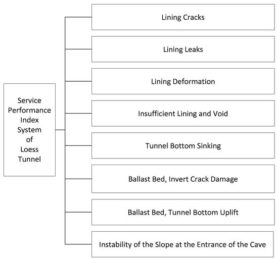
Figure 1.
Risk assessment indicators.
Taking lining leakage water as an example, we created a risk source classification diagram for lining leakage water diseases, as shown in Figure 2. Since the risk indicators of various disasters and accidents are repetitive to a certain extent, the risk sources of each disaster will not be listed one by one.
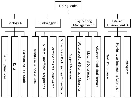
Figure 2.
Risk source classification diagram of water leakage disease.
3.2. Screening of Risk Indicators Based on the Improved TOPSIS Method
There are many factors affecting the service performance of tunnels. If each factor is studied and analyzed during evaluation, it will cause problems such as a complex model and a large amount of calculation. Therefore, it is advisable to select influential and representative factors for modeling [20,21]. Based on this, this paper uses the improved TOPSIS method to screen and sort complex factors, simplify the model, and reduce the amount of calculation.
The advantages of this method are as follows: Firstly, the method is simple, the structure is reasonable, the order is clear, and the application is flexible. Secondly, it makes full use of the original data information, and sorting results can quantitatively reflect the pros and cons of different evaluation objects, and it is intuitive and reliable. Thridly, there is no strict requirement for data (data distribution type, sample size, number of indicators are not strictly limited, suitable for small sample data, multi-unit evaluation, multi-index large system, suitable for continuous and dynamic data). Without reducing the number of variables in the calculation process, the original data can be directly used for calculation. Finally, the influence of different dimensions can be eliminated, so the evaluation indexes of different dimensions can be introduced at the same time for comprehensive evaluation.
Compared with the VIKOR (VIseKriterijumska Optimizacija I Kompromisno Resenje) method, TOPSIS is a set of distances based on the distance from the ideal solution. The VIKOR method proposes a compromise scheme with a dominant rate based on the TOPSIS method. The TOPSIS method considers not only the nearest distance to the positive ideal solution, but also the longest distance to the negative ideal solution, so as to determine the optimal solution and maximize the efficiency. In addition, the process of the TOPSIS method does not include any subjective factors, which is more suitable for a decision-making environment that requires completely objective results. Compared with the CRITIC (Criteria Importance Though Intercrieria Correlation) method, which loses some information due to the rank substitution of the index value, the TOPSIS method can make full use of the original data information.
Based on this, this paper uses the improved TOPSIS method to screen and sort complex factors, simplify the model, and reduce the amount of calculation.
- (1)
- Taking the risk probability, risk loss, and risk controllability as evaluation indicators, we constructed a decision matrix A according to the evaluation indicators:
- (2)
- Matrix normalization:
For positive indicators
For negative indicators
- (3)
- The ideal solution of the matrix. Solve for ideal values present in a normalized matrix:
Among them, J+ is a positive indicator, and J− is a negative indicator.
- (4)
- Euclidean weighted distance sum of squares. The weights corresponding to each index attribute are w1, w2,… wn, respectively, and the weighted sum of squared distances between the positive ideal value and the negative ideal value of each decision is:
Combined with the conditions of the tunnel project and the external environment, this paper uses the improved TOPSIS method to calculate the risk factors found in the process of the literature review and expert evaluation. Taking “external environment D” as an example, the underlying risk factors are identified and screened through calculation, and the ranking of risk factors is obtained.
D1 represnts earthquake, D2 represents the change in groundwater level, D3 represents external stacking, D4 represents train disturbance, D5 represents proximity engineering activity, and D6 represents the change in temperature and humidity. Taking D1–D6 as an example, the improved TOPSIS method is used to screen risk factors and the expert scoring method is used to assign weights to risk probability, risk loss, and risk controllability, and obtain the ranking of index factors. The calculation is as follows:
(1) Constructing the initial decision matrix: The initial indicator factor weights are shown in Table 1 below:

Table 1.
Initial risk factor indicators.
(2) Matrix normalization processing: risk probability and risk loss are negative indicators, risk controllability is a positive indicator. The data obtained from Formulas (8)–(11) are shown in Table 2.
Table 2.
Normalized risk factor index values.
(3) Calculation of weighted distance: the weights of risk probability W1, risk loss W2, and risk controllability W3 are determined by reviewing the literature and expert scoring, respectively, (0.315, 0.330, 0.355). From Formula (11) we get:
fD1(w) = 0.334, fD2(w) = 0.237, fD3(w) = 0.210,
fD4(w) = 0.226, fD5(w) = 0.252, fD6(w) = 0.270
(4) We sorted the weighted distance of the indicators to get:
fD1(w) > fD6(w) > fD5(w) > fD2(w) > fD4(w) > fD3(w)
We screened out risk indicators with smaller weighted distance values. In the same way, we identified and screened the underlying risk factors of geological landforms, hydrological conditions, and engineering management, and finally obtained 22 risk index factors.
4. Building a Bayesian Network Model
The first step is to classify the risk index factors in Table 3 that affect the service performance of the tunnel according to the catastrophic intensity. This model divides the indexes except “surrounding rock grade” into four grades. The surrounding rock grade is based on the BQ tunnel. The surrounding rock classification method is divided into five grades; the second step is to build an explanation structure model and divide the risk indicators into layers according to the relationship between them. The last step is to adjust and correct the causal relationship in the explanatory structural model according to the causal diagram method.
Table 3.
Risk indicator factors.
4.1. Explain the Construction of the Structural Model
ISM (interpretative structural modeling method) is an analysis method widely used in modern systems engineering. The essence of explaining the structural model is to give a simplified and hierarchical directed topology graph to the model system through a large number of mathematical topological operations [22,23].
Determine the influence diagram.
In the previous article, 23 input and output indicators were selected for tunnel service performance evaluation. The input indicators are shown in Table 3, and the output indicator is the tunnel service performance T. The influence diagram of each index is shown in Figure 3. In the figure, red indicates that the horizontal index has an impact on the vertical index, blue indicates that the vertical index has an impact on the horizontal index, yellow indicates that there is no mutual influence between the two indicators, and green indicates that there is mutual influence between the two indicators.
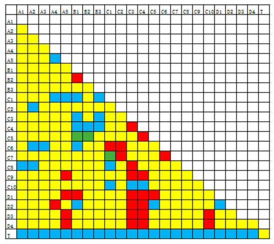
Figure 3.
Influence relationship of tunnel service.
Transform the adjacency matrix.
The adjacency matrix can further reflect the influence relationship between each index, and the transformation formula is as follows:
In the formula, aij represents the relationship between the index si and the index sj in the adjacency matrix. When a = 1, it means that the former has an influence on the latter, and when a = 0, it means no influence. The transformed adjacency matrix is shown in Equation (15).
Calculate the reachability matrix.
The reachability matrix G is mainly used to describe the reachable degree between each node in the network model after a certain length of path. The reachable matrix is obtained by continuous multiplication, and the calculation formula is as follows:
In Formula (15), n represents the number of iterative computations in the matrix A, and I represents the identity matrix. This operation can be realized by Boolean algebra operation in Matlab, and the calculated reachability matrix is shown in Equation (17).
Hierarchical processing.
In the reachability matrix G, the set composed of the indices corresponding to the column with a value of 1 in a single row becomes the reachable set L(Si), and the set composed of the indices corresponding to the row with a value of 1 in a single column can become the antecedent set Q(Si). The necessary and sufficient conditions for the variable set O1 to be the highest-level variable set are as follows:
The level division is shown in Table 4.
Table 4.
Hierarchical division table.
The calculated grading is slightly deviated from the actual situation. In order to make it closer to the actual engineering, the grading is adjusted. The adjusted grading is shown in Table 5.
Table 5.
Adjusted hierarchy division.
Establish an explanation structure model.
Figure 4 shows the loess railway tunnel service performance risk assessment and interpretation structure model established according to the adjusted hierarchical division table and the relationship between each index.
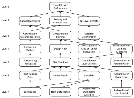
Figure 4.
Interpretation structure model of each index.
4.2. Correction of Causal Diagram Method
A causal diagram is a graph to describe the causal relationship between variables, focusing on the dependency between input and output [24,25,26,27,28,29,30,31,32,33]. Since the explanatory structural model may ignore the independence, direct, or indirect relationship among the indicators, the ISM model is further revised according to the causal diagram method, and a Bayesian network model finally suitable for the loess railway tunnel is obtained. The principle of correction of the cause-and-effect diagram method is as follows:
- (1)
- Check whether the indicators are independent. For example, the design defects in the construction management influencing factors may include excavation method selection defects and tunnel excavation cross-sectional area design problems, so arrows need to be added. The newly added arrows in Figure 5 are represented by dashed lines.
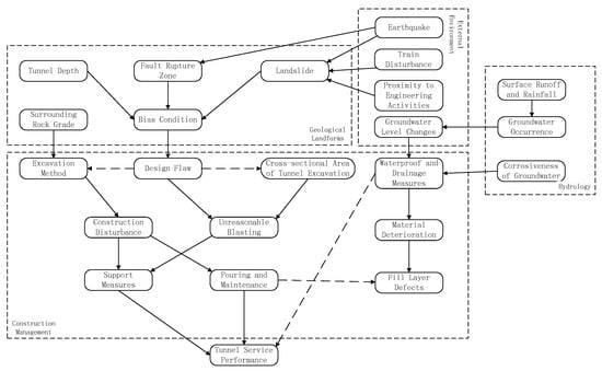 Figure 5. Bayesian network model of tunnel serviceability.
 - (2)
- Review the undiscovered direct or indirect relationship between the indicators. For example, the waterproof and drainage measures can affect the material condition and then cause the defect of the filling layer, which affects the service performance of the tunnel, but its direct influence on the service performance of the tunnel cannot be ignored, so it is necessary to add arrows between them to indicate this influence relationship.
- (3)
- Review the loop relationships in the network model. There is no loop relationship in Figure 5.
- (4)
- Review the causal inversion problem in the network model. There is no causal reversal in Figure 5.
5. Data Learning and Verification of Bayesian Network Model
Figure 5 shows the final Bayesian network model of tunnel service performance. In this paper, Netica software is used for data training, verification, and application, because the final result of the network output is the probability that the output index belongs to each classification interval. Therefore, first of all, it is necessary to classify each index to meet the input and output requirements of the network model; secondly, it is necessary to count engineering cases that can be applied to Bayesian network data training and verification and perform interval quantification processing, involving accuracy (ACC), precision (P), recall (R) and F1 value to evaluate the training effect of the model.
5.1. Determination of Input and Output Types of Each Evaluation Index
This model has a total of 23 indicators, of which 22 are input indicators and 1 is an output indicator. The catastrophic classification of each index has been completed in the previous section. Except for the “surrounding rock level”, the catastrophic levels of other input and output indicators are divided into four levels, and the “surrounding rock level” is divided into five levels. In the Bayesian computing software Netica, we compared the grading intervals of the indicators at all levels. English words that represent the degree of strength are used to express, let “strong” represent level I, “medium” represent level II, and “weak” represent level III, “none” indicates grade IV, and grade I is the most unfavorable condition. In the surrounding rock grades, “strong” represents the I-level surrounding rock, “medium1” represents the II-level surrounding rock, “medium2” represents the III-level surrounding rock, “weak” represents the IV-level surrounding rock, “none” represents the V-level surrounding rock, and level V is the most unfavorable situation.
5.2. Bayesian Network Model Training and Validation Results
This paper investigates a large number of cases of tunnel service performance failures and non-failures through a literature review and on-site visits. A total of 70% of the cases were selected to train the Bayesian network model, and 30% of the cases were used to verify the training results. Figure 6 shows the training results of the Bayesian network model of tunnel service performance.
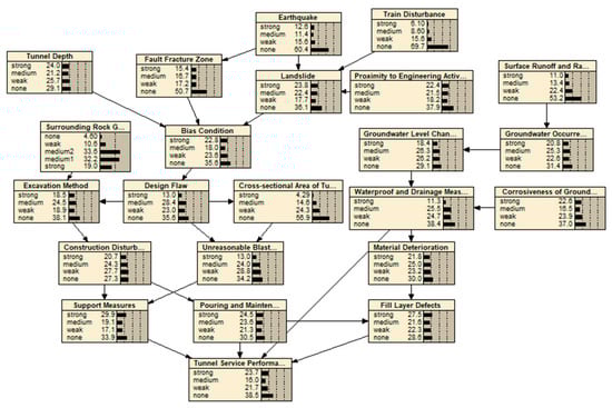
Figure 6.
Bayesian network training results.
The conditional probability of each indicator after Bayesian network model training is shown in Figure 6. The verification process of the model is to click the grading interval of each indicator to obtain the probability of belonging to the interval 100%, and then observe the probability of the output result.
Using 30% of the samples to verify the training results, the accuracy rate of the prediction results for the tunnel service performance reaches 92%, and the overall accuracy rate is high. The overall accuracy (ACC), precision (P), recall (R) and F1 value were introduced to comprehensively evaluate the training effect and prediction effect of the model. Its calculation formula and corresponding confusion matrix are as follows:
In the formula, the accuracy rate P represents the precision of the prediction result; the recall rate R represents the correct degree of the positive example in the result being predicted; and F1 is the compromise between the two, which can reflect the prediction effect of the network more comprehensively. When the range of F1 is 0–1 and the value is higher, it indicates that the network prediction result is more accurate. In Table 6, true and false of the true value represent whether the tunnel service performance fails in the actual case; true and false of the predicted value represent that the predicted result is failure occurred or not; and true positive (TP) represents the failure of the case where the failure occurred. The prediction result is also the occurrence of failure. Similarly, the interpretation of false negative (FN), false positive (FP), and true negative (TN) can be applied. The confusion matrices of the predicted tunnel service performance are shown in Table 6 and Table 7, respectively.
Table 6.
Confusion matrix.
Table 7.
Confusion matrix of tunnel service performance.
The prediction results of the model for the service performance of tunnels are as follows. For the two categories of strong and none, the accuracy rate P is 100%, the recall rate R is 100%, and the F1 value is 1. For the category medium, the accuracy rate P is 80%, the recall rate R is 100%, and the F1 value is 0.89. For the overall prediction result of tunnel service performance, the overall accuracy ACC is 92%.
For multi-class problems, the overall accuracy is only one, similar to how it is calculated for two-class problems. For precision and recall for a multi-class confusion matrix, any value on the symmetry axis of a skew symmetric matrix divided by the sum of the rows is the precision and divided by the sum of the columns is the recall. The calculation method of the F1 value is consistent with Equation (22). From the overall verification results of the model, the overall accuracy has reached more than 90%, and the accuracy is high, which can meet the engineering application. For service performance prediction, there is only a small amount of error between the predicted value and the actual case. The error is only a judgment error of adjacent categories, and there is no cross-level prediction error, mainly due to the lack of overall samples. With the gradual development of subsequent sample databases abundant, the statistics of each evaluation index are sound, and the prediction error will be gradually reduced.
6. Applications of Bayesian Network Models
This paper selects the K1759 + 135~K1761 + 030 section of the Zhangjiazhuang tunnel on the Lanxin high-speed railway to further verify the feasibility of the model and introduces the application method of the model in detail.
6.1. Engineering Background
The Zhangjiazhuang tunnel on the Lanxin high-speed railway is located in Honghui Town, Ledu District, Haidong City, Qinghai Province. It is a single-hole, double-track railway tunnel with a buried depth of 50–290 m. The Zhangjiazhuang tunnel passes through the Qilian Mountains, the terrain is undulating, the ground elevation is between 1850 and 2300 m, and the loess gullies are developed, mostly in a “V” shape, with little vegetation coverage on the mountains. There are many earthquakes with high frequency and high intensity. Since 1900, there have been 17 strong earthquakes of magnitude 6.5 or above in Qinghai, including 5 earthquakes of magnitude above 7, and the largest earthquake with a magnitude of 8.1. The basic meteorological characteristics are high cold, drought, long sunshine time, large temperature difference between day and night, small temperature difference between winter and summer, large difference in climate and geographical distribution, temperature decreases with the increase in altitude, and rainfall increases with the increase in altitude. The annual average temperature is 3.2–8.6 °C, and the average annual rainfall is 319.2–531.9 mm, mostly concentrated between July and September. The section K1759 + 135~K1761 + 030 of the tunnel is 1895 m long and has grade IV surrounding rock.
In January 2016, a geological disaster occurred in Zhangjiazhuang tunnel. There were cracks on the right side of the vault of the K1759 + 139~K1759 + 145 section of the tunnel, and the crack width was approximately five millimeters. There were two concrete peeling blocks and block drops. The K1759 + 145~K1759 + 151 arch wall had longitudinal cracks, and the maximum crack width was approximately 10 mm. The K1759 + 606 right arch wall construction joint concrete spalling of approximately 1 m2. The K1759 + 618~K1759 + 666 section right part of the concrete in the side arch part fell off, with a maximum falling range of approximately four meters. The two catenary suspenders located at K1759 + 626 and K1759 + 648 fell off. The ballastless track in the tunnel was also displaced accordingly, and the line was forced to suspend operation. The disease detection situation of the Zhangjiazhuang tunnel is shown in Figure 7. According to the summary of engineering data, this paper intends to use the built Bayesian network model to evaluate the service performance of the Zhangjiazhuang tunnel K1759 + 135~K1761 + 030 under no rain and heavy rain.
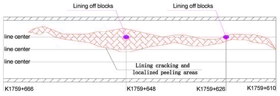
Figure 7.
Zhangjiazhuang tunnel disease detection.
6.2. The Influence of Rainfall on the Service Performance of the Tunnel
This is based on the previously built and verified Bayesian network model, as shown in Figure 6. We entered the index value information into Table 8 in turn, and observed whether the final output result was consistent with the actual situation. Figure 8 and Figure 9 show the prediction results of the service performance of sections K1759 + 135~K1761 + 030 of the Zhangjiazhuang tunnel under the conditions of no rain and heavy rain, respectively. The method for determining the index level is to click the corresponding level of the index in turn in the software operation interface, so that the probability of belonging to the interval is 100%.
Table 8.
Overview of the values of input indicators for rainfall and non-rainfall.
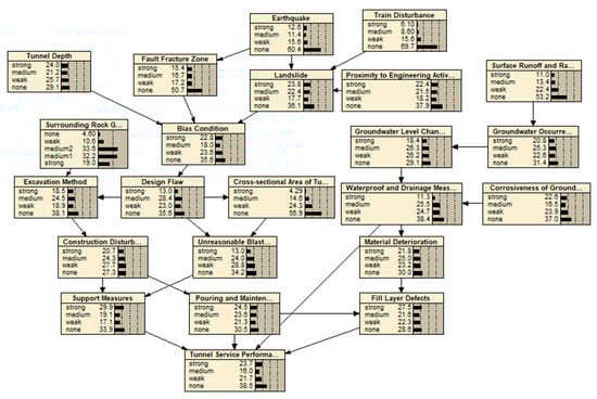
Figure 8.
Prediction results of the no-rain model.
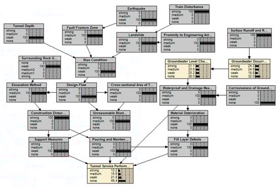
Figure 9.
Prediction results of the rainfall model.
According to the final output results, it is found that the prediction results of the service performance of the tunnel section are basically consistent with the actual conditions under the conditions of rain and no rainfall. This model is more accurate and more practical for the prediction of tunnel service performance under rainfall conditions.
7. Conclusions and Future
Based on the Bayesian network, this paper used Netica software to establish an evaluation model for the service performance of loess railway tunnels in a broad sense. Based on the improved TOPSIS method, the screening of many complex risk factors was completed, the representative evaluation indexes of tunnel service performance were selected, and the input and output indexes were classified. Through the ISM model and causality diagram correction method to determine the relationship between the nodes, we established a Bayesian network evaluation model. The EM algorithm is used for network training, and the network training results are evaluated by overall accuracy (ACC), accuracy (P), recall rate (R) and F1 value. The evaluation results show that the accuracy of the model is high, reaching more than 90 %. It can be seen that this model improves the ability of the Bayesian network to solve uncertain problems. The application results of engineering examples show that this method can accurately evaluate the service performance of tunnels and is also applicable in the case of incomplete index statistics. It can be used as a decision-making tool for risk analysis of tunnel service performance.
Limited by the actual situation of the project and the author’s limited abilities, there are still many problems and shortcomings to be further studied. Firstly, a more detailed classification of risk indicators in required to improve the degree of quantification. The classification of risk indicators in this paper can basically achieve the conversion between qualitative analysis and quantitative analysis; however, a larger dataset will make the training results have a certain error and will increase the level of indicators to further improve the accuracy of the assessment. Secondly, more tunnel damage sections are selected for serviceability assessment to obtain the influence mechanism of single factor or even multi-factor combinations on tunnel service performance.
Author Contributions
Conceptualization, Y.Y.; data curation, F.X., M.D. and L.H. (Linyan Hou); writing—review & editing, Q.Z. and L.H. (Lili Hou). All authors have read and agreed to the published version of the manuscript.
Funding
This research was funded by the national key R&D program of China, grant number 2018YFB1600200; the NSFC high-speed railway joint fund, grant number U2034207; and the Natural Science Foundation of Hebei Province, grant number E2022210065. This paper was funded by the China scholarship council.
Data Availability Statement
Not applicable.
Acknowledgments
We would like to thank the anonymous referees for their helpful comments and suggestions.
Conflicts of Interest
The authors declare no conflict of interest.
References
- Chen, Z.; Yue, H. Construction Technology of Water and Mud Inrush Treatment in Loess Tunnel. Railw. Eng. 2011, 5, 77–79. [Google Scholar]
- Zhang, X.; Bi, H.; Xia, W. Experimental Study on Surface Precipitation of Yima No.1 Water-rich Loess Tunnel Construction in Yinchuan–Xi’an High Speed Railway. Railw. Eng. 2018, 58, 91–94. [Google Scholar]
- Li, M.; Pan, C.; Zhang, X. Research on Fluid-Structure Interaction Mechanism by The Large Section Tunnel in Loess Strata with Rich Water of Lanzhou Subway. Highway 2018, 63, 323–327. [Google Scholar]
- Su, Q. Study on Safety Risk Assessment and Countermeasures for Portal Excavation of Collapsible Loess Tunnel; Lanzhou Jiaotong University: Lanzhou, China, 2020. [Google Scholar]
- Bai, W.; Li, R.; Zhao, X.; Liu, J.; Zou, Z. Based on Loess Arch Sliding Line Field Visualization Program Design and Parameter Sensitivity Analysis. J. Disaster Prev. Mitig. Eng. 2020, 40, 132–138. [Google Scholar]
- Wei, R. Study on The Formation Mechanism and Control Technology of Seepage Disease in The Lishi Loess Tunnels of Li-Jun Expressway; Xi’an University of Science and Technology: Xi’an, China, 2017. [Google Scholar]
- Guo, S. Study on Mechanism and Countermeasoure of Large Deformation of Deep Buried Old Loess Tunnel; Southwest Jiaotong University: Chengdu, China, 2017. [Google Scholar]
- Yan, Q. Research on Numerical Simulation Method for Large Deformation Evolution of Loess Tunnel and Its Supporting Mechanical Behavior; Shandong University: Jinan, China, 2018. [Google Scholar]
- Ling, Y.; Zhao, Y.; Miao, X. Analysis of Characteristics and Formation Mechanism of Ground Surface Cracks of Shallow Buried Loess Tunnel with Large Section. Railw. Stand. Des. 2020, 64, 115–120. [Google Scholar]
- Wang, J.; Wang, D. Study on Time-dependent Reliability of In-service Tunnel Structure under Multiple Failure Modes. Railw. Stand. Des. 2019, 63, 91–96. [Google Scholar]
- Guo, J.; Yang, Z.; Kang, F. Analysis of Deformation Stability Reliability of Tunnel Surrounding Rocks Based on Vector Projection Response Surface Method. Mod. Tunn. Technol. 2019, 56, 70–77. [Google Scholar]
- Yang, J.; Shen, K.; Shu, L.; Xue, Y.; Wang, J. Risk Mechanism and Assessment of Large Deformation in Soft Rock Tunnel. J. Railw. Eng. 2022, 39, 81–86. [Google Scholar]
- Tang, Y. Research on Risk Assessment and Management Methods for Projects of Railway Tunnels Passing under Expressways. Mod. Tunn. Technol. 2022, 59, 220–226. [Google Scholar]
- An, Y.; Li, J.; Zhao, D.; Zhang, Y.; Yang, G. Comprehensive extension assessment on tunnel structure health. J. Railw. Sci. Eng. 2020, 17, 422–428. [Google Scholar]
- Yin, R. Fuzzy Stochastic Reliability Analysis of Serviceability Limit State for Linings of Operating Highway Tunnels. China Civ. Eng. J. 2016, 49, 122–128. [Google Scholar]
- Zhang, J.; Wei, K.; Qin, S. A Bayesian Updating Based Probabilistic Model for The Dynamic Response of Deepwater Bridge Piers under Wave Loading. Eng. Mech. 2018, 35, 138–143+171. [Google Scholar]
- Guo, F.; Wang, H. Risk Assessment of Tunnel Construction by Using Fuzzy Comprehensive Evaluation Method Based on Bayesian Networks. J. Railw. Sci. Eng. 2016, 13, 401–406. [Google Scholar]
- Zhang, W.; Jiang, Y.; Yin, G.; Lean, Y. Handling Missing Values in Software Effort Data Based on Naive Bayes and EM Algorithm. Syst. Eng.-Theory Pract. 2017, 37, 2965–2974. [Google Scholar]
- Yu, K.; Wang, H.; Wu, X.; Yao, H. Learning Bayesial Networks Using A Parallel EM Roach. Res. Appl. 2008, 21, 670–676. [Google Scholar]
- Chen, J.; Zhou, F.; Yang, J.; Liu, B. Fuzzy Analytic Hierarchy Process for Risk Evaluation of Collapse During Construction of Mountain Tunnel. Rock Soil Mech. 2009, 30, 2365–2370. [Google Scholar]
- Tian, R.; Meng, H.; Chen, S.; Wang, C.; Sun, D.; Shi, L. Prediction of Intensity Classification of Rockburst Based on Deep Neural Network. J. China Coal Soc. 2020, 45, 191–201. [Google Scholar]
- Fang, D.; Zhang, Z.; Yin, Y. Research on Interpretative Structural Model for Operational Risk System of Tunnel. J. Wuhan Univ. Technol. 2010, 32, 164–168. [Google Scholar]
- Li, C. Risk Assessment and Warning Research of Water Inrush in Karst Tunnels Based on Data Learning; China University of Mining and Technology: Xuzhou, China, 2020. [Google Scholar]
- Yang, X. Subway Operation Risk Assessment Based on Fuzzy ISM Model and FMICMAC Model; Southwest Jiaotong University: Chengdu, China, 2019. [Google Scholar]
- Li, X.; Zhang, C.; Yuan, D. An in-tunnel jacking above tunnel protection methodology for excavating a tunnel under a tunnel in service. Tunn. Undergr. Space Technol. 2013, 34, 22–37. [Google Scholar] [CrossRef]
- Špačková, O.; Straub, D. Dynamic Bayesian network for probabilistic modeling of tunnel excavation processes. Comput.-Aided Civ. Infrastruct. Eng. 2013, 28, 1–21. [Google Scholar] [CrossRef]
- Sousa, R.L.; Einstein, H.H. Risk analysis during tunnel construction using Bayesian Networks: Porto Metro case study. Tunn. Undergr. Space Technol. 2012, 27, 86–100. [Google Scholar] [CrossRef]
- Zhang, L.; Wu, X.; Qin, Y.; Skibniewski, M.J.; Liu, W. Towards a fuzzy Bayesian network based approach for safety risk analysis of tunnel-induced pipeline damage. Risk Anal. 2016, 36, 278–301. [Google Scholar] [CrossRef] [PubMed]
- Balta, G.C.K.; Dikmen, I.; Birgonul, M.T. Bayesian network based decision support for predicting and mitigating delay risk in TBM tunnel projects. Autom. Constr. 2021, 129, 103819. [Google Scholar] [CrossRef]
- Zhao, Y.; He, H.; Li, P. Key techniques for the construction of high-speed railway large-section loess tunnels. Engineering 2018, 4, 254–259. [Google Scholar] [CrossRef]
- Xue, Y.; Zhang, X.; Li, S.; Qiu, D.; Su, M.; Li, L.; Li, Z.; Tao, Y. Analysis of factors influencing tunnel deformation in loess deposits by data mining: A deformation prediction model. Eng. Geol. 2018, 232, 94–103. [Google Scholar] [CrossRef]
- Xu, Z.; Cai, N.; Li, X.; Xian, M.; Dong, T. Risk assessment of loess tunnel collapse during construction based on an attribute recognition model. Bull. Eng. Geol. Environ. 2021, 80, 6205–6220. [Google Scholar] [CrossRef]
- Shao, S.J.; Deng, G.H. Strength Characteristic of Loess with Different Structure and Its Application to Analyzing Earth Pressure of Loess Tunnel. In Boundaries of Rock Mechanics; CRC Press: Boca Raton, FL, USA, 2008; pp. 541–546. [Google Scholar]
Disclaimer/Publisher’s Note: The statements, opinions and data contained in all publications are solely those of the individual author(s) and contributor(s) and not of MDPI and/or the editor(s). MDPI and/or the editor(s) disclaim responsibility for any injury to people or property resulting from any ideas, methods, instructions or products referred to in the content. |
© 2023 by the authors. Licensee MDPI, Basel, Switzerland. This article is an open access article distributed under the terms and conditions of the Creative Commons Attribution (CC BY) license (https://creativecommons.org/licenses/by/4.0/).