Predicting Model Training Time to Optimize Distributed Machine Learning Applications

Abstract

Despite major advances in recent years, the field of Machine Learning continues to face research and technical challenges. Mostly, these stem from big data and streaming data, which require models to be frequently updated or re-trained, at the expense of significant computational resources. One solution is the use of distributed learning algorithms, which can learn in a distributed manner, from distributed datasets. In this paper, we describe CEDEs—a distributed learning system in which models are heterogeneous distributed Ensembles, i.e., complex models constituted by different base models, trained with different and distributed subsets of data. Specifically, we address the issue of predicting the training time of a given model, given its characteristics and the characteristics of the data. Given that the creation of an Ensemble may imply the training of hundreds of base models, information about the predicted duration of each of these individual tasks is paramount for an efficient management of the cluster’s computational resources and for minimizing makespan, i.e., the time it takes to train the whole Ensemble. Results show that the proposed approach is able to predict the training time of Decision Trees with an average error of 0.103 s, and the training time of Neural Networks with an average error of 21.263 s. We also show how results depend significantly on the hyperparameters of the model and on the characteristics of the input data.

1. Introduction

Despite the significant advances that the field of Machine Learning (ML) has seen in recent years, there are still scientific and technical challenges to solve [1]. These stem from many different factors including the volume of the data [2], streaming data [3], low-quality and diverse data [4], or Ethical requirements, just to name a few. Thus, new developments are expected to address these challenges in the coming years, which currently makes the field of ML an exciting field of interdisciplinary research.

One of the shifts that occurred in recent years to address these challenges, namely the size of the data, was to move towards a distributed paradigm, in terms of storage, model training, and model serving [5]. Obviously, this brings along new challenges, namely in what pertains to task and algorithm distribution and allocation, or coordination.

At the same time, new environmental guidelines and legislation push towards a more efficient management of data clusters [6]. Nowadays, brute-force or exhaustive approaches to ML are no longer desirable either because they require too many computational resources or because the time they take is just too long due to the size of the data.

This work is thus motivated by the challenge of devising more efficient distributed ML environments, that provide the cluster with better means to manage the underlying services. Namely, we seek to find better ways to scale and assign ML tasks (model training and prediction) across the cluster, with the goal of having the best models (accuracy) while minimizing resources consumption (efficiency).

The proposed approach emerged in the context of the Continuously Evolving Distributed Ensembles (https://ciicesi.estg.ipp.pt/project/cedes (accessed on 3 February 2023)) (CEDEs) project and implements the possibility of predicting the training time of a given ML model. In a distributed learning scenario, in which dozens or hundreds of tasks may have to be coordinated in a given time, having a prediction of their cost (time) is paramount to better distribute them.

While this task is generic and applicable to any ML setting, we frame it in the context of the CEDEs project. However, the same methodology could be used in any other domain to achieve similar purposes.

The main goal of this work is thus to determine whether the proposed approach, which relies on meta-learning, can be used to develop models that accurately predict the training time of ML models. The secondary goal is to determine which factors significantly influence this. Model hyperparameters [7] are investigated first, as the relationship between these and training time is often obvious. We aim not only to identify them but to model their influence on training time. Next, we also investigate whether the features about the data are relevant [8]. That is, would the same algorithm, with the same configuration, applied to the same amount of data have different training times if these sets of data had different characteristics?

By characteristics we refer to meta-features, that is, features that describe the properties of datasets. These can include statistical properties, measures of entropy or data quality, shape of the dataset (e.g., row-to-column ratio), distribution of the data and relationships to the dependent variable, among many others [8].

The achievement of this goal opens the door to the development of a better way to plan and distribute ML tasks, especially in a distributed scenario. Specifically, two main contributions of this work can be pointed out. First, we show that the training time of a model depends significantly on the type of algorithm used, as well as on the specific hyperparameters set. Second, we show that the actual characteristics of the input data (the meta-features) are also relevant. By combining these factors, we are able to reliably predict the training time of a model, which will then be used by the optimization module for distributed task allocation.

The rest of the paper is structured as follows. Section 2 presents the related work, and Section 3 provides some background on the main topics addressed in this work, namely, Distributed Learning, Meta-Learning and Optimization. Next, Section 4 describes project CEDEs which is both the motivation and the use case for this work. Specifically, it discusses the relevance of the problem addressed. The methodology followed is detailed in Section 5, followed by an analysis and discussion of the results, respectively, in Section 6 and Section 7. The paper ends with a summary of the main findings and conclusions in Section 8.

2. Related Work

The advancement of the ML field has led to a growing need for high-computing resources during the training of models, as large amounts of data are utilized. Despite this, many researchers in the field focus primarily on the development of high-accuracy models, neglecting the computational cost as a crucial factor [6]. However, there are a number of techniques available to evaluate or estimate the computational cost of ML applications.

This section examines the various techniques for predicting the use of computing resources in ML applications, including their respective advantages and disadvantages, summarized in

Table 1. Advantages and disadvantages of the main techniques for estimating algorithm training time.

Technique	Advantages	Disadvantages
PMC	No overhead, application-independent	No pre-processor results
Simulation	Detailed results	Significant overhead
Real-time	Easily available	Not generalizable

. It also establishes connections between these approaches and the implementation of similar techniques in the CEDEs project.

One such approach uses regression and correlation techniques to predict the power consumption of a system based on the values of the performance counters (PMCs) [6,9,10,11,12,13,14,15,16]. The approach typically involves collecting data on the values of the performance counters while the system is running and then using this data to train a regression or correlation model. This model can then be used to predict the power consumption of the system for a given set of input data. This approach can be used to evaluate the computational cost of a ML application and to identify the factors that are most important for performance.

Other approaches rely on simulation using parametrized power models and analytical dynamic power equations to estimate power values [6,17,18,19,20]. Parametrized power models are mathematical equations that describe the relationship between power consumption and various system parameters, such as the number of transistors, the clock frequency, or the voltage. These models can be derived from experimental data or from measurements of actual systems.

Analytical dynamic power equations are mathematical expressions that describe the power consumption of a system over time, based on the dynamic behaviour of the system. These equations take into account factors such as the switching activity of the transistors and the capacitance of the interconnects.

These power equations can be used to estimate the power consumption of a system for a given set of input data, such as clock frequency, voltage, and temperature. This approach can be used to evaluate the computational cost of a ML application and to identify the factors that are most important for performance.

Another type of approach relies on real-time power estimation [6,9,10,11,12,13,14,15,16,21,22], which refers to the process of measuring the power consumption of a system in real-time, as the system is running. This is typically done by measuring the voltage and current flowing through the system, and then using these measurements to calculate power consumption. The measurement can be done using specialized power measurement hardware or software tools.

Most of the existing work, as this analysis shows, is devoted to measuring computational resources, which do not translate directly to training time. In fact, to the best of our knowledge, at the time of writing this document, this issue was only addressed in [23]. However, the work of [23] has some differences compared to the approach described in this paper. First, it is specific to recommendation systems. Second, it requires a sample of the dataset, to provide an estimate of the training time over the complete dataset. Finally, it is not suitable to be used in a distributed learning setting, such as that of CEDEs.

The approach that has been implemented in the CEDEs project is to collect specific metadata, such as CPU and memory usage, the queue of tasks on the node where the training process is being performed, the number of blocks, the algorithms used, and specific configuration parameters. These collected data can then be used as input to a regression model, which can predict the training time of the base model with a high degree of accuracy.

Despite the lack of research and focus on this topic, it is clear that the techniques mentioned above have similarities with the approach presented in the CEDEs project. In most cases, there is a data collection process and a mathematical function is applied to those metrics in order to obtain an estimate of the value to be analyzed. The study conducted in this field was very useful for this project, as an estimate of the training time of a model not only provides greater control over the application, but also helps the optimization module to more efficiently choose which node to assign the next tasks to and ultimately aid in reducing the consumption of computational resources.

3. Background

This section provides some relevant background on the main topics addressed in this paper, namely, Distributed Learning, Meta-Learning and Optimization.

3.1. Distributed Learning

ML systems gained an unprecedented relevance in recent years. In addition, as the demand for ML grows, so does the complexity of developing ML systems [24].

The criteria for training a big ML model can no longer be met by a single device or laptop. For example, when the computational complexity of the method exceeds the main memory, the algorithm will not scale well due to memory constraints, highlighting the scalability and efficiency limitations of ML algorithms.

The size and availability of training datasets for ML tasks have skyrocketed as a result of the disruptive trend towards big data. On a single GPU, converging such models on large datasets could potentially take weeks or even months [24,25].

As a consequence, ML researchers and data analysts need to develop programs that can operate on multiple machines and be accessed by users from all over the world in order to train a large ML model with a significantly larger amount of data.

Due to the increasing complexity and demand ML systems, in order to be competitive, these must be designed to handle the unprecedentedly growing scale, such as the growing volume of historical data, the frequent batches of incoming data, the complex ML architectures, the heavy model-serving traffic, the intricate end-to-end ML pipeline, the user demands for faster responses to satisfy practical requirements, etc [24,25]. In these cases, distributed ML algorithms may be considered.

Before the invention of distributed frameworks, users had to develop hard-coded solutions, explicitly controlling each part of the execution on their own. This time-consuming and error-prone procedure involved handling data distribution, parallelization, synchronization, and fault tolerance. This prolonged the development cycle and made it challenging for users to implement new algorithms and troubleshoot current ones [26].

Computer programs now run on several machines instead of just being able to execute on one. The creation of large-scale data centers, which include hundreds or thousands of computers that communicate with one another via a shared network, has helped in meeting the rising demand for computing and the pursuit of higher efficiency, reliability, and scalability [24].

A distributed system, to put it simply, is a system whose components are distributed over various networked computers that communicate with each other to coordinate tasks and collaborate via message passing.

Likewise, distributed ML is a multi-node ML system that improves performance, increases accuracy, and scales to larger input spaces. A distributed ML system is composed of a pipeline of operations and components that handle various ML application functions, including data ingestion, model training, model serving, etc. [24].

By parallelizing over a large number of machines, the system is more scalable and reliable when handling large-scale problems (e.g., large datasets, large models, heavy model-serving traffic, and complicated model selection or architecture optimization) [24]. This enables a model to train larger models on more data faster, enabling producing higher quality models with faster iteration cycles [24]. Additionally, it minimizes computer errors and helps people interpret and draw conclusions from vast amounts of data.

Deep Neural Networks can be trained using one of two basic paradigms: model-parallelism, where the model is distributed, and data-parallelism, where the data is distributed.

Model-parallelism describes a situation in which each machine only possesses a portion of the model, such as a few layers of a deep Neural Network (referred to as “vertical” partitioning) or a few neurons from the same layer (referred to as “horizontal” partitioning).

Data-parallelism is the process of running a forward and backward pass over the local batch of data on each machine while maintaining a complete copy of the model. This paradigm scales more effectively by definition, since there is a capability to always add more machines to the cluster by either maintaining a constant global batch size (cluster-wide) while reducing the local batch size (per machine), or by maintaining a constant local batch size while increasing the global batch size. In data parallelism, the global batch size grows linearly with the cluster size. In practice, this scaling behaviour enables training models with extremely large batch sizes that would be impossible on a single machine because of its memory limitations. There is nothing preventing from distributing both the model and the data over the cluster, demonstrating the fact that the parallelism of the model and the data are not mutually exclusive but rather complementary.

Hyperparameter-parallelism is the last option, in which the same model is run on the same data using different hyperparameters on each computer.

Utilizing distributed learning has a number of inherent advantages, such as being more failure tolerant than isolated ML systems. If an organization has eight separate data streams in different machines spread across two data centers, it will function normally, even if one of the data centers fails. As a result, reliability is increased since when one model, machine or stream malfunctions, the entire system does too. However, distributed systems continue to function even when one or more models or data centers go down.

The time required to solve complex problems can also be reduced by using distributed learning to divide them into smaller chunks and handle them on a number of computers in parallel.

Given that they operate across multiple machines, distributed learning systems are inherently scalable. So, a user can install additional nodes to meet the increased load rather than continually updating a single system. Each cluster in a system can work to its full potential when under intense strain, and some clusters can be turned off when the load is low.

Finally, distributed ML systems are significantly more cost-effective than large centralized systems. Although they initially cost more than centralized systems, they scale more affordably after a certain point.

3.2. Meta-Learning

Machine Learning has been used by a wide range of businesses in recent years due to its ability to accelerate corporate operations, reduce costs, and provide better customer service [27].

Determining which of the many available algorithms is best suited to handle a certain problem is one of the many open challenges that remain to be addressed [28].

A potential solution to this issue is meta-learning, which may be used to automate the implementation and maintenance of a ML system within an organization or, at the very least, aid in the adoption of ML in businesses that cannot afford to hire specialized ML experts.

It can also be helpful for both beginners and experienced data scientists. The enormous and ongoing growth of data and the requirement to retrain or update models [29], or propose an alternative algorithm to handle the new data, present data scientists with yet another problem. Both of these issues can be solved via the use of meta-learning.

Meta-learning can generally be described as the ability of learning to learn [30]. To do this, it makes use of meta-data with the intention of discovering more about the data itself. It is based on meta-features, which are comparable to hyperparameters (parameters whose values are used to regulate the learning process in an ML model [31,32]) and which, in the context of meta-learning, describe the original data source.

In general, these meta-features can be divided into three categories: (i) features that characterize the properties of the original dataset, (ii) interactions between the attributes, and (iii) correlations between the attributes and the target column.

These features can be as basic as the number and distribution of classes, or as sophisticated as statistical data (such as mean kurtosis of attributes, mean skewness, etc.), information-theoretic properties (such as noise signal ratio, class entropy, etc.), among other measures. Systems that use meta-learning are currently being developed, and this is a field that is continuously expanding over time [33].

The term meta-dataset refers to a dataset that describes the features of other data, a dataset that includes meta-features. In contrast, a model that was developed using such data is known as a meta-model, while meta-learning has a wide range of applications, in this work it is explored to estimate the training time of a specific ML model, based on data about many past ML experiments.

3.3. Optimization

Optimization problems can be represented through mathematical models representing the problem objective, resources, constraints and decision variables. Optimization can be then stated as, the process of determining the value for the decision variables that allows the best possible result to be reached taking into account the resources and constraints imposed by the model. The practical applicability of optimization problems is quite evident in our daily life, such as route planning, production planning, packaging and packing, and image processing, among others. Due to the importance of these problems in several areas, the implementation of algorithms that obtain high-quality results in acceptable computational times has been the target of increasing research. Solution methods for solving those problems can be divided into two categories: exact and non-exact methods.

Exact methods guarantee the obtaining of the optimal solution for any instance of a problem, usually at the cost of high computational resources, even for small and medium-sized instances. The search for the optimal solution is done through the enumeration of the whole solution space. Among the most commonly used exact methods, we refer to Branch-and-Bound [34] and Dynamic Programming [35]. Branch-and-Bound implicitly enumerates all possible solutions to the problem under consideration by storing partial solutions (sub-problems) in a tree structure. There are initial considerations that can have a significant impact on the performance of these algorithms, namely, the search strategy (order in which the sub-problems in the tree are explored, e.g., Depth First Search), the branching strategy (how the solution space is partitioned to produce new sub-problems in the tree, e.g., binary), and the pruning strategy (definition of rules to prevent the exploration of sub-optimal regions of the tree). Dynamic programming solves optimization problems by dividing them into simpler sub-problems and taking advantage of the fact that the optimal solution to the global problem depends on the optimal solution of its sub-problems.

On the other side, non-exact methods, such as heuristics, do not guarantee that the optimal solution is obtained, but usually they provide very good approximations with fewer computational resources. Heuristics are problem-specific solution methods and are commonly divided into three categories: constructive, local search, and metaheuristic-based heuristics.

A constructive heuristic starts with an empty solution and iteratively creates a new solution following some rules, e.g., adding one element at a time to the current solution given a sequence of elements. Local search heuristics (see Yagiura and Ibaraki [36]) iteratively explore the neighbourhood (set of solutions that is possible to reach by means of a move specific to the neighbourhood structure applied) of the current solution to find a better one. The main disadvantage of the local search is its inability to escape local optima (which may or may not be the global optimum), as the search ends when it fails to improve the current solution with the chosen neighbourhood structure. Metaheuristics are general methodologies for solving problems that are adaptable to specific problems and can explore the solution space more efficiently as they promote the correct balance between intensification (deeper exploration of neighbourhoods considered promising) and diversification (exploration of less attractive neighbourhoods to escape local optima).

The Greedy Randomized Adaptive Search Procedure (GRASP) [37], Tabu Search [38], Path Relinking [39], Variable Neighbourhood Search (VNS) [40], Genetic Algorithms [41] and Scatter Search [39] are some of the most popular metaheuristics. The GRASP metaheuristic is a multi-start method with two phases. The construction phase builds a solution through partial randomisation of a greedy heuristic, while the local search phase improves the solution by means of a local search method. This process is repeated until a stopping criterion is reached, such as the maximum number of solutions generated. The Tabu Search extends local search allowing the exploration of solution space regions that are not considered promising, i.e., allowing to move to a solution that is worse than the current if no better solution is found. This metaheuristic makes use of memory structures to guide the search, e.g., to discourage revisiting already explored search spaces. The Path Relinking incorporates into a solution (i.e., initializer) attributes from another solution (i.e., guiding) exploiting the trajectories connecting them, while VNS combines local search with the dynamic change of neighbourhoods to escape the local optimums. Genetic Algorithms are probabilistic search methods inspired by the principles of natural selection and genetics to obtain individuals well adapted to their environment. In this metaheuristic, a population of solutions to a problem is evolved over multiple generations (until a stopping criterion is met, e.g., number of generations). There are two important decisions required to apply a Genetic Algorithm to a problem, namely, the representation of the solution (as a chromosome to represent an individual), and the definition of the fitness function to measure the quality of the chromosome. The fittest individuals of a particular generation are selected (see [42] for a review of selection methods) to serve as progenitors of the individuals of the next generation. New chromosomes are created by combining genetic operators: crossover (combination of progenitors to create a new chromosome) and mutation (random change of chromosomes for diversification). The Scatter Search is an evolutionary method in which a population of solutions evolves with the combination of its elements. This metaheuristic builds new solutions from the combination of solutions belonging to a reference set that contains high-quality and diversified solutions to allow intensification and diversification in the search.

Many more metaheuristics have been proposed to solve optimization problems, and we refer to [43] for a comprehensive historical perspective and to [44,45] for various classifications of metaheuristics, as they can be classified according to various criteria; for example, Genetic Algorithms could be classified as population-based (since they consider the crossover of multiple solutions through generations) and nature-inspired approach, while Tabu Search could be classified as a trajectory-based and nonnature-inspired approach.

Optimization is prescriptive by nature, while ML has a broader decision scope depending on the type of application: it can be descriptive (using unsupervised learning), predictive (using supervised learning), and prescriptive (using reinforcement learning). Taking advantage of each other strengths, one area of research that has gained traction in recent years is the hybridization of Optimization and ML. For example, ML can be used in Optimization methods helping search procedures, estimating evaluation functions or selecting algorithms considering the data characteristics or previous knowledge. Optimization, on the other side, can be used, for example, to optimize ML parameters and hyperparameters. We refer the interested reader in Optimization and ML hybridization to [46,47,48].

4. The CEDEs Project as a Use Case

This paper addresses the problem of predicting the training time of a ML model, and of analyzing the underlying relevant factors, while this problem is relevant in any ML setting, especially those in which big data and/or streaming data exist, the motivation for the work arose from the CEDEs project (Figure 1).

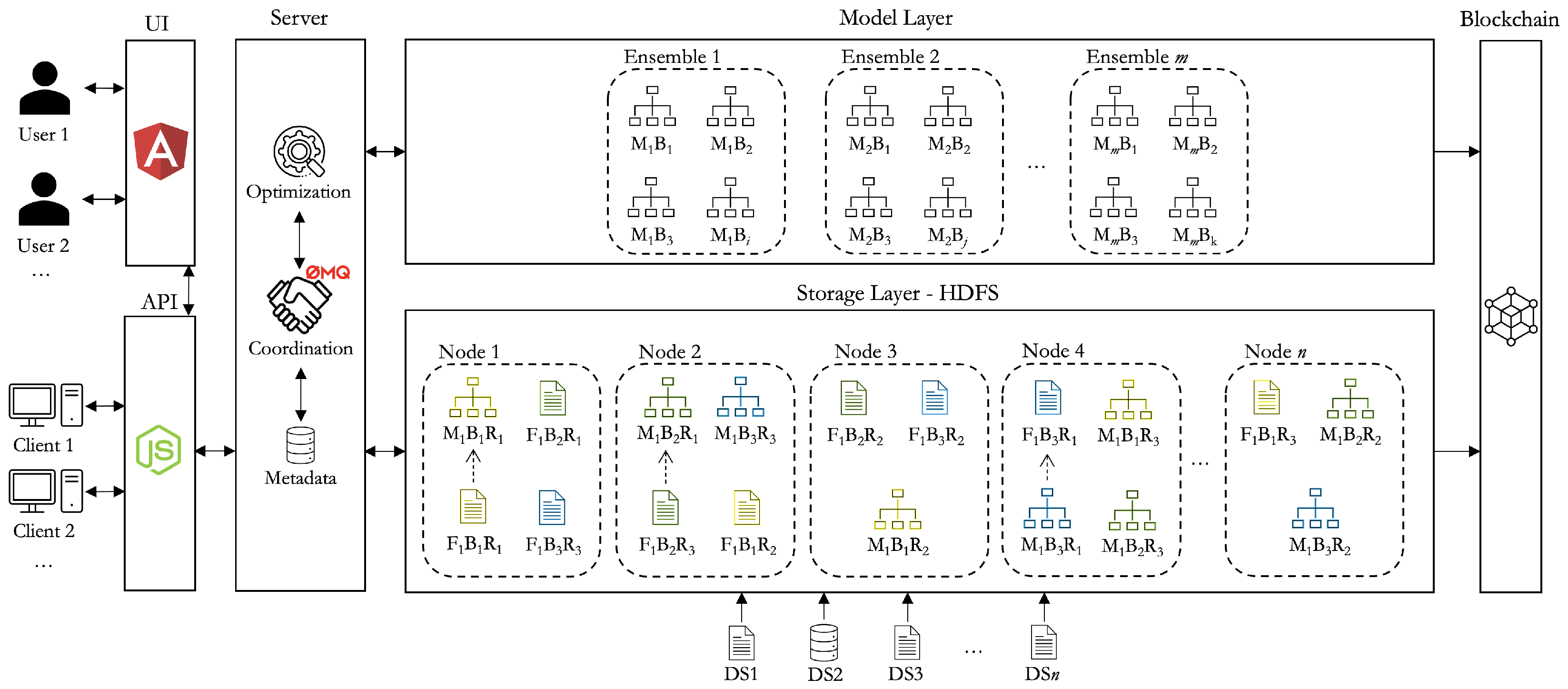
4.1. General Architecture

CEDEs is a funded research project that aims to implement dynamic and evolving distributed learning systems. One of its main goals is to maintain models up-to-date over time, with minimum computational effort. To achieve this goal, Ensemble ML models are used. These Ensembles can then be updated, over time, by including or excluding specific base models. For instance, as new data arrive, new base models are trained and may eventually replace older or worse models in the Ensemble. This is a continuous process of fine-tuning, as opposed to frequent full training of models, with the complete set of data. Moreover, the approach is highly configurable in the sense that heterogeneous Ensembles are used. That is, different types of model may constitute the Ensemble.

The whole project is based on a block-based Distributed File System (DFS) with replication. Specifically, we are using the Hadoop Distributed File System (HDFS). When a new dataset is uploaded into the HDFS, it is split into blocks. Blocks are fixed-sized parts of the original file (e.g., 128 MB) and make it possible to store a large file over a cluster of machines. Moreover, blocks are replicated according to a replication factor (e.g., 3). This means that, for any given block of a file, it will exist in n machines in the cluster, allowing clients to read from the most suitable location (according to distance or node state).

Several predetermined data processing tasks are carried out when new datasets are added. These are determined by the user and may include filtering/cleaning data, imputing data or encoding data. These tasks are implemented in the form of Spark distributed applications and run in a distributed manner across the cluster, while we manage the coordination of tasks pertaining to model training and scoring, we let the cluster manager handle these data processing tasks. The dataset is only available for training models once these user-specified operations have concluded. In some cases, such as in the case of feature encoding, some meta-data will be saved in a MongoDB distributed database. These include the encodings used since this information is necessary for later encoding the features during the prediction stage.

The secondary goal of this work is to ascertain if meta-features about each data block are relevant to predict base model training time. In the affirmative case, the extraction of these meta-features will be added to the pipeline.

4.2. Model Training

When the dataset is ready, at least one base model is trained for each block (and not for each replica). That is, when a new block is added to the HDFS, a new base model will be trained based on one of the candidate replicas. This is represented in Figure 1: the first replica of the first block of file 1 (represented by $F_1{B}_1{R}_1$), located in Node 1, is used to train a model (identified as $M_1{B}_1{R}_1$). The other two replicas of the same block, which exist in Nodes 2 and Node n are not used. This means that CEDEs implements the principle of data locality: it moves the computation to where the data is and not the other way around.

In this process, CEDEs assumes that the data may not be identically distributed, that is, there may be trends and fluctuations, and the items in different blocks (or in the same block for that matter) may be taken from different probability distributions. This may result in significant fluctuations in model performance across the base models of an Ensemble, depending on their input blocks, which is explored by the optimization module, that may use different criteria to build the best possible Ensemble (e.g., using a subset of the best models).

CEDEs also assumes that all the instances are from independent events:

$$\forall i\ne jp(x^{\left(i\right)},x^{\left(j\right)})=p\left(x^{\left(i\right)}\right)p\left(x^{\left(j\right)}\right)$$

(1)

That is, there is no relationship whatsoever between instances, including temporal/order relationships, while datasets such as these might be used in CEDEs, the algorithms implemented so far are not the most adequate for these tasks. In summary, CEDEs was designed and validated in scenarios of independent non-identically distributed data [49].

When a model is trained, it is immediately serialized and stored in the DFS. This means that it will also be replicated and that, when it is necessary for making predictions, it will simultaneously be available in multiple nodes. Moreover, multiple base models can be trained for each block, as defined by the user, while this increases the training time/cost, it also increases the likeliness of finding better models. When using CEDEs, the user may decide which algorithms to use (and their configurations) and with which proportion, or she/he may leave this to the system. If left to the CEDEs, an algorithm recommendation system is used that will suggest the best algorithm/configuration for each base model, based on the characteristics of the input data block. This recommendation system was developed in previous work and is detailed in [50].

4.3. Prediction

In CEDEs, predictions are computed following an Ensemble method. Ensembles are complex models in the sense that they are constituted by multiple so-called based models, and predictions are computed by combining the predictions of these individual base models in some way. Different approaches can be used to combine the predictions of the base models (e.g., bagging, boosting, stacking, voting). In CEDEs, predictions are computed through a weighted average, in which the weight of a model is inversely proportional to its cross-validation RMSE. The weight of a given model m in an Ensemble of n models in which ${ϵ}_i$ represents the error metric (RMSE) of model i is given by:

$$W_m=\frac{{\sum }_{i=1}^n{ϵ}_i,i\ne m}{{\sum }_{i=1}^n{ϵ}_i}\ast \frac{1}{n-1}$$

(2)

In CEDEs, the Ensemble is, however, just an abstraction: a logical construct defined by the specific base models that constitute it. That is, different Ensembles can quickly be built for each specific ML problem, by selecting from among the different available base models, according to criteria such as intended Ensemble complexity (e.g., size), cluster state, base model deprecation factor, etc.

There are thus two main tasks that must be solved by the optimization module. The first occurs when a new dataset is uploaded and the data processing pipeline finishes, and consists of selecting the nodes in which the new base models will be trained. The second occurs when a prediction is requested, and the models that will make up the Ensemble must be selected.

The work described in this paper is especially relevant for the first task. Indeed, when a new dataset is ready, a significantly large number of base models may have to be trained, easily ranging from the dozens to the hundreds. However, not only the state of the cluster will be heterogeneous (e.g., some nodes might be idle while others might be busy), but the training time of each model might also vary significantly, as our data show (Section 6 and Section 7).

Hence, having a prediction of the training time of each model is paramount for an optimal distribution of tasks across the cluster, while this distribution of tasks is currently done randomly, with the work described in this paper we will implement an optimization mechanism that takes as inputs, among other aspects, the expected training time of each base model, the candidate nodes (as the same model might be trained in different nodes, according to the replication factor), the state of the candidate nodes (some might be idle while other might have a long waiting queue), etc.

The main goal of the optimization module is thus to minimize makespan. To this end, an estimation of task duration (training time) is paramount. The rest of the paper describes how a method for predicting model training time was devised and validated.

5. Materials and Methods

As stated in Section 1, the main goal of this work is to ascertain whether it is possible to accurately predict the training time of a model, given its intended hyperparameters. Additionally, we want to determine whether characteristics about the data (meta-features) might eventually be relevant to this problem.

To answer these questions we followed an empiric data-based approach, in which an extensive number of ML experiments was carried out, and data was collected about them for analysis.

Specifically, we uploaded two datasets into CEDEs, configured with a block size of 16 MB. These two datasets, named “sales_records” and “city_temperature”, had an approximate size of 130 MB, which resulted in 8 blocks each (16 blocks in total).

For each block of each dataset, different ML models were trained. These models result from different configurations of two algorithms: Decision Trees and Neural Networks. There was no particular reason for choosing these specific algorithms. Any other algorithm would be worth analyzing, and we plan on doing so in future work.

Thus, for each algorithm, a hyperparameter grid was defined with all the intended configurations to test. Then, an exhaustive search over these hyperparameter grids was conducted, which means that a model was trained for each algorithm/configuration/block, and its performance metrics were recorded (e.g., RMSE, MAE, MSE, $r^2$). The hyperparameters were selected from among those considered, by intuition, to be more relevant for the training time. However, the particular values tested for each one were defined arbitrarily.

Table 2. Hyperparameters used for training the Decision Trees and the different values considered.

Hyperparameter	Description 1	Values
max_depth	The maximum depth of the tree	[5, 15, 25]
min_samples_split	The minimum number of samples required to split an internal node	[5, 100, 250]
max_leaf_nodes	Grow a tree with maximum n nodes, in best-first fashion. Best nodes are defined as relative reduction in impurity.	[5, 25, 50, 100, unlimited]
ccp_alpha	Complexity parameter used for Minimal Cost-Complexity Pruning. The subtree with the largest cost complexity that is smaller than ccp_alpha will be chosen.	[0.0, 0.005, 0.015]

¹ The description of the hyperparameters was obtained from https://scikit-learn.org/stable/modules/generated/sklearn.tree.DecisionTreeRegressor.html (accessed on 3 February 2023).

and

Table 3. Hyperparameters used for training the Neural Networks and the different values considered.

Hyperparameter	Description 2	Values
hidden_layers_size	The n-th element represents the number of neurons in the n-th hidden layer.	[[16,8], [16,8,4,2], [32,16,8,4,2]]
activation	The activation function used in the hidden layer.	[logistic, tanh, relu]
solver	The solver used for weight optimization.	[lbfgs, sgd, adam]
alpha	Strength of the L2 regularization term. The L2 regularization term is divided by the sample size when added to the loss.	[0.0001, 0.0005]
learning_rate	Learning rate schedule for weight updates.	[constant, adaptive, invscaling]
max_iterations	Maximum number of iterations. The solver iterates until convergence or this number of iterations. For stochastic solvers (‘sgd’, ‘adam’) this determines the number of epochs, not the number of gradient steps.	[200, 400]

² The description of the hyperparameters was obtained from https://scikit-learn.org/stable/modules/generated/sklearn.neural_network.MLPRegressor.html (accessed on 3 February 2023).

detail the hyperparameters considered for each algorithm, and their different values. In total, 2160 (3*3*5*3*16) Decision Trees and 5184 (3*3*3*2*3*2*16) Neural Networks were trained.

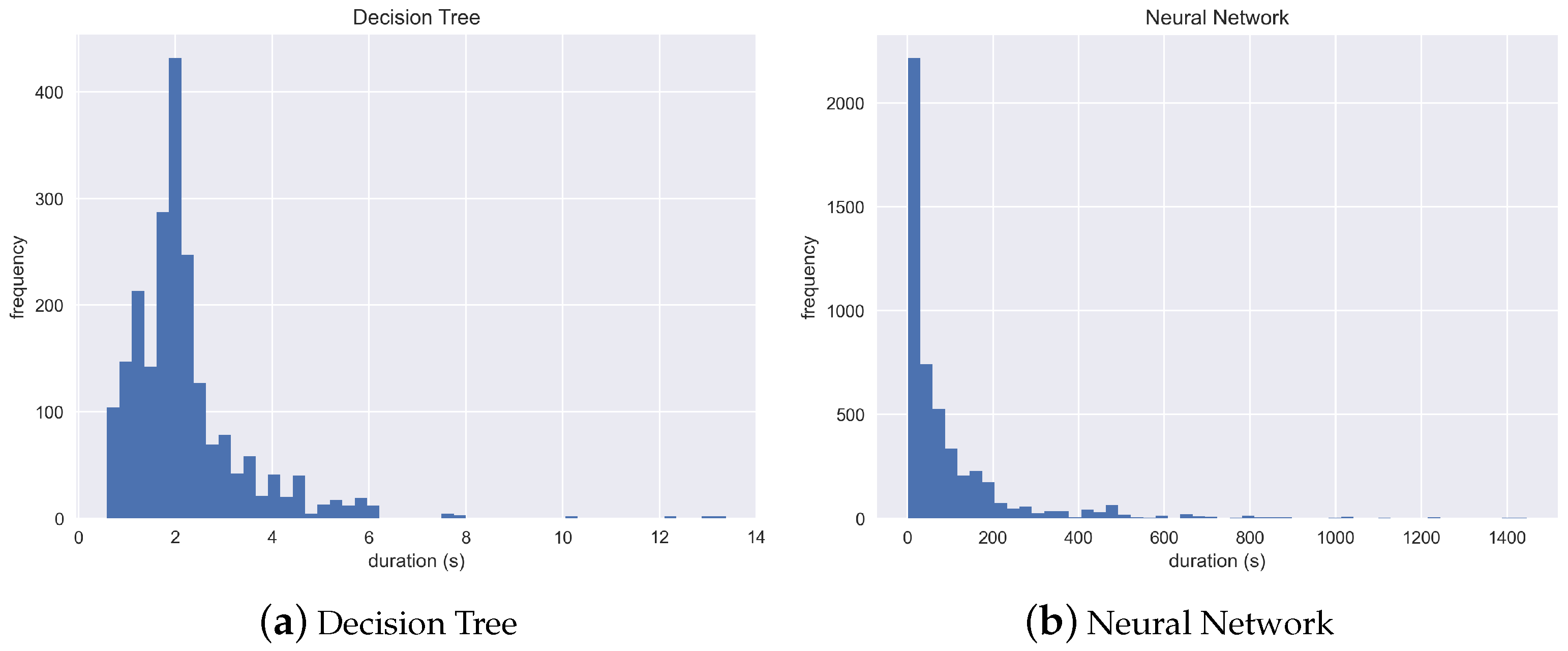
An initial analysis of these data (Figure 2) shows that the models based on the Neural Network algorithm generally take much longer to train than those based on a Decision Tree. Moreover, while the distribution of the training time is negatively skewed in both cases, the skew is more significant in the case of the Neural Networks.

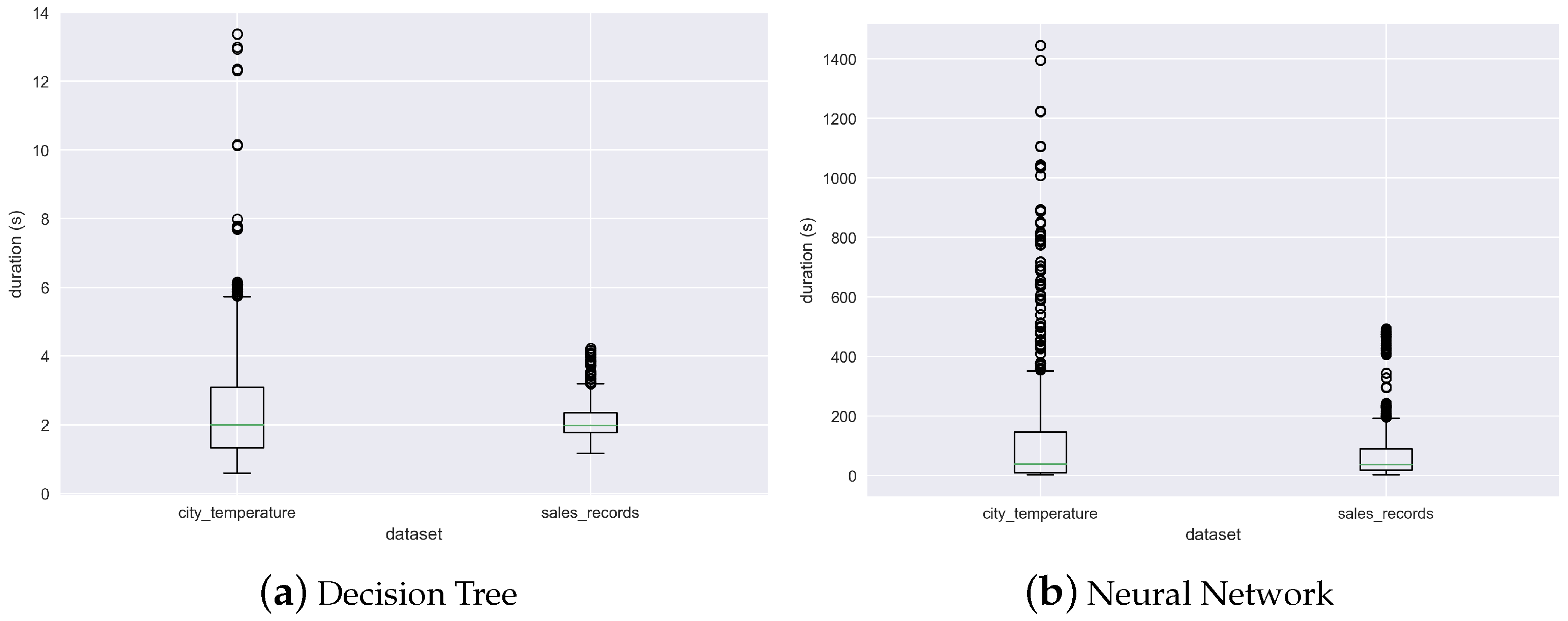
Figure 3, on the other hand, shows that the training times are quite different depending on the dataset, for both algorithms. This appears to support the second hypothesis tested in this work, that the characteristics of the data (meta-features) might have an influence on the training time of the algorithm. Potential factors for this might be different line-to-column rations, easier- or harder-to-find patterns, and different types of features (e.g., discrete vs. continuous), among many others.

Note that, as previously mentioned, in the case of this work fixed-sized blocks (16 MB are used). This means that the dataset is partitioned into different blocks, but that the number of rows in each is roughly the same. In the experiments described below, 10 input features were considered from the “sales_records”, and 6 from the “city_temperature”.

In order to assess the secondary goal of this work, which is to ascertain whether the characteristics of the data (i.e., meta-features) influence training time and can be a predictor of it, a wide range of meta-features was extracted from each block. To this end, the pymfe library (Python Meta-feature Extractor) was used [8]. This library allows for the extraction of a numerous set of meta-features for a given set of data, that essentially describe characteristics of the data (statistical and others), relations between variables, and relations with algorithm bias, among others. Several meta-feature groups are provided by this library, including general information about the dataset (e.g., number of rows or instances), statistical information, information-theoretic aspects (especially useful to describe discrete attributes and their relationship with the dependent variables), correlations between variables, complexity measures, among others. In our work, 1406 meta-features were extracted.

To summarize, 3 major groups of features were considered:

• Features that describe the characteristics of the input data (meta-features).
• Features that describe the hyperparameters of each model trained.
• Features that describe the quality/performance of each model trained (e.g., RMSE, MAE, training time), with the training time being the target variable.

These features were combined to create four different meta-datasets. The ones deemed DT and NN contain the characterisation (hyperparameters) of each Decision Tree or Neural Network trained, respectively, and the observed performance metrics for each resulting model. As previously mentioned, these datasets have, respectively, 2160 and 5184 instances. The meta-datasets deemed DT_MFE and NN_MFE contain the same data as the previously mentioned two datasets, but contain another 1406 columns with the meta-features of the input data of each model. The reason for having one meta-dataset for each algorithm is due to the fact that each model has different hyperparameters, so the meta-datasets would have different features. The alternative would be to combine the column into a single dataset, but in that case all the columns describing hyperparameters of one algorithm would be empty in the other, and vice versa, which would represent a significant amount of missing information.

With the aforementioned meta-datasets, 4 meta-models were trained, one for each meta-dataset. The process of training these meta-models was an iterative one, in which different algorithms and configurations were tested. At the end, the top model (the meta-model with the lowest RMSE) for each problem was selected to be analyzed.

Section 6 analyzes the ability of the meta-models to predict the training time of new models, while Section 7 provides a discussion of these results.

6. Results

All 4 meta-models were evaluated through 5-fold cross-validation. This means that for each of the four problems, 6 meta-models were actually trained. Five of them were trained with 80% training data and 20% test data, for the purpose of evaluating the quality of the model. Each of these meta-models was used to predict on the 20% hold-out data. The five sets of predictions were then combined and compared with the actual data, to compute the metrics described in

Table 4. Comparison of the main performance metrics for the 4 meta-models, obtained through 5-fold cross-validation on training data (metrics computed for combined holdout predictions).

Metric	DT_MFE	NN_MFE	DT	NN
MSE	0.102	1776.283	0.745	10,558.220
RMSE	0.319	42.146	0.863	102.753
$r^2$	0.935	0.925	0.527	0.555
MAE	0.103	21.263	0.536	45.625
MAE (%)	2.468%	5.618%	15.536%	18.420%

. This means that there are predictions for the whole training data, but each model making a prediction for a particular row has not seen it during training. Finally, a final version of the meta-model (the sixth one) is trained, with the full training data, and that is the main output. The cross-validation models are used only for the purpose of estimating the quality of the model.

Figure 4 details, for each meta-model, the predicted values for each real values. The solid line represents the diagonal (perfect prediction). The different folds are color-coded, to eventually identify significant error variations between folds, which could be a sign of lack of data. This has not been detected in these cases, which is a sign that the size of the datasets is enough.

With the exception of $r^2$, it must be kept in mind that the metrics provided in Table 4 are dependent on the scale of the dependent variable of the meta-model. The dependent variable is the model training time and it is measured in seconds. Given that the scales are very different for both problems, the performance of the meta-models cannot be compared directly, with the exception of $r^2$. For this purpose, we included the metric MAE (%) in the table, which was obtained through the following process.

First, to make the metric less dependent on outlier values, these were removed from the original dataset using the 1.5*IQR rule. The IQR (interquartile range) is obtained from Equation (3), in which $q_{75}$ and $q_{25}$ represent the first and third quartile, respectively.

$$iqr=q_{75}-q_{25}$$

(3)

Then, the lower and upper limits for removing outliers are given by Equations (4) and (5), respectively.

$$lower=q_{25}-1.5\ast iqr$$

(4)

$$upper=q_{75}+1.5\ast iqr$$

(5)

Next, the dataset is filtered by the variable duration, as depicted in Equation (6). In this equation, x denotes each instance of dataset X.

$$filtered=\left\{x\in X|x<upper\wedge andx>lower\right\}$$

(6)

Finally, the MAE in percentage of the scale of the dependent variable is given by Equation (7).

$$MAE(\%)=\frac{MAE}{max\left(filtered\right)-min\left(filtered\right)\ast 100}$$

(7)

The relevant values for computing the MAE in percentage, for each meta-dataset, are provided in

Table 5. Some statistics regarding the duration variable for both datasets, before and after the remotion of the outliers. These were used in the computation of the MAE(%) metric.

		#	min	max	$\overline{\mathit{x}}$	$\mathit{\sigma }$
Original	DT	2160	0.59	13.38	2.23	1.26
	NN	4980	1.63	1445.80	95.12	153.98
		$q_{25}$	$q_{75}$	IQR	lower	upper
Outlier removal	DT	1.43	2.48	1.04	−0.13	4.0
	NN	14.04	108.65	94.61	−128	250.57
		#	min	max	$\overline{x}$	$\sigma$
Without outliers	DT	1986	0.59	4.04	1.95	0.71
	NN	4536	1.63	249.27	55.82	57.98

.

From these results, it can be concluded not only that it is possible to predict model training time with a fairly good precision (main goal of this work), but also that characteristics about the data are relevant and can be used to increase the quality of the prediction (secondary goal). Given that the meta-models with meta-features perform significantly better, in Section 7 we discuss in greater depth the results, but only for these two selected models.

7. Discussion and Limitations

As seen in Section 6, the use of meta-features significantly improves the ability of the meta-model to predict the training time of a model. For this reason, the meta-models DT and NN were disregarded. This section provides some additional insights into the other two meta-models, which were trained with the inclusion of the meta-features.

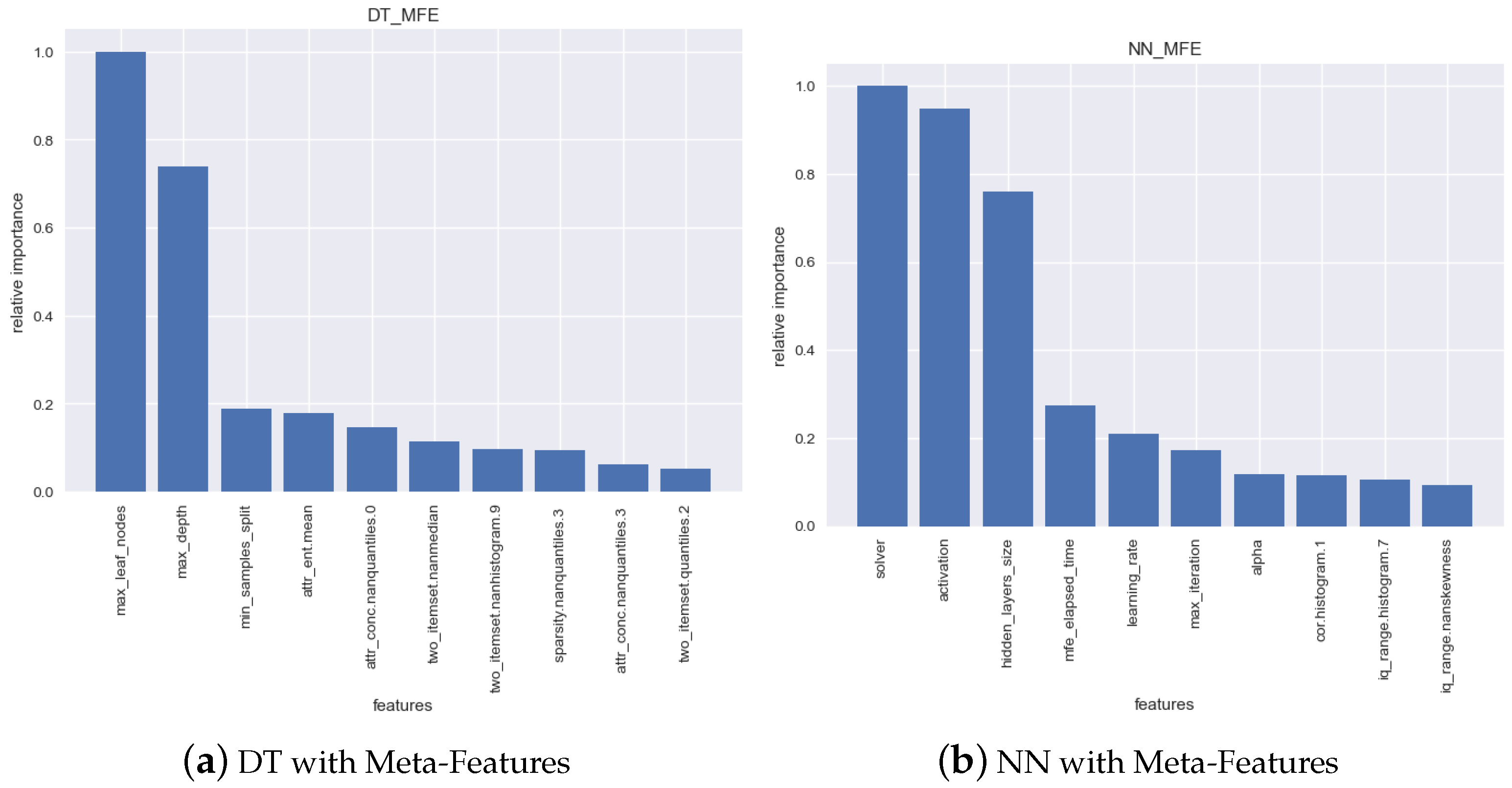
Figure 5 shows the relative importance of each feature of the meta-model, for the top-10 features. In what concerns the Decision Tree, the most relevant features are algorithm hyperparameters, notably max_leaf_nodes and max_depth. This can easily be attributed to the fact that these hyperparameters are stopping/complexity criteria, so the higher their values, the longer the model will train.

In what concerns the Neural Network, the two most relevant features are not stopping criteria: they are the solver and the activation function, which is interesting. To some extent, this shows that it will take the NN more/less time to converge depending on these hyperparameters. The third most important feature is one related to the complexity of the model: hidden_layers_size, while the latter would be expected, the significant relevance of the first two was not expected.

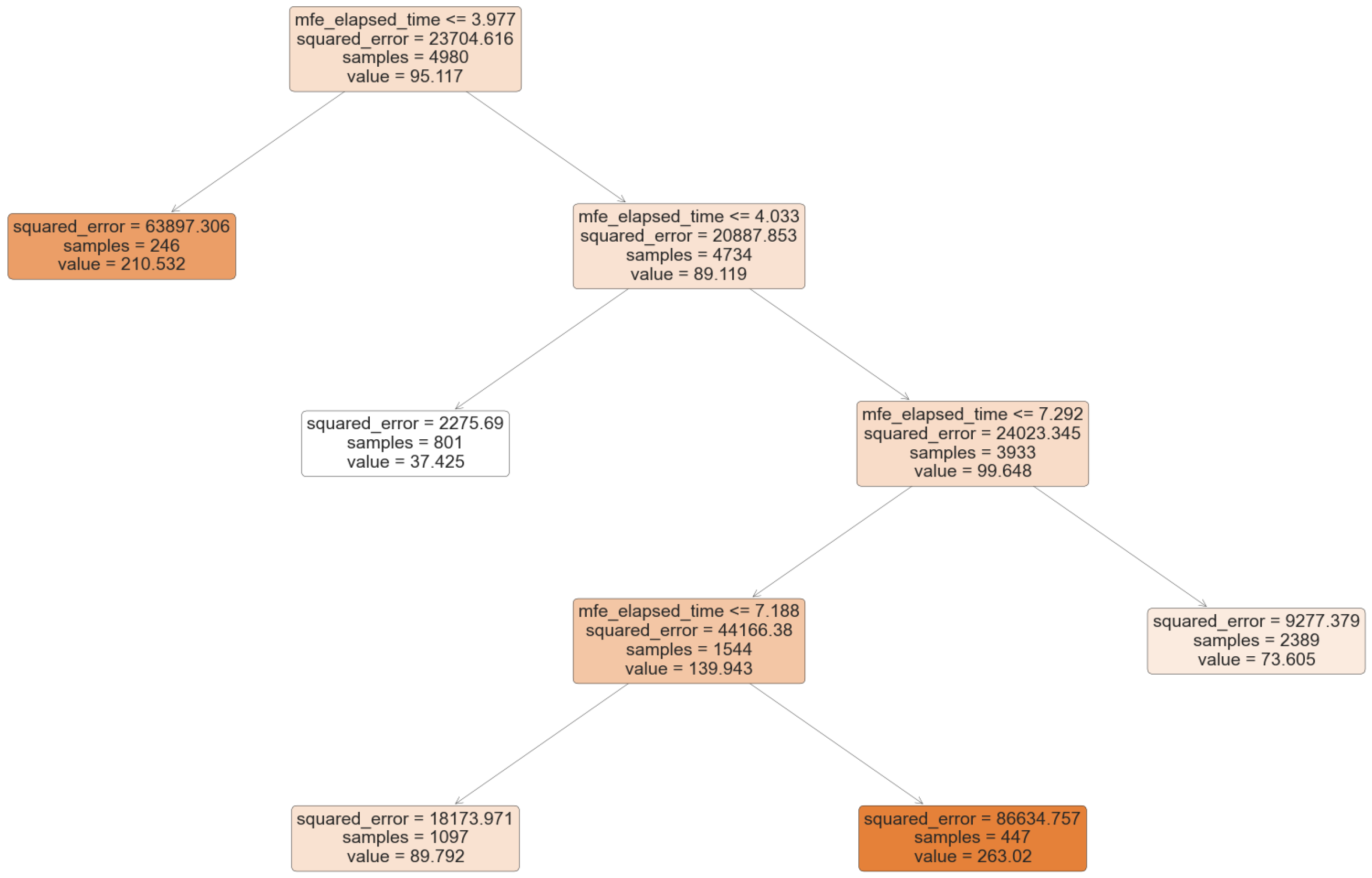
Then, another interesting insight is that, in the case of the NN, the fourth most relevant feature is the mfe_elapsed_time. This feature was created to encode the time spent in extracting the meta-features for each specific block. It could be intuited that the correlation between the training time and the meta-feature extraction time would be positive, under the assumption that both would indicate an increased complexity in the data. However, that is not the case, given that the correlation between both variables is $0.002$. This signals that, although the relationship between both features exists, it might not be linear.

To further investigate the relationship between these two features, a Decision Tree was trained (Figure 6). For the sake of interpretability, the tree was purposely oversimplified (max_leaf_nodes = 5). However, it serves the purpose of shedding some light into how the variables are related. For instance, the second highest value of training time ($210.532$) is predicted for values of mfe_elapsed_time lower than $3.977$ (although still with a significant error). The second highest training time is predicted for mfe_elapsed_time higher than $7.188$. In between, very different values can be found. This means that the relationship exists, but it is a complex one.

The following 3 relevant features for the NN are, respectively, learning_rate, max_ iteration and alpha. Given that all these features are, in one way or another, related to model complexity or stopping criteria, the relationship between them and training time is an intuitive one. The remaining three features (in the top 10) are meta-features.

To summarize, it can be concluded that the hyperparameters of the algorithms are the most relevant features when it comes to determining the training time, although characteristics of the data also play a relevant role.

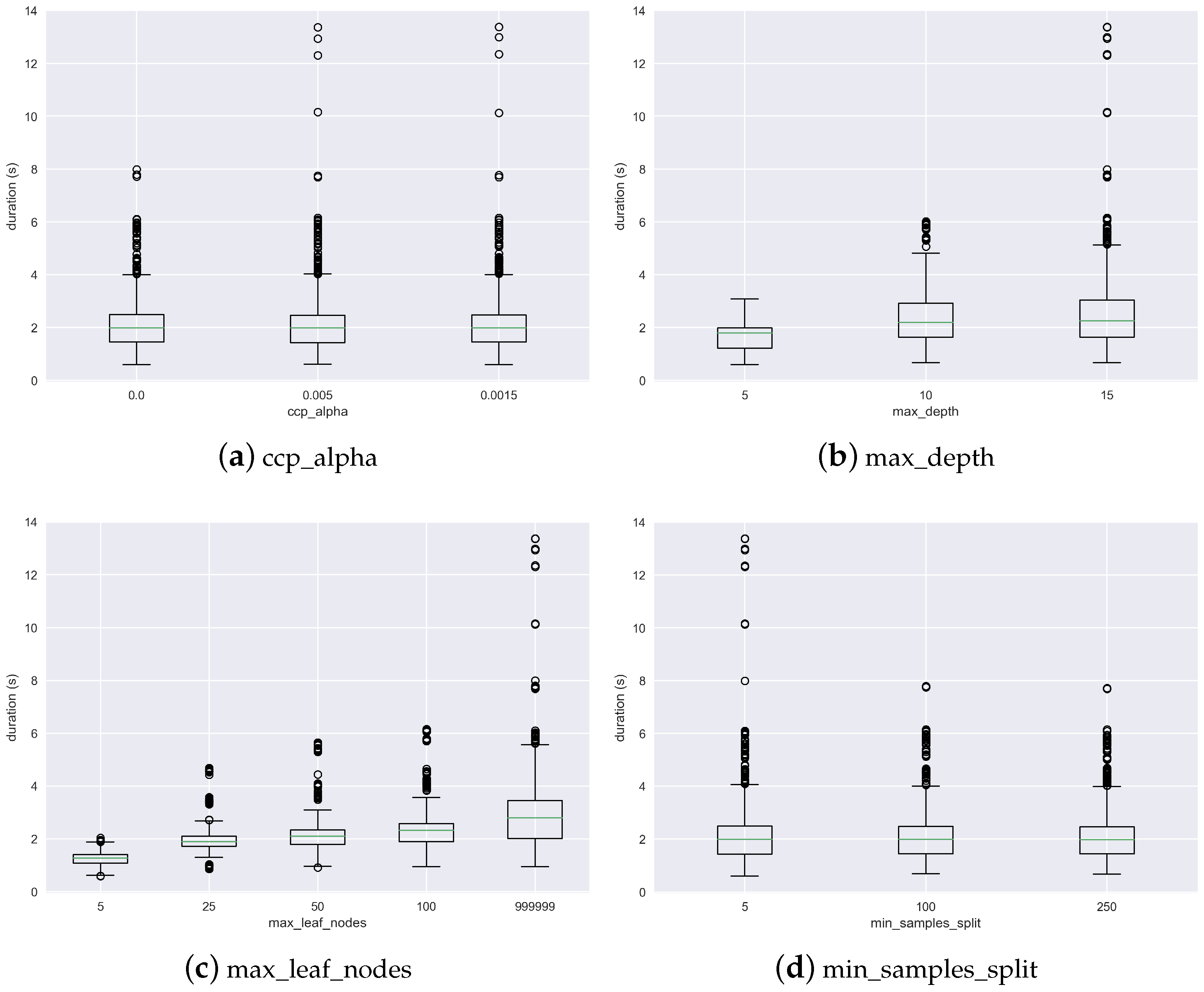
In order to better analyze the relationship between the hyperparameters and the training time, Figure 7 and Figure 8 are provided. The former shows how the 4 hyperparameters of the DTs relate to training time. It shows that training time tends to increase with a larger maximum depth of the tree, as well as with a larger number of leaves. However, it also shows that the relationship is not proportional. For instance, when the max depth is increased from 5 to 10, the training time approximately doubles. However, when it is increased to 15, it almost does not increase (save for some outliers). This might be due to the fact that, when this stopping criterion increases, the training of the tree stops for other reasons, so this hyperparameter becomes less relevant. Something similar can be observed for the maximum number of leaves.

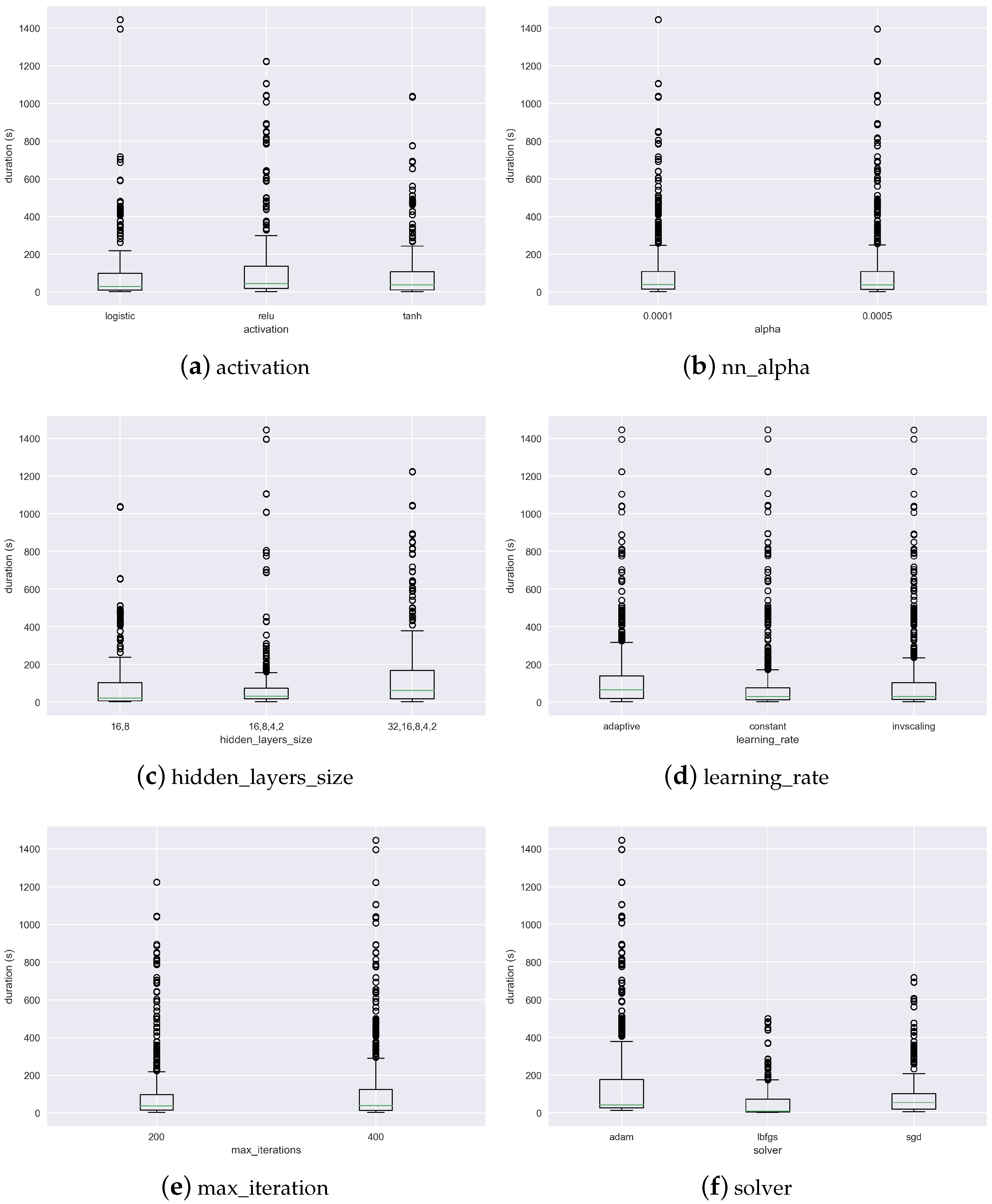
In what concerns the NN, the three hyperparameters in which the differences are visually more striking are the hidden_layers_size, the solver and the activation function. This is in line with the feature relevance plot (Figure 5). The lbfgs is the solver that is associated with a generally shorter training time. The relu activation function, on the other hand, is the one that is generally associated with longer training times.

The results presented in this section, while already interesting, must be interpreted in light of a major limitation. Given the lack of a dedicated cluster with a relevant number of computers to develop on, CEDEs was developed in the form of a Docker virtual cluster. Specifically, multiple containers based on the ubuntu:bionic image were set up, in which the Hadoop ecosystem was installed in distributed mode, including the HDFS, MapReduce and Spark frameworks. Then, on top of that, the coordination mechanisms and the two types of nodes (Coordinator and Worker) were implemented.

This means that the cluster works as it would in a real setting. However, the reported times are eventually longer than would be in a real cluster as, while distributed, all the nodes share the resources a single server. Specifically, CEDEs currently runs on an Intel^®Xeon^®Silver 4215R CPU @ 3.20 GHz with 32 GB Ram, with 8 cores (16 threads).

The provided analysis also ignores the communication overhead, which in the current setting is negligible, given that all the virtual nodes (containers) run on the same machine. However, that might not be so in a real cluster, depending on its configuration.

8. Conclusions

Distributed systems for ML are both a solution for existing challenges and a source of new challenges. In fact, once ML is seen as a distributed task, it is necessary to split data and algorithms. Moreover, it is necessary to perform task allocation in a distributed manner, across a cluster of machines, both for training models and for inference. The goal of the Continuously Evolving Distributed Ensembles (CEDEs) project is to develop a cost-effective environment for distributed training of ML models that can adapt to changes in data over time. As a result, it addresses not only the issue of learning from large datasets, but also the issue of continuously learning from streaming data in order to deal with the ongoing challenges.

CEDEs uses Ensembles in which distinct base models can be used to train blocks of data. Using block-based distributed file systems, learning tasks can be parallelized and distributed, all while adhering to the data locality principle (i.e., computation is moved to the data rather than the data being transported). The models are then combined in real time by combining them based on factors like performance and the condition of the nodes where the base models are stored. Multiple nodes can have access to the same underlying models in order to make predictions, as CEDEs store the base models in a distributed manner, which means that they are also replicated throughout the cluster.

The experiments carried out allow to conclude that it is possible to predict the training time of a model with satisfactory precision. Specifically, we are able to predict the training time of Decision Trees with an average error of 0.103 s, and the training time of Neural Networks with an average error of 21.263 s. As a basis for comparison, the training times of Decision Trees trained to build the meta-model range up to 14 s, while that of Neural Networks is over 1400 s. Given these ranges of values, the average errors for each model are considered acceptable.

The results also show that the model’s hyperparameters are generally the most relevant features in determining it. However, we also conclude that the relationship between them and the training time is neither linear nor proportional. Knowledge about these complex relationships, which are encoded in the developed meta-models, is paramount for an accurate prediction.

This work also allows to conclude that the features of the data also impact the training time of the model. This should not be counterintuitive for an experienced Data Scientist that some sets of data have simpler or more complex patterns, which obviously will influence the time to convergence of the model. In some cases, there will also be no convergence, and the model training will stop due to other time-based criteria. The size of the data is another known relevant factor. For this purpose, the effect of size was removed in this work by using a block-based distributed file system, in which all data blocks have approximately the same size (16 MB).

Another relevant contribution of this work is thus to explore this complex relationship between the characteristics of datasets and the training time of a model, and encode it in the meta-model. To the extent of our knowledge, it is the first time that this is achieved in research. In conclusion, the pipeline of data processing of CEDEs will be updated to also include the extraction of these meta-features for each block of data. These will then be used as input, together with the model’s hyperparameters, whenever a new model is trained to predict the duration of the task. The CEDEs optimization module will then use this information to decide how best to distribute tasks across the cluster, in real time.

While the work described in this paper does not address the problem of task allocation itself, it proposes what can be a valuable input for it. At this point, we expect to provide to the Optimization module a heuristic solution method to allocate and schedule the tasks considering the current cluster state and the training-time predictions obtained. An exact method could provide better results but, usually, these methods require high computational resources to obtain the optimal solution. On the other side, heuristics can provide a means to obtain good solutions (with no guarantee of achieving optimality) with considerably fewer resources as it is required to provide usability to the overall system under development.

Although the two meta-models developed were trained with data from thousands of ML experiments, in future work we will include additional datasets and algorithms, in order to have a more representative and diverse meta-dataset. Indeed, the main limitation of this work is that it only supports two algorithms so far (Decision Trees and Neural Networks). However, the main goal of the work developed so far was to validate the approach. We are confident that the performance of the approach with other metrics will be similar and that we will pursue that in future work.

We will also include additional cost variables, such as memory consumption or processor usage, so that the optimization can be performed based on multiple relevant factors, including the requirements of each model in terms of resources and the available resources in the cluster.