Investigating Trace Equivalences in Information Networks

Abstract

Equivalences are widely used and have achieved much success in concurrent systems. Meanwhile, information networks are ubiquitous for representing many complex systems and have similar characteristics and properties to concurrent systems such that they both can be described by graphs. In order to simplify information networks, we introduce equivalence to information networks, specifically leveraging the trace equivalence to reduce the complexity of these networks. In this paper, we first define the concept of trace and trace equivalence in information networks, drawing on the similar concept of concurrent systems. We then propose a computational method for determining whether two nodes are trace equivalent in an information network. With the help of this method, we derive trace-equivalent networks from original networks. Experiments show that we are able to reduce the number of nodes in the ACM and DBLP datasets by at most 65.21% and 46.68%, respectively. Running the PathSim algorithm on the original and derived networks, the mean error is 0.0728 in ACM and 0.0446 in DBLP. Overall, the results indicate that the derived networks have fewer nodes and edges than the original networks, yet still capture the same or similar information. By using trace equivalence, we are able to simplify information networks and improve their efficiency while preserving most of their informational content.

1. Introduction

In concurrent systems, a process is the behavior of a system, and the study of process is referred to as process theory [1,2]. Process theory is concerned with two main activities: modeling and verification. Modeling is about representing processes, and verification is about proving statements of processes. Labeled transition systems and process graphs are commonly used to represent processes. To prove that the actual behavior of a system matches its intended behavior, semantics are used as a criterion to determine whether two processes are equal. Furthermore, the linear time-branching time spectrum [3] illustrates various semantics that can be used to simplify systems. This spectrum is formed by semantics that is partially ordered by the relation “makes strictly more identifications on processes than” [1,3,4]. Based on certain semantics, equivalence indicates that two processes behave similarly and can be used to simplify systems by reducing duplicate or similar branches of behaviors in concurrent systems [5], while still preserving information of the system.

Trace semantics [6,7,8] is the coarsest in the linear time-branching time spectrum, meaning that it makes the most identifications of any of the other semantics. In trace semantics, the behavior of a system is represented as a sequence of actions, called a trace, that is generated by the system as it executes. According to trace semantics, two processes are considered equivalent if they allow the same set of traces. Trace equivalence is based on trace semantics and can capture identical or similar behaviors, allowing concurrent systems to be simplified by removing redundant or unnecessary branches. Trace equivalences have been applied in a variety of fields, such as linear algebraic hybrid systems [5], security properties of cryptographic protocols [9], and polynomial algebraic event structure [10,11].

Information networks have gained a lot of attention from researchers in recent years for their ability to model real-world systems. These networks can represent a wide range of scenarios, from molecules and social networks to bibliography networks, e-commerce, and advertising. Due to powerful representation ability, various tasks have achieved good performance results, including node classification, link prediction, and recommendation [12,13,14,15,16]. Most of the state-of-the-art research has employed graph neural network techniques [17,18,19,20,21,22,23,24]. Graph neural networks are a class of neural networks that are designed to process data with a graph structure and use a message-passing mechanism to continuously aggregate the information from nodes and their neighborhoods. Through this approach, each node contains a summary of information from its neighboring nodes. The adjacency matrix and the features of each node are then fed into the graph neural network for training to obtain the final embedding of each node. With the final embedding of each node, we can do downstream tasks, such as classifications, predictions, and recommendations.

As modern society becomes more complex, information networks are becoming increasingly complicated due to the vast amount of information they contain. This results in these networks having a larger number of identical or similar pieces of information. For example, in an e-commerce scenario, different users are more likely to buy or click on the best-selling products on the website, leading to similar or even identical purchase information. Graph neural networks do not explicitly distinguish nodes with identical or similar information, and this can cause problems with information duplication. When nodes with similar information are aggregated and processed, it can lead to information redundancy in the final results, which can harm the accuracy of downstream tasks. To address this issue, it is important to consider similar information between nodes when performing information aggregation and graph neural network training. Additionally, as information networks become more complex, the number of nodes and edges in these networks is also increasing. This reminds us of the “state explosion” problem in concurrent systems, where the large number of possible states can make it difficult to analyze and verify the behavior of the system. Trace equivalence in concurrent systems can alleviate the “state explosion” problem by removing duplicate branches of processes. The relationships among entities in information networks indicate the transmission of information in these networks, which can be thought of as traces in concurrent systems. Based on this intuition, trace equivalence can be applied to remove duplicate information in information networks that consist of relationships. This can help to simplify information networks and improve the accuracy of downstream tasks.

In this paper, we propose the use of trace equivalence to simplify information networks. To do this, we first need to clarify which objects of information networks can be reduced through equivalence. In concurrent systems, these objects are known as “states” and “transitions”. With these objects in mind, we define the concepts of trace and trace equivalence in information networks. We also provide a method for determining when two nodes are trace equivalent. By applying trace equivalence to the nodes of information networks, we can obtain trace-equivalent networks that are simplified versions of the original information networks. Finally, to verify that the trace-equivalent network maintains the information of the original network, we perform the same data mining tasks on both networks and compare the results to ensure that the output of the data mining algorithms is consistent or similar.

The main contributions of this paper are as follows:

• We provide a characterization of trace semantics and trace equivalence in information networks, and we give a computational method for computing trace equivalence in information networks.
• We conduct trace equivalence computational tasks on information networks to obtain trace-equivalent networks from the original networks, and show that these derived networks have a smaller number of nodes and edges.
• We show that conventional data mining algorithms can achieve the same or similar results on both the original networks and their trace-equivalent networks.

2. Materials and Methods

2.1. Review of Information Networks

In this section, we recall some concepts and notations used throughout the paper.

An information network [14] can be modeled as a graph $G=(V,E,O,R)$, in which V is the set of entities(nodes), E is the set of relations(edges) among these entities. $\left|O\right|=m$ represents the number of entities, $\left|E\right|=n$ represents the number of relations, and O and R are the set of node types and edge types, respectively. Mapping function $\phi :V\to O$ maps each node $v\in V$ to a node type $o\in O$ and mapping function $\psi :E\to R$ maps each edge $e\in E$ to an edge type. In the situation that $\left|O\right|+\left|R\right|>2$, the information network is named heterogeneous information networks. Otherwise, it is homogeneous information network.

Adjacency matrix [14] is represented as $A\subseteq {\mathbb{R}}^{n\times n}$, n is the number of nodes in information networks. $A_{i,j}=1$ indicates that there is an edge between node i and node j. Otherwise, $A_{i,j}=0$ indicates no edge.

It is shown in Figure 1 that a small information network abstracts from the DBLP information network. There are seven entities in this network, including three authors, two papers, and two venues. The set of entities of this network is formally denoted as $V=\{a_1,a_2,a_3,p_1,p_2,v_1,v_2\}$. And the set of relations is $E=\{a_1\stackrel{write}{\to }{p}_1,a_2\stackrel{write}{\to }{p}_1,a_2\stackrel{write}{\to }{p}_2,a_3\stackrel{write}{\to }{p}_1,a_3\stackrel{write}{\to }{p}_2,p_1\stackrel{publish}{\to }{v}_1,p_2\stackrel{publsh}{\to }{v}_2\}$. The set of entity types O and relation types R is $\{author,paper,venue\}$ and $\{write,publish\}$, respectively. Furthermore, the adjacency matrix of this network is illustrated in Figure 2 in which each row and each column represents an entity, and each element of this matrix represents the relation of the corresponding pair of entities. The notations used in this paper are illustrated in

Table 1. Notations.

Notation	Explanations
G	an Information Network
V	set of nodes
E	set of edges
O	set of node types
R	set of edge types
A	adjacency matrix
$v,v_i$	node
$e,e_i$	edge
$P\left(v_i\right)$	path set of node $v_i$
$T\left(v_i\right)$	trace set of node $v_i$
${=}_T$	trace equivalence

.

2.2. Methods

In this section, we theoretically introduce the idea of trace equivalence to information networks. We first give the concept of “states” and “actions” in information networks. Employing these concepts, we come up with the trace semantics of information networks inspired by the trace semantics of process theory in concurrent systems. Further, we show the computational method to determine whether two nodes are trace equivalent in information networks for deriving trace-equivalent networks from original networks. Moreover, to verify the maintainability of information in trace-equivalent networks, we conduct experiments on both the original networks and their trace-equivalent networks.

2.2.1. Trace Semantics of Information Networks

In the process graph, states and transitions are the node and edges. Equivalences are then used to reduce the duplicate branches by removing equivalent states. Inspired by this, we leverage equivalence by treating nodes in information networks as states and edges as transitions in information networks. Nevertheless, we still use nodes and edges in the subsequent sections for the generality of research.

To begin, we come up with the concept of the trace in information networks according to the concepts in concurrent systems [4]. Information networks are usually represented as graphs, where nodes are entities and edges are relations between entities. Regarding nodes in information networks as states in process theory, the concept of trace in information networks is defined as follows according to the trace semantics of process theory.

Definition 1.

Trace in information networks.Given an information network $G=(V,E,O,R)$, a path starting from node $v\in V$ is represented as $p:v\stackrel{e_1}{⟶}{v}_1\cdots \stackrel{e_n}{⟶}{v}_n$, where $v_i\in V$ and $e_i\in E$. A trace of this path is formally denoted as $e_1{e}_2\cdots e_n$ based on the path. The set of paths starting from node v is denoted as $P\left(v\right)$, and the set of traces is denoted as $T\left(v\right)$, respectively.

Note that a path is in the form of a node followed by an edge repeatedly, while continual edges composite a trace. Consequently, a trace describes and focuses on the relationship between two nodes since a trace is the edge sequence of a path starting from one node to another node, i.e., in a social network, if two people follow the same one, their relationship is common-follow, or if they follow each other, their relationship is mutual-follow.

Trace semantics of process is based on the idea that two processes are identified if they allow the same set of sequences of actions. In information networks, similarly, trace semantics are described as two nodes to be identified if they have the same set of relationships with other nodes. Moreover, it is significant that two nodes be identified if and only if they are of the same type. With Definition 1, we define trace equivalence as follows.

Definition 2.

Trace equivalence in information networks.Given an information network $G=(V,E,O,R)$, two nodes v, w aretrace equivalentif and only if they are of the same type and their sets of traces are equal. Trace equivalence is formally represented as $T\left(v\right)=T\left(w\right)\wedge \phi \left(v\right)=\phi \left(w\right)$ and, for simplicity, notated as $T\left(v\right)=T\left(w\right)$ or $v{=}_{T}w$.

For example, in Figure 1, we show that in a small example abstracting from the DBLP bibliography network, in which there are three authors $a_1$, $a_2$ and $a_3$, two papers $p_1$, $p_2$, and two venues $v_1$, $v_2$, the path set of $a_1$ is

$$\begin{array}{c}\hfill P\left(a_1\right)=\{a_1\stackrel{write}{\to }{p}_1,a_1\stackrel{write}{\to }{p}_1\stackrel{publish}{\to }{v}_1\},\end{array}$$

then the trace of author $a_1$ is

$$\begin{array}{c}\hfill T\left(a_1\right)=\{write\left(p_1\right),write\left(p_1\right)\circ publish\left(v_1\right)\},\end{array}$$

similarly, the path set of $a_2$ is

$$\begin{array}{c}\hfill P\left(a_2\right)=\{a_2\stackrel{witer}{\to }{p}_1,a_2\stackrel{write}{\to }{p}_1\stackrel{publish}{\to }{v}_1,a_2\stackrel{write}{\to }{p}_2,a_2\stackrel{write}{\to }{p}_2\stackrel{publish}{\to }{v}_2\},\end{array}$$

and the path of $a_3$ is

$$\begin{array}{c}\hfill P\left(a_3\right)=\{a_3\stackrel{write}{\to }{p}_1,a_3\stackrel{write}{\to }{p}_1\stackrel{publish}{\to }{v}_1,a_3\stackrel{write}{\to }{p}_2,a_3\stackrel{write}{\to }{p}_2\stackrel{publish}{\to }{v}_2\},\end{array}$$

and it is significant that authors $a_2$ and $a_3$ are trace equivalent since they are of the same type of $author$ and their sets of traces both are

$$\begin{array}{c}\hfill T\left(a_2\right)=T\left(a_3\right)=\{write\left(p1\right),write\left(p2\right),write\left(p_1\right)\circ publish\left(v_1\right),write\left(p_2\right)\circ publish\left(v_2\right)\}.\end{array}$$

Moreover, $T\left(a_1\right)\subset T\left(a_2\right)$ reveals that the interactions of author $a_2$ with other nodes contain the interactions of author $a_1$. We stipulate this situation as approximate trace equivalent because their sets of traces have common items but are not totally equal.

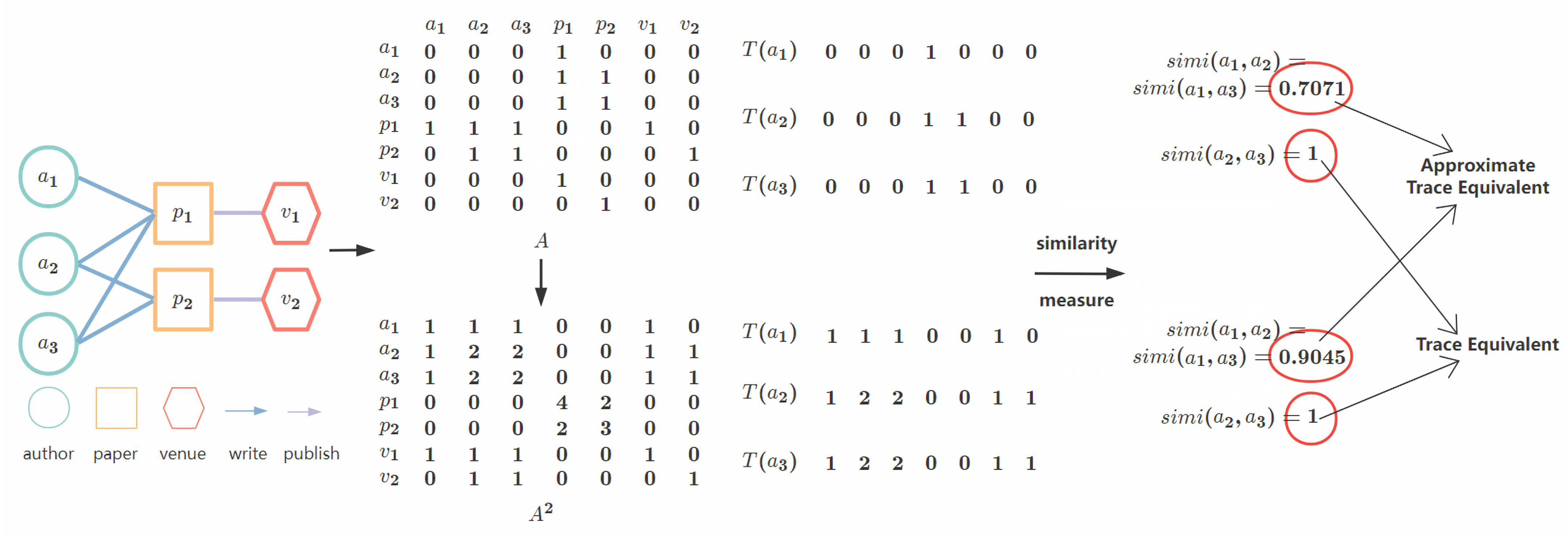
2.2.2. Computational Method of Trace Equivalences

Continuing with the concept of trace equivalence between nodes, we further give the computational method of trace equivalences in a mathematical way. In this regard, we need to represent an information network in mathematical form so that we leverage the adjacency matrix of an information network to reflect the messages we need mathematically. Given an information network $G=(V,E,O,R)$, an adjacency matrix of G is represented as $A\in {\mathbb{R}}^{n\times n}$. $A_{i,j}=1$ if there is an edge between node i and node j such that these two nodes are connected and related; otherwise, $A_{i,j}=0$ means node i and node j have no edges, yet they are not related. $A_i$ can be used to depict all the paths whose start node is node i. Adjacency matrix A illustrates the relationships of every node with other nodes in the network, and with the adjacency matrix, we can describe the path information and further the trace information of every node.

A primitive adjacency matrix A not only describes the relationship of each node but also reflects all the paths in the network, where the length of all these paths is equal to 1. Moreover, the trace sets of these paths can also be described by the adjacency matrix A. $A_{i,j}$ means that there is a trace of node i indicating its relationships with node j. Furthermore, the matrix A multiplied by itself can be seen as a concatenation of two 1-length paths, where the end node of the former path is the same as the first node of the latter path. In this way, we can obtain the 2-length paths of the network. Repeating this procedure n times, we can acquire the n-length paths of the network. Formally, we use $A^n$ to represent all the n-length paths of the network and yet traces.

Cosine Similarity [25] Cosine similarity is a measure of similarity between two non-zero vectors of an inner product space that measures the cosine of the angle between them. In other words, it determines the orientation of the vectors rather than their magnitude. The smaller the angle between the vectors, the higher the cosine similarity. Formally, given two vectors A and B, the cosine similarity score of A and B can be calculated by

$$similarity(A,B)=\frac{A·B}{\left|A\right|\left|B\right|}=\frac{{\displaystyle \sum _{i=1}^n}{A}_i{B}_i}{\sqrt{{\displaystyle \sum _{i=1}^n}{A}_i^2}\sqrt{{\displaystyle \sum _{i=1}^n}{B}_i^2}}$$

(1)

According to this equation, cosine similarity requires normalizing firstly the length of the two vectors A, B, then measuring the direction of the two vectors and finally resulting in a score of similarity of the two vectors. Cosine similarity is widely used in many research fields, such as natural language processing, information retrieval, and recommendation systems [25,26]. It has the advantageous feature that it is equal to 1 for identical vectors and 0 for orthogonal vectors when all elements of the vector are greater than 0.

In this paper, with adjacency matrix A of an information network indicating the traces deriving from 1-length paths of this network, we use A to show how to calculate the cosine similarity of traces. For two nodes i and j of an information network, their similarity score can be directly calculated by performing cosine similarity of the two vectors $A_i$ and $A_j$, then the similarity score of these two nodes is calculated by the equation $similarity(A_i,A_j)=\frac{A_i·A_j}{|A_i\left|\right|A_j|}$.

With the similarity score of traces of two nodes, we can say that two nodes are trace equivalent if and only if $similarity(A_i,A_j)=1$. Furthermore, since these vectors are used to represent sets of traces, elements of these vectors are usually greater than or equal to 0. The similarity score of each node pair is thus greater than or equal to 0. Based on this property, we stipulate that two nodes i and j are approximate trace equivalent if and only if $0<similarity(A_i,A_j)<1$.

Alongside the example in Figure 1, we show the computation steps in Figure 2. Considering three authors in this figure, the adjacency matrix A shows the relations held by three authors and describes the 1-length path of three authors and the traces corresponding to these paths. For the longest meaningful path with a length equal to two in this example, we iterate the matrix multiplication one time to obtain $A^2$ and obtain the 2-length paths of the information network. We then obtain the vectors representing the traces of every node from these paths. The trace sets of three authors are represented by vectors as follows.

For author $a_1$, the trace sets are

$$\begin{array}{c}\hfill \left[\begin{array}{ccccccc}0& 0& 0& 1& 0& 0& 0\end{array}\right],\\ \hfill \left[\begin{array}{ccccccc}1& 1& 1& 0& 0& 1& 0\end{array}\right],\end{array}$$

for author $a_2$, the trace sets are

$$\begin{array}{c}\hfill \left[\begin{array}{ccccccc}0& 0& 0& 1& 1& 0& 0\end{array}\right],\\ \hfill \left[\begin{array}{ccccccc}1& 2& 2& 0& 0& 1& 1\end{array}\right],\end{array}$$

and for author $a_3$, the trace sets are

$$\begin{array}{c}\hfill \left[\begin{array}{ccccccc}0& 0& 0& 1& 1& 0& 0\end{array}\right],\\ \hfill \left[\begin{array}{ccccccc}1& 2& 2& 0& 0& 1& 1\end{array}\right],\end{array}$$

Applying the cosine similarity measure on each pair of three authors, we obtain the similarity score of each pair:

$$\begin{array}{c}\hfill similarity(a_1,a_2)<1,\\ \hfill similarity(a_1,a_3)<1,\\ \hfill similarity(a_2,a_3)=1.\end{array}$$

The results exhibit that authors $a_2$ and $a_3$ are trace equivalent since their similarity score is 1, $a_1$ and $a_2$ are approximate trace equivalent since their scores are less than 1, and $a_1$ and $a_3$ are approximate trace equivalent as well.

For more complex networks, we will iterate the matrix multiplication of adjacency matrix more than two times to fetch more traces and provide more details when determining whether two nodes are trace equivalent. For an information network, we will iterate n times to get $\{A,A^2,\cdots ,A^n\}$, which also describes the traces of this information network, and based on traces of every node, we can calculate the similarity score by applying the similarity score function (cosine similarity in this paper).

2.2.3. Derive Trace-Equivalent Networks

With the computational method of trace equivalence, we determine whether two nodes are trace equivalent by computing the similarity score between them in an information network. This section will investigate how to derive a trace-equivalent network from a given information network. Given an information network $G=(V,E,O,R)$, after performing the similarity measure of an information network, we acquire many tuples of trace equivalent nodes in a mathematical way such that $(i,j)$ where i and j are the nodes of information network G, and $T\left(i\right)=T\left(j\right)$. We use $TE\left(G\right)$ to denote the set of all the tuples of trace-equivalent nodes of information network G, formally as

$$\begin{array}{c}\hfill TE\left(G\right)=\left\{\right(i,j\left)\right|T\left(i\right)=T\left(j\right),i\in V,j\in V\}\end{array}$$

where $TE\left(G\right)$ encapsulates the rough trace equivalent node tuples of an information network. In $TE\left(G\right)$ of an information network G, the same node can appear in different tuples. The nodes in these different tuples are trace equivalent by the transitive of trace equivalence. We group these nodes by trace equivalence and merge all nodes in these tuples into the same set, which is named the trace-equivalence class.

We use $TEClass$ to formally represent these trace-equivalence classes of the information network G. Each element of $TEClass$ is a group of nodes that are trace equivalent to one another, meaning they have the same trace in the network. The $TEClass$ can be formally noted as

$$\begin{array}{c}\hfill TEClass=\left\{N\right|\forall i,j\in N,T\left(i\right)=T\left(j\right),N\subset V\}\end{array}$$

With the concept of trace-equivalence classes $TEClass$, we are able to simplify the representation of the information network G. By reducing nodes based on these trace-equivalence classes, we can derive a trace-equivalent network. To accomplish this, we select a representative node from each set in $TEClass$, which will be used to replace all nodes in that particular set. The generated trace-equivalent network not only simplifies the original network, but also maintains the essential information. It is a smaller and more manageable network, while still accurately reflecting the trace relationships between nodes. With this basis, we optimize the $TEClass$ as

$$\begin{array}{c}\hfill TEClass=\{i\to N|i\in N,\forall j\in N,T\left(i\right)=T\left(j\right),N\subset V\},\end{array}$$

where i is the representative node of a trace-equivalence class N. The optimized formula can be easily used in the process of node reduction by using i to replace N.

In Figure 3, continuing with the example in Figure 2, we demonstrate the procedure of generating equivalence classes and choose one representative node of each equivalence class on behalf of the whole class. Subsequently, we can derive the trace-equivalent network from the original information network. In this simple example, $TE\left(G\right)=(a_2,a_3)$ only contains one tuple, and hence, it is also the only equivalence class of this network. We choose $a_2$ to represent the whole equivalence class, and the result shows that one node and two edges are reduced in the new trace-equivalent network.

We use $G_{TE}=GmodTE\left(G\right)$ to formally represent the derived network in which notation $mod$ represents the procedure of reducing nodes by trace equivalences. $G_{TE}$ encapsulates the complete structural information of the original network, which describes the relationships of the network, representing each equivalence class with one specific node, making it possible to reduce duplicate nodes and edges of the information network while preserving structural information. The representative nodes and edges of the same equivalence class hold the information of reduced nodes and edges. To state the method of deriving trace-equivalent networks more clearly, we summarize the above steps into Algorithm 1.

Algorithm 1: Deriving trace-equivalent network from an given network.

With the $G_{TE}$ having fewer nodes and edges than the original, it is possible to accelerate data mining algorithms since less information leads to fewer computations while executing these algorithms. Another problem we need to figure out is, though less information leads to fewer computations, the accuracy of these algorithms while maintaining consistent or approximate accuracy of the original network. In this paper, we choose the Pathsim algorithm to verify the maintainability of data mining algorithms on both G and $G_{TE}$. We prove that the accuracy of Pathsim algorithms on G and $G_{TE}$ is consistent.

Definition 3.

Pathsim[27]. Given an information network G, Pathsim measures the correlation of two entities x and y under a meta-path $\mathcal{P}$. The core component of the Pathsim algorithm is as follows.

$$s(x,y)=\frac{2\times \left|\right\{p_{x⇝y}:p_{x⇝y}\in \mathcal{P}\left\}\right|}{|\{p_{x⇝x}:p_{x⇝x}\in \mathcal{P}\}|+|\{p_{y⇝y}:p_{y⇝y}\in \mathcal{P}\}|}$$

(2)

where $p_{x⇝y}$ is a path instance between x and y, $p_{x⇝x}$ is a path instance between x and x and $p_{y⇝y}$ is a path instance between y and y. For elaboration, a meta path $\mathcal{P}$ is defined on $(O,R)$ and denoted as $O_1\stackrel{R_1}{\to }{O}_2\stackrel{R_2}{\to }\cdots \stackrel{R_l}{\to }{O}_{l+1}$ so that it illustrates the relation between node types.

Theorem 1.

The results of Pathsim are consistent on the original network G and its trace-equivalent network $G_{TE}$, i.e., the results of Pathsim are maintainable.

Proof. 

Given an information network $G=(V,E,O,R)$, node $v_1\in V$ and node $v_2\in V$ are trace equivalent. Then, for every reachable node $v_r\in V$ from node $v_1$ and $v_2$, $v_r\ne v_1\ne v_2$,

$Pathsim(v_1,v_r)=\frac{2\times \left|\right\{p_{v_1⇝v_r}\left\}\right|}{|\left\{p_{v_1⇝v_1}\right\}|+|\left\{p_{v_r⇝v_r}\right\}|}$,

$Pathsim(v_2,v_r)=\frac{2\times \left|\right\{p_{v_2⇝v_r}\left\}\right|}{|\left\{p_{v_2⇝v_2}\right\}|+|\left\{p_{v_r⇝v_r}\right\}|}$,

Because node $v_1$ and node $v_2$ are trace equivalent,

$T\left(v_1\right)=T\left(v_2\right)$,

then for node $v_r$, the trace from node $v_1$ to node $v_r$ and the trace from node $v_2$ to node $v_r$ are equal.

Based on Definition 1, the paths from node $v_1$ to node $v_r$ and the paths from node $v_2$ to node $v_r$ are identical.

Then, $|\left\{p_{v_1⇝v_r}\right\}|=|\left\{p_{v_2⇝v_r}\right\}|$.

Similarly, we can obtain $|\left\{p_{v_1⇝v_1}\right\}=|\left\{p_{v_2⇝v_2}\right\}$,

So, $Pathsim(v_1,v_r)=Pathsim(v_2,v_r)$.

In $G^{\prime }s$ trace-equivalent network $G_{TE}$, $v_1$ and $v_2$ are in the same equivalence class. We choose $v_1$ to represent this equivalence class. With $Pathsim(v_1,v_r)=Pathsim(v_2,v_r)$, the results of Pathsim are consistent.

Therefore, the results of Pathsim are maintainable. □

Trace equivalence indicates that $similarity(v_1,v_2)=1$. Meanwhile, approximate trace equivalence indicates $similarity(v_1,v_2)<1$. The smaller the $similarity(v_1,v_2)$, the greater the difference of the Pathsim results between them. In the next section, we verify that our proof is correct through experiments.

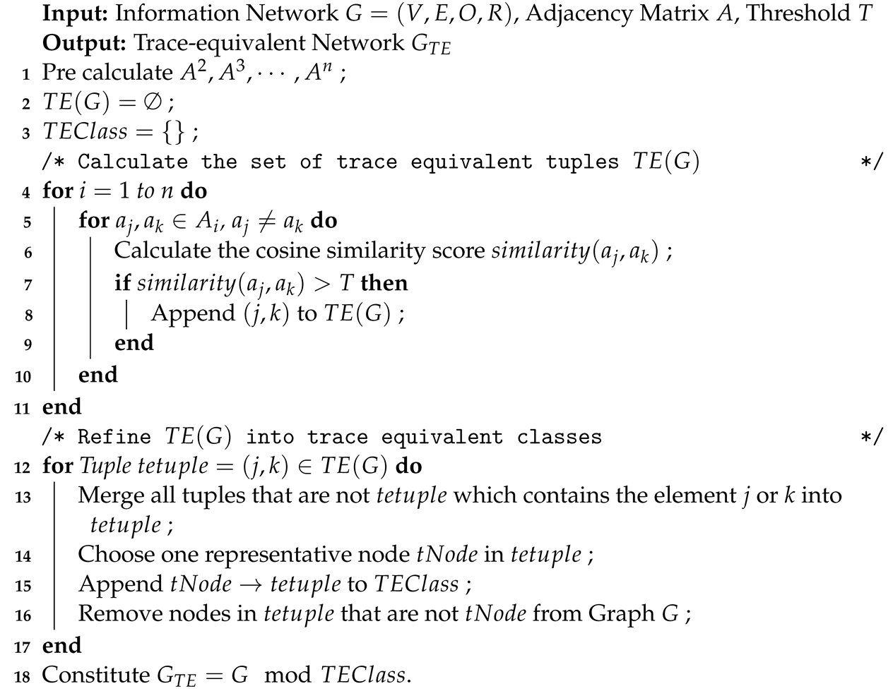
3. Experiments and Discussion

In this section, we experiment on public real-world datasets to verify the availability of reduction by trace equivalence in information networks and verify the maintainability of data mining algorithms between trace-equivalent networks and original networks.

3.1. Datasets

We use the public ACM and DBLP datasets in [28]. ACM and DBLP datasets are both bibliographic networks of academic publications. These two datasets are representative information networks and are widely used in various tasks.

ACM. The ACM dataset from [28], also known as HGBn-ACM, is utilized in this study. It consists of four types of entities: 5959 authors (A), 3025 papers (P), 1902 terms (T), and 56 subjects (S). The relationships in the dataset are established through connections, such as 9949 paper–author (P-A), 5343 paper–paper (P-P), 3025 paper–subject (P-S), and 225,619 paper–term (P-T) connections. This paper focuses on the author (A) type due to the availability of labeled nodes, allowing for a further investigation into their label consistency under trace equivalence. Our task is to reduce the number of author nodes in the dataset through trace equivalence.

DBLP. The DBLP dataset, originating from [28], is known as HGNn-DBLP. It consists of four types of entities: 4057 authors (A), 14,328 papers (P), 7723 terms (T), and 56 venues (V). The relationships in the dataset are established through connections such as 19,645 author–paper (P-A), 85,810 paper–term (P-T), and 14,328 paper–venue (P-V) connections. Similar to the focus in the ACM dataset, this study concentrates on the author (A) type in the DBLP dataset due to the labeled nodes in this type of entity. Our task is also to reduce the number of author nodes in the dataset.

Statistics of these datasets are illustrated in

Table 2. Statistics of ACM and DBLP Datasets.

Datasets	Nodes				Edges
ACM	author	paper	term	subject	paper-author	paper-paper	paper-subject	paper-term
	5959	3025	1902	56	9949	5343	3025	225,619
DBLP	author	paper	term	venue	author-paper	paper-term	paper-venue
	4057	14,328	7723	20	19,645	85,810	14,328

.

3.2. Reduction of Nodes by Trace Equivalence

In this subsection, we test the reduction of nodes in information networks by trace equivalence. According to Algorithm 1, we first calculate $A^2,A_3,\cdots ,A_n$ for the subsequent similarity measure. The parameter n should be designed for different datasets according to their structures. In this paper, we set $n=2$ for the ACM dataset and $n=3$ for the DBLP dataset. Then the cosine similarity is utilized to measure the similarity of each pair of nodes in these networks. The threshold is pre-defined and used to filter the pairs of nodes whose similarity score is greater than or equal to the pre-defined threshold. Consequently, we leverage these pairs of nodes to constitute the final trace-equivalence class. Those nodes that are in the same trace-equivalence class will be replaced by a representative node inside this class and eventually will be reduced in the final trace-equivalent network. We record the number of the replaced nodes and show the ability of trace equivalence to simplify information networks.

Through the above steps, we record the number of reduced nodes in ACM and DBLP datasets. The results of the experiments are shown in

Table 3. Results of node reduction by trace equivalence. RN: number of nodes reduced, Ra: ratio of reduced nodes to the total number of nodes, T: threshold.

Datasets	RN	Ra(%)	T	Datasets	RN	Ra(%)	T
ACM	1603	26.90	1.0	DBLP	150	3.70	1.0
	1634	27.42	0.9		166	4.09	0.9
	1830	30.71	0.8		233	5.74	0.8
	2267	38.04	0.7		355	8.75	0.7
	2642	44.33	0.6		503	12.40	0.6
	2960	49.67	0.5		757	18.66	0.5
	3259	54.69	0.4		1030	25.39	0.4
	3482	58.43	0.3		1361	33.55	0.3
	3720	62.42	0.2		1659	40.89	0.2
	3886	65.21	0.1		1894	46.68	0.1

. Results prove that it is feasible to reduce nodes and edges by leveraging trace equivalence. The results also reflect the duplicate information problem of these two information networks such that these datasets have duplicate nodes under trace equivalence.

Focusing on the trace-equivalent scenario, the similarity threshold equals 1.0. The number of reduction nodes is 1603 in the ACM dataset and 150 in the DBLP dataset. The number of all author nodes in the ACM dataset is 5959, and the corresponding number in the DBLP dataset is 4057 so that the ratio of nodes that are reduced to the total nodes is 26.90% and 3.70%, respectively. The difference in the number of reduction nodes and the ratio of reduced nodes reflects the varying degrees of duplication present in the original networks. The trace equivalence thus serves as a metric to reflect the degree of duplication in the datasets. The higher the number of reduction nodes and the ratio of reduced nodes, the greater the similarity between nodes, indicating a higher degree of duplication. This information can be useful in various fields, such as data science, network analysis, and graph theory, where it is important to identify the degree of duplication in a network and make decisions based on that information.

Moreover, the exact threshold of 1.0 for each dataset may lead to different results for different datasets. This is due to the nature of the data and the structure of the network. Therefore, it is important to understand the characteristics of the data and the network structure to determine the most appropriate threshold value. This will ensure that the results are accurate and relevant to the specific network being analyzed.

In addition to the trace-equivalence scenario, the experiments also consider the approximate trace-equivalence scenario. In this scenario, the cosine similarity score, which measures the similarity between nodes, ranges from 0 to 1. To determine the approximate trace equivalence, the range of similarity scores is divided into ten equal pieces, and the right boundary of each piece is used as a threshold to compare pairs of nodes.

The results, as shown in Table 3 and Figure 4 and Figure 5, provide a comprehensive understanding of the node reduction process. The detailed statistics of the node reduction on both ACM and DBLP datasets are clearly presented in Table 3. This provides a clear picture of the number of nodes that have been reduced and the ratio of reduced nodes to the total nodes. Moreover, the visual representations in Figure 4 and Figure 5 further support the information presented in Table 3 by providing an intuitive understanding of the data. The visual representation clearly shows that as the similarity threshold increases, the number of reduced nodes decreases. This highlights the trade-off between accuracy and efficiency in network reduction. By increasing the similarity threshold, a higher degree of similarity is required for node reduction, leading to a smaller number of reduced nodes but a more accurate representation of the network. This highlights the trade-off between accuracy and efficiency in network reduction. By using a higher similarity threshold, a higher degree of similarity is required for node reduction, leading to a smaller number of reduced nodes but a more accurate representation of the network.

In conclusion, the results of the node reduction experiments on ACM and DBLP datasets demonstrate the effectiveness of the trace-equivalence scenario and approximate trace-equivalence scenario in reducing duplicated nodes in networks. The statistics and visual representations in Table 3, Figure 4 and Figure 5 highlight the trade-off between accuracy and efficiency in the network reduction. The results show that as the similarity threshold increases, the number of reduced nodes decreases, providing a more accurate representation of the network. This information is also valuable for various fields, where identifying the degree of duplication in a network is crucial. For example, in bibliographic network analysis, it can help to eliminate duplicate author nodes, resulting in a more comprehensive and cleaner network representation. In data analysis, it can be used to identify and remove duplicate records in a dataset, leading to a more accurate representation of the data. Moreover, there are also various ways to further extend and improve the methodology and techniques used in this study. For example, one can consider using different similarity measures or combining multiple similarity measures to provide a more comprehensive and accurate representation of node similarity.

3.3. Maintainability of Pathsim Algorithm

In this subsection, we assess the maintainability of data mining algorithms in both the original network and its trace-equivalent network. The maintainability of data mining algorithms refers to the ability to retain the precision and reliability of the results obtained from the algorithms when they are applied to the trace-equivalent network. To do so, we utilize a derived network that has fewer nodes and edges and compare the results of the data mining algorithms to ensure they are either identical or approximate.

We rigorously evaluate the performance of our approach through the application of the PathSim algorithm [27] on the ACM and DBLP datasets in this experiment. Our analysis involves running the PathSim algorithm on both the original network and its trace-equivalent network, and measuring the error between the results produced by the original network and those produced by the trace-equivalent network. To provide a comprehensive evaluation, we record the highest error value as the maximum error, the lowest error value as the minimum error, and the average of all error values as the mean error. Moreover, we meticulously analyze the maximum error, minimum error, and mean error under a range of threshold values to gain a deeper understanding of our approach’s effectiveness. Our findings are presented in

Table 4. Results of maintainability mining by PathSim algorithms. Max-E: maximum error, Min-E: minimum error, Mean-E: mean error, T: threshold.

Datasets	Max-E	Min-E	Mean-E	T	Datasets	Max-E	Min-E	Mean-E	T
ACM	0	0	0	1.0	DBLP	0	0	0	1.0
	0	0	0	0.99		0	0	0	0.99
	0	0	0	0.98		$3.33\times {10}^{-2}$	$2\times {10}^{-4}$	$1.28\times {10}^{-2}$	0.98
	0	0	0	0.97		$7.2\times {10}^{-2}$	$5.7924\times {10}^{-6}$	$7.2\times {10}^{-3}$	0.97
	0	0	0	0.96		$9.59\times {10}^{-2}$	$7.7896\times {10}^{-7}$	$1.66\times {10}^{-2}$	0.96
	0	0	0	0.95		$9.59\times {10}^{-2}$	$7.79\times {10}^{-7}$	$1.66\times {10}^{-2}$	0.95
	0.1	$1.4818\times {10}^{-5}$	$6.43\times {10}^{-2}$	0.94		0.1	$7.7896\times {10}^{-7}$	$2.44\times {10}^{-2}$	0.94
	0.17	$5.0402\times {10}^{-6}$	$6\times {10}^{-2}$	0.93		0.16	$7.7896\times {10}^{-7}$	$2.59\times {10}^{-2}$	0.93
	0.17	$5.0402\times {10}^{-6}$	$5.71\times {10}^{-2}$	0.92		0.17	$1.7609\times {10}^{-7}$	$3.72\times {10}^{-2}$	0.92
	0.2	$1.3144\times {10}^{-6}$	$6.34\times {10}^{-2}$	0.91		0.2	$1.5792\times {10}^{-7}$	$3.68\times {10}^{-2}$	0.91
	0.2	$1.3144\times {10}^{-6}$	$7.28\times {10}^{-2}$	0.90		0.2	$1.5792\times {10}^{-7}$	$4.46\times {10}^{-2}$	0.90

.

Our results reveal that when the threshold value is set above 0.95 for ACM and 0.99 for DBLP, the PathSim algorithms produce identical results on both the original network and its trace-equivalent network, with 100% consistency. This confirms the maintainability of data mining algorithms, demonstrating that the trace-equivalent network can serve as a reliable substitute for the original network while maintaining the accuracy and dependability of the results obtained from the algorithms.

Continuing from our previous experiment, we divide $[0.90,1.00]$ into ten pieces and use each boundary as the threshold value. Our findings, displayed in Table 4 and Figure 6 and Figure 7, reveal that the degree of inconsistency, mainly indicated by the mean error, increases as the threshold value decreases. Although 0.99 and 0.95 are considered threshold values that indicate approximate trace equivalence instead of trace equivalence, we discovered that approximate trace equivalence can sometimes serve as a substitute for trace equivalence, enabling us to simplify the network further by reducing even more nodes. This highlights the potential trade-off between network simplicity and consistency of the results, and underscores the importance of considering the appropriate threshold value when evaluating trace-equivalent networks.

In conclusion, this subsection evaluated the maintainability of data mining algorithms in both the original network and its trace-equivalent network. The results showed that the degree of inconsistency increases as the threshold value decreases, with 100% consistency when the threshold value is set above 0.95 for ACM and 0.99 for DBLP. The findings confirmed the maintainability of data mining algorithms, demonstrating that the trace-equivalent network can serve as a reliable substitute for the original network while maintaining the accuracy and dependability of results obtained from algorithms. The results also highlighted the trade-off between network simplicity and consistency of results and the importance of considering the appropriate threshold value when evaluating trace-equivalent networks. Furthermore, the results also provide useful guidelines for network analysis. By demonstrating the maintainability of data mining algorithms on trace-equivalent networks, we can simplify large, complex networks without sacrificing the precision and reliability of results obtained from algorithms. This can greatly enhance the efficiency and scalability of network analysis, making it easier to gain valuable insights from large datasets.

Label Consistency. In addition to evaluating the maintainability of data mining algorithms, this study also explored the consistency of labels in the ACM and DBLP datasets. The nodes of the type author in these datasets were labeled for the purpose of machine learning and deep learning, and the labeled data were used to verify the consistency of the labels. The results, displayed in

Table 5. Statistics of node labels consistency on ACM and DBLP datasets under trace equivalence. TL: number of total nodes appear in trace equivalence classes, IC: number of nodes whose label is inconsistent in their trace equivalence class, T: threshold.

Datasets	TL	IC	T	Datasets	TL	IC	T
ACM	60	1	0.9	DBLP	16	2	0.9
	69	3	0.8		19	2	0.8
	95	19	0.7		31	2	0.7
	121	30	0.6		47	3	0.6
	148	48	0.5		61	4	0.5
	163	60	0.4		91	7	0.4
	213	99	0.3		128	10	0.3
	440	243	0.2		169	23	0.2
	1232	740	0.1		205	40	0.1

and Figure 8, showed that as the threshold value increased, the degree of inconsistency in the labels decreased. It suggests that the larger the threshold gets, the less the inconsistency with which the label appears. Moreover, this also shows one possible future direction in which we can leverage trace equivalence to handle classification or clustering tasks. By leveraging trace equivalence to handle classification or clustering tasks, researchers and practitioners can simplify the network and reduce noise in the data, which can greatly enhance the accuracy and performance of machine learning and deep learning algorithms. Furthermore, these results suggest that trace equivalence can play a key role in improving the robustness of machine learning and deep learning algorithms in complex networked systems. By reducing noise and inconsistencies in the data, trace equivalence can help improve the performance and reliability of these algorithms, enabling them to produce more accurate and meaningful results. This finding has important implications for the application of trace equivalence in machine learning and deep learning.

4. Conclusions and Future Directions

In this study, we propose the utilization of trace equivalence from the field of concurrent systems as a means to simplify information networks. By defining the concepts of trace and trace equivalence in information networks, we have developed a computational method for deriving trace-equivalent networks from original information networks. To evaluate the effectiveness of our approach, we conducted experiments on two widely used datasets, the ACM and DBLP networks. The results of our experiments showed that the use of trace equivalence reduced the number of nodes by up to 65.21% in ACM and 46.68% in DBLP while maintaining the accuracy and reliability of the results obtained from data mining algorithms.

We applied the PathSim algorithm to both the original and trace-equivalent networks and compared the results to determine the consistency between the two. The analysis showed that when the threshold value was set above 0.95 for ACM and 0.99 for DBLP, the PathSim algorithms produced identical results on both networks, with 100% consistency. This shows that not only trace-equivalence networks but also approximate trace-equivalence networks can serve as a reliable substitute for the original network. However, as the threshold value decreased, the degree of inconsistency, as indicated by the mean error, increased. Our findings, which are further reinforced by the results of the labeled data of the datasets, demonstrate the effectiveness of using trace equivalence as a means of simplifying information networks while preserving their information content. These results hold significant implications for future research in the field and the practical application of trace equivalence in information networks.

In the future, we plan to further investigate the potential of other equivalence concepts from the process theory of concurrent systems and how they can be applied to information networks. This research has the potential to not only simplify large and complex networks, but also to enhance the efficiency and accuracy of data mining tasks. As such, we believe that the use of trace equivalence in information networks holds great promise for future research and practical applications.

References

1. van Glabbeek, R.J. The linear time-branching time spectrum. In Proceedings of the 1th International Conference on Concurrency Theory (CONCUR’90), Amsterdam, The Netherlands, 27–30 August 1990; pp. 278–297. [Google Scholar] [CrossRef]
2. Clarke, E.M.; Henzinger, T.A.; Veith, H.; Bloem, R. Handbook of Model Checking; Springer: Berlin/Heidelberg, Germany, 2018; Volume 10. [Google Scholar]
3. van Glabbeek, R.J. The Linear Time—Branching Time Spectrum I. In Handbook of Process Algebra; Bergstra, J., Ponse, A., Smolka, S., Eds.; Elsevier Science: Amsterdam, The Netherlands, 2001; pp. 3–99. [Google Scholar] [CrossRef]
4. van Glabbeek, R.J. The linear time-branching time spectrum II. In Proceedings of the 4th International Conference on Concurrency Theory (CONCUR’93), Hildesheim, Germany, 23–26 August 1993; pp. 66–81. [Google Scholar]
5. He, H.; Wu, J.; Xiong, J. Approximate Completed Trace Equivalence of ILAHSs Based on SAS Solving. Information 2019, 10, 340. [Google Scholar] [CrossRef]
6. Hoare, C. A Model for Communicating Sequential Process; Department of Computing Science Working Paper Series; University of Wollongong: Wollongong, NSW, Australia, 1980; Volume 80. [Google Scholar]
7. Mazurkiewicz, A. Trace theory. In Petri Nets: Applications and Relationships to Other Models of Concurrency; Brauer, W., Reisig, W., Rozenberg, G., Eds.; Springer: Berlin/Heidelberg, Germany, 1987; pp. 278–324. [Google Scholar]
8. Hoare, C.A.R. Communicating Sequential Processes. Commun. ACM 1978, 21, 666–677. [Google Scholar] [CrossRef]
9. Cheval, V.; Comon-Lundh, H.; Delaune, S. Trace Equivalence Decision: Negative Tests and Non-Determinism. In Proceedings of the 18th ACM Conference on Computer and Communications Security, Chicago, IL, USA, 17–21 October 2011; Association for Computing Machinery: New York, NY, USA, 2011; pp. 321–330. [Google Scholar] [CrossRef]
10. Wang, C. Polynomial Algebraic Event Structure and Their Approximation and Approximate Equivalences. Ph.D. Thesis, Beijing Jiaotong University, Beijing, China, 2016. [Google Scholar]
11. Baelde, D.; Delaune, S.; Hirschi, L. A Reduced Semantics for Deciding Trace Equivalence. Log. Methods Comput. Sci. 2017, 13, lmcs:3703. [Google Scholar] [CrossRef]
12. Zheng, X.; Liu, Y.; Pan, S.; Zhang, M.; Jin, D.; Yu, P.S. Graph Neural Networks for Graphs with Heterophily: A Survey. arXiv 2022, arXiv:2202.07082. [Google Scholar] [CrossRef]
13. Xie, Y.; Yu, B.; Lv, S.; Zhang, C.; Wang, G.; Gong, M. A survey on heterogeneous network representation learning. Pattern Recognit. 2021, 116, 107936. [Google Scholar] [CrossRef]
14. Shi, C.; Yu, P.S. Recent Developments of Deep Heterogeneous Information Network Analysis. In Proceedings of the 28th ACM International Conference on Information and Knowledge Management, Beijing, China, 3–7 November 2019; Association for Computing Machinery: New York, NY, USA, 2019; pp. 2973–2974. [Google Scholar] [CrossRef]
15. Yang, C.; Zou, J.; Wu, J.; Xu, H.; Fan, S. Supervised contrastive learning for recommendation. Knowl.-Based Syst. 2022, 258, 109973. [Google Scholar] [CrossRef]
16. Zhou, J.; Cui, G.; Hu, S.; Zhang, Z.; Yang, C.; Liu, Z.; Wang, L.; Li, C.; Sun, M. Graph neural networks: A review of methods and applications. AI Open 2020, 1, 57–81. [Google Scholar] [CrossRef]
17. Yu, P.; Fu, C.; Yu, Y.; Huang, C.; Zhao, Z.; Dong, J. Multiplex Heterogeneous Graph Convolutional Network. In Proceedings of the 28th ACM SIGKDD Conference on Knowledge Discovery and Data Mining, Washington, DC, USA, 14–18 August 2022; Association for Computing Machinery: New York, NY, USA, 2022; pp. 2377–2387. [Google Scholar] [CrossRef]
18. Wu, S.; Sun, F.; Zhang, W.; Xie, X.; Cui, B. Graph Neural Networks in Recommender Systems: A Survey. ACM Comput. Surv. 2022, 55, 1–37. [Google Scholar] [CrossRef]
19. Bouritsas, G.; Frasca, F.; Zafeiriou, S.; Bronstein, M.M. Improving Graph Neural Network Expressivity via Subgraph Isomorphism Counting. IEEE Trans. Pattern Anal. Mach. Intell. 2023, 45, 657–668. [Google Scholar] [CrossRef] [PubMed]
20. Xie, Y.; Xu, Z.; Zhang, J.; Wang, Z.; Ji, S. Self-Supervised Learning of Graph Neural Networks: A Unified Review. IEEE Trans. Pattern Anal. Mach. Intell. 2022, 45, 2412–2429. [Google Scholar] [CrossRef] [PubMed]
21. Fu, X.; Zhang, J.; Meng, Z.; King, I. MAGNN: Metapath Aggregated Graph Neural Network for Heterogeneous Graph Embedding. In Proceedings of the Web Conference 2020, Taipei, Taiwan, 20–24 April 2020; Association for Computing Machinery: New York, NY, USA, 2020; pp. 2331–2341. [Google Scholar] [CrossRef]
22. Zhao, J.; Wang, X.; Shi, C.; Hu, B.; Song, G.; Ye, Y. Heterogeneous Graph Structure Learning for Graph Neural Networks. In Proceedings of the AAAI Conference on Artificial Intelligence, Virtually, 2–9 February 2021; Volume 35, pp. 4697–4705. [Google Scholar] [CrossRef]
23. Pang, Y.; Wu, L.; Shen, Q.; Zhang, Y.; Wei, Z.; Xu, F.; Chang, E.; Long, B.; Pei, J. Heterogeneous Global Graph Neural Networks for Personalized Session-Based Recommendation. In Proceedings of the Fifteenth ACM International Conference on Web Search and Data Mining, Tempe, AZ, USA, 21–25 February 2022; Association for Computing Machinery: New York, NY, USA, 2022; pp. 775–783. [Google Scholar] [CrossRef]
24. Lv, Q.; Ding, M.; Liu, Q.; Chen, Y.; Feng, W.; He, S.; Zhou, C.; Jiang, J.; Dong, Y.; Tang, J. Are We Really Making Much Progress? Revisiting, Benchmarking and Refining Heterogeneous Graph Neural Networks. In Proceedings of the 27th ACM SIGKDD Conference on Knowledge Discovery and Data Mining, Singapore, 14–18 August 2021; Association for Computing Machinery: New York, NY, USA, 2021; pp. 1150–1160. [Google Scholar] [CrossRef]
25. Singhal, A. Modern information retrieval: A brief overview. IEEE Data Eng. Bull. 2001, 24, 35–43. [Google Scholar]
26. Ozella, L.; Price, E.; Langford, J.; Lewis, K.E.; Cattuto, C.; Croft, D.P. Association networks and social temporal dynamics in ewes and lambs. Appl. Anim. Behav. Sci. 2022, 246, 105515. [Google Scholar] [CrossRef]
27. Sun, Y.; Han, J.; Yan, X.; Yu, P.S.; Wu, T. PathSim: Meta Path-Based Top-K Similarity Search in Heterogeneous Information Networks. Proc. VLDB Endow. 2020, 4, 992–1003. [Google Scholar] [CrossRef]
28. Han, H.; Zhao, T.; Yang, C.; Zhang, H.; Liu, Y.; Wang, X.; Shi, C. OpenHGNN: An Open Source Toolkit for Heterogeneous Graph Neural Network. In Proceedings of the 31st ACM International Conference on Information and Knowledge Management, Atlanta, GA, USA, 17–21 October 2022; Association for Computing Machinery: New York, NY, USA, 2022; pp. 3993–3997. [Google Scholar] [CrossRef]
Figure 1. A small example abstracts from DBLP information network.
Electronics 12 00865 g001
Figure 2. Illustration of computational methods of trace equivalence assisted by adjacency matrix.
Electronics 12 00865 g002
Figure 3. Procedure of generating equivalence class and choosing one representative node of equivalence class on behalf of the whole class.
Electronics 12 00865 g003
Figure 4. Histogram of the number of nodes reduced by trace equivalence (Left) and trend of the ratio of reduced nodes to total nodes (Right) on ACM dataset.
Electronics 12 00865 g004
Figure 5. Histogram of the number of nodes reduced by trace equivalence (Left) and trend of the ratio of reduced nodes to total nodes (Right) on DBLP dataset.
Electronics 12 00865 g005
Figure 6. Trend of maximum error (Left) and mean error (Right) of PathSim on ACM between original network and trace-equivalent network.
Electronics 12 00865 g006
Figure 7. Trend of maximum error (Left) and mean error (Right) of PathSim on DBLP between original network and trace-equivalent network.
Electronics 12 00865 g007
Figure 8. Histogram of node labels consistency on ACM (Left) and DBLP (Right) datasets under trace equivalence.
Electronics 12 00865 g008