
Machine Design Automation Model for Metal Production Defect Recognition with Deep Graph Convolutional Neural Network


Abstract
:1. Introduction
2. Literature Review
3. Proposed Method
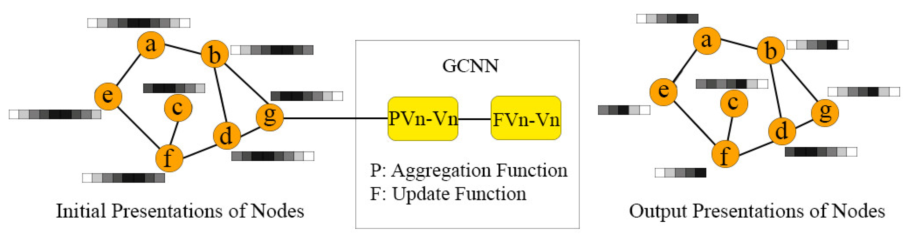
Graph Convolutional Neural Network
4. Research Model
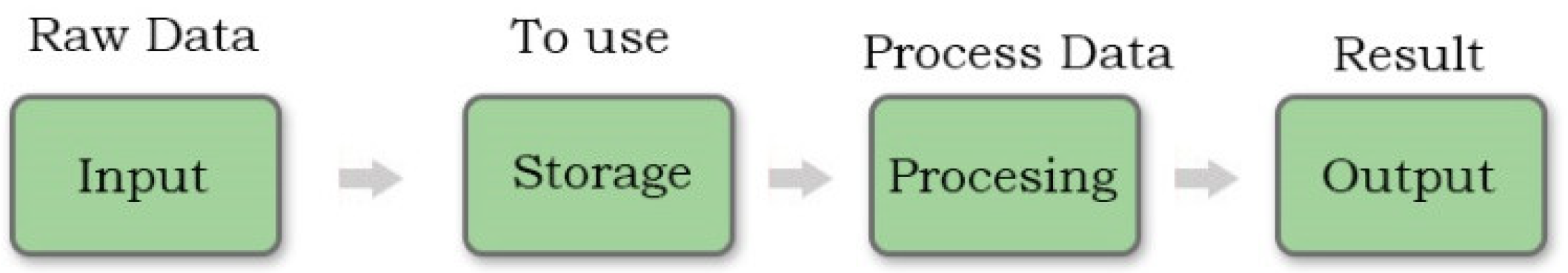
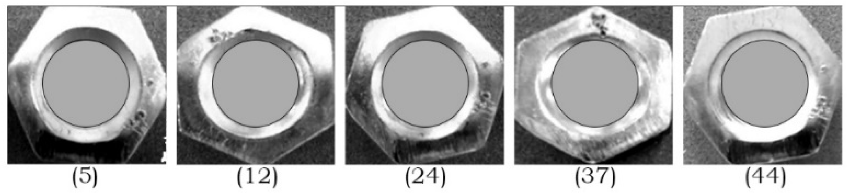
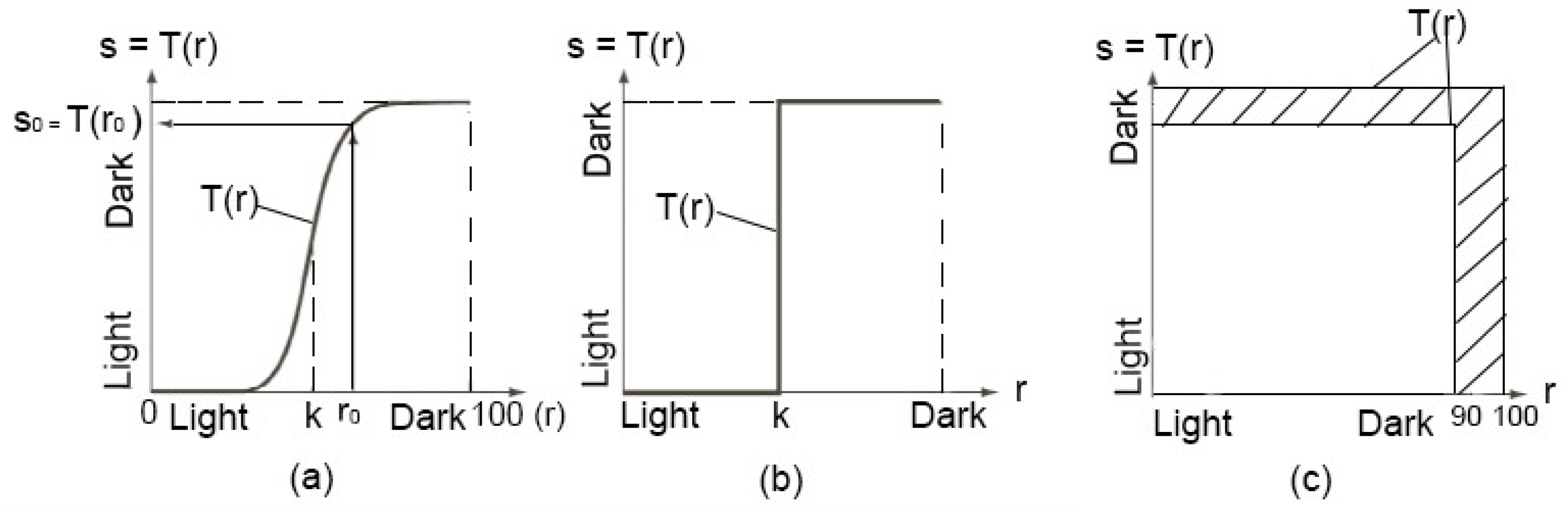
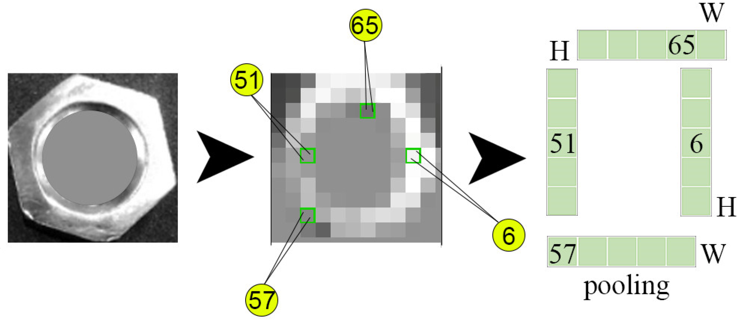
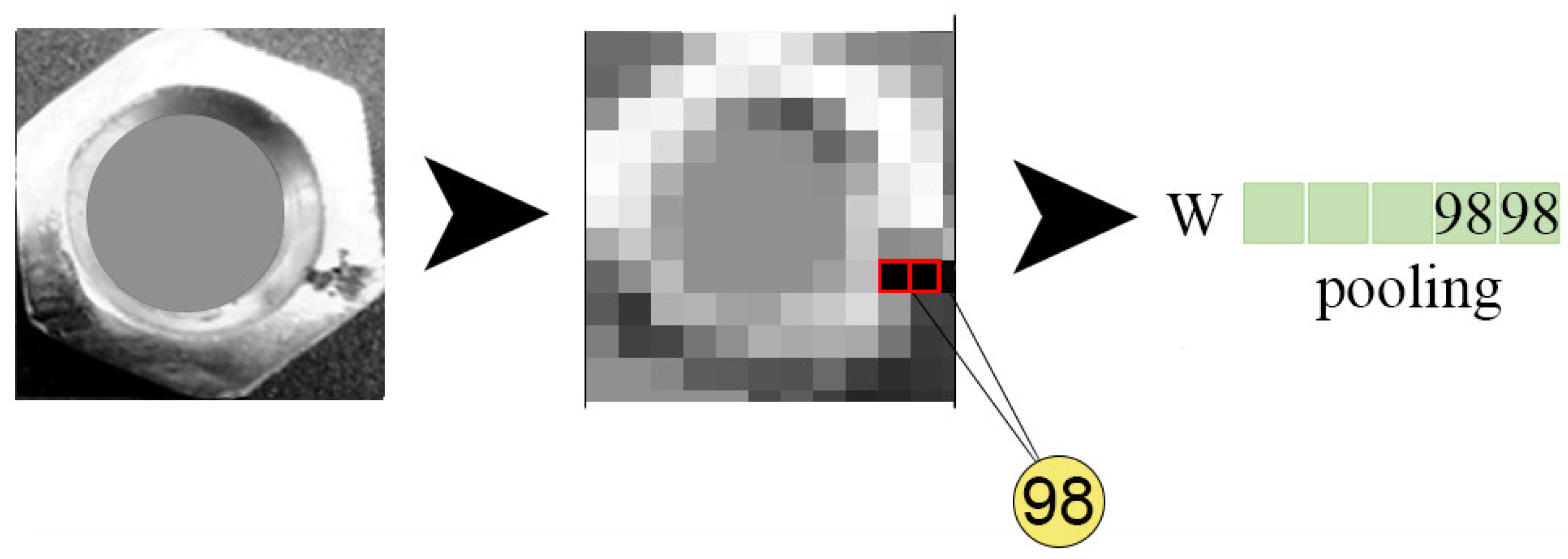
4.1. Image Processing
4.2. Hardware Build
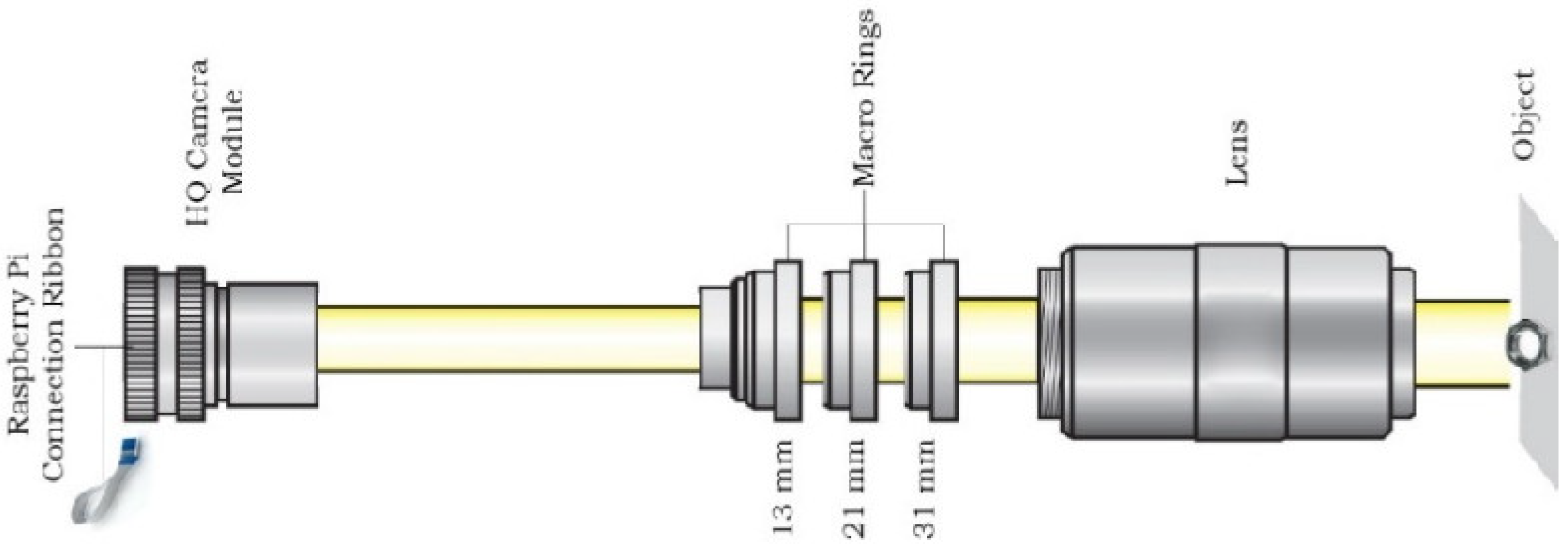
4.2.1. Camera Interface
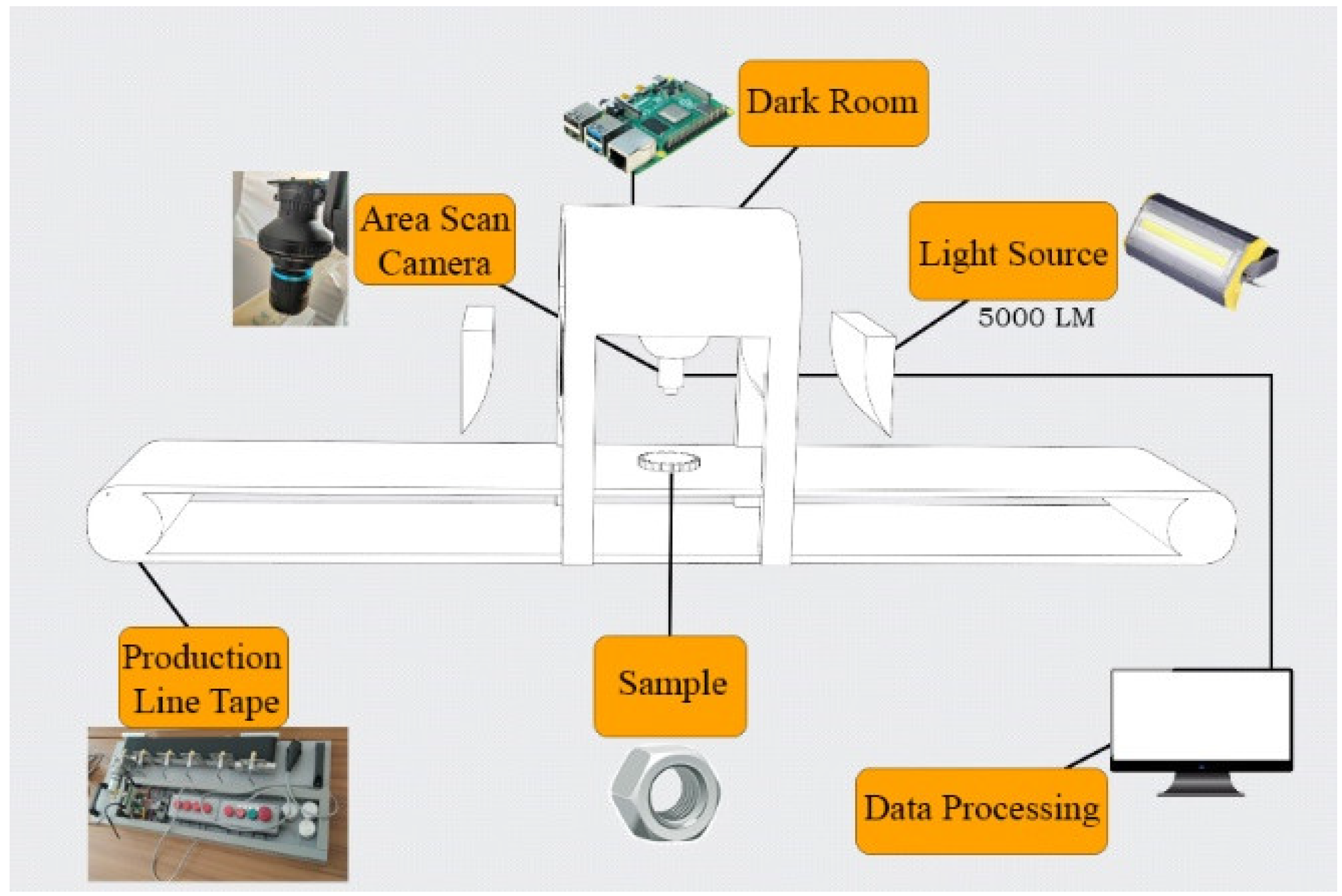
4.2.2. Model Defect Inspections Process
5. Procedures
Methodology
6. Evaluated Algorithm
7. Conclusions and Discussions
Author Contributions
Funding
Data Availability Statement
Conflicts of Interest
References
- Chen, H.; Pang, Y.; Hu, Q.; Liu, K. Solar cell surface defect inspection based on multispectral convolutional neural network. J. Intell. Manuf. 2020, 31, 453–468. [Google Scholar] [CrossRef]
- Du, W.; Shen, H.; Fu, J.; Zhang, G.; He, Q. Approaches for improvement of the X-ray image defect detection of automobile casting aluminum parts based on deep learning. NDT Int. 2019, 107, 102–144. [Google Scholar] [CrossRef]
- Ferguson, M.; Ak, R.; Lee, Y.T.T.; Law, K.H. Detection and segmentation of manufacturing defects with convolutional neural networks and transfer learning. Smart Sustain. Manuf. Syst. 2018, 2, 1007121126. [Google Scholar] [CrossRef]
- Lv, X.; Duan, F.; Jiang, J.J.; Fu, X.; Gan, L. Deep active learning for surface defect detection. Sensors 2020, 20, 1650. [Google Scholar] [CrossRef]
- Dalal, N.; Triggs, B. Histograms of oriented gradients for human detection. In Proceedings of the 2005 IEEE Computer Society Conference on Computer Vision and Pattern Recognition, CVPR 2005, San Diego, CA, USA, 20–26 June 2005. [Google Scholar] [CrossRef]
- Lin, T.Y.; Dollár, P.; Girshick, R.; He, K.; Hariharan, B.; Belongie, S. Feature pyramid networks for object detection. In Proceedings of the 30th IEEE Conference on Computer Vision and Pattern Recognition, CVPR 2017, Honolulu, HI, USA, 21–26 July 2017. [Google Scholar] [CrossRef]
- Wang, J.; Perez, L. The effectiveness of data augmentation in image classification using deep learning. arXiv 2017, arXiv:1712.04621v1. [Google Scholar]
- Perez, H.; Tah, J.H.M.; Mosavi, A. Deep learning for detecting building defects using convolutional neural networks. Sensors 2019, 19, 3556. [Google Scholar] [CrossRef]
- Krizhevsky, A.; Sutskever, I.; Hinton, G.E. ImageNet classification with deep convolutional neural networks. Commun. ACM 2017, 60, 84–90. [Google Scholar] [CrossRef]
- Awan, M.J.; Rahim, M.S.; Salim, N.; Mohammed, M.A.; Garcia-Zapirain, B.; Abdulkareem, K.H. Efficient Detection of Knee Anterior Cruciate Ligament from Magnetic Resonance Imaging Using Deep Learning Approach. Diagnostics 2021, 11, 105. [Google Scholar] [CrossRef]
- Hechtlinger, Y.; Chakravarti, P.; Qin, J. A generalization of convolutional neural networks to graph-structured data. arXiv 2017, arXiv:1704.08165v1. [Google Scholar]
- Lim, D.U.; Kim, Y.G.; Park, T.H. SMD Classification for Automated Optical Inspection Machine Using Convolution Neural Network. In Proceedings of the 3rd IEEE International Conference on Robotic Computing, I.R.C, Naples, Italy, 25–27 February 2019. [Google Scholar] [CrossRef]
- Yang, Y.; Pan, L.; Ma, J.; Yang, R.; Zhu, Y.; Yang, Y.; Zhang, L. A high-performance deep learning algorithm for the automated optical inspection of laser welding. Appl. Sci. 2020, 10, 933. [Google Scholar] [CrossRef]
- Lopac, N.; Hržić, F.; Vuksanović, I.P.; Lerga, J. Detection of Non-Stationary GW Signals in High Noise from Cohen’s Class of Time-Frequency Representations Using Deep Learning. IEEE Access 2022, 10, 2408–2428. [Google Scholar] [CrossRef]
- Lin, H.; Li, B.; Wang, X.; Shu, Y.; Niu, S. Automated defect inspection of L.E.D. chip using deep convolutional neural network. J. Intell. Manuf. 2019, 30, 2525–2534. [Google Scholar] [CrossRef]
- Jamshidi, A.; Roohi, S.F.; Núñez, A.; Babuska, R.; De Schutter, B.; Dollevoet, R.; Li, Z. Probabilistic Defect-Based Risk Assessment Approach for Rail Failures in Railway Infrastructure. IFAC-Pap. Online 2016, 49, 73–77. [Google Scholar] [CrossRef]
- Faghih-Roohi, S.; Hajizadeh, S.; Nunez, A.; Babuska, R.; De Schutter, B. Deep convolutional neural networks for detection of rail surface defects. In Proceedings of the International Joint Conference on Neural Networks, Vancouver, BC, Canada, 24–29 July 2016; pp. 2161–4407. [Google Scholar] [CrossRef]
- Bruna, J.; Sprechmann, P.; LeCun, Y. Super-resolution with deep convolutional sufficient statistics. In Proceedings of the 4th International Conference on Learning Representations, ICLR 2016, Conference Track Proceedings, San Juan, Puerto Rico, 2–4 May 2016. [Google Scholar]
- Atwood, J.; Towsley, D. Diffusion-convolutional neural networks. In Advances in Neural Information Processing Systems. 2016. Available online: https://proceedings.neurips.cc/paper/2016/hash/390e982518a50e280d8e2b535462ec1f-Abstract.html (accessed on 24 September 2022).
- Kipf, T.N.; Welling, M. Semi-supervised classification with graph convolutional networks. In Proceedings of the 5th International Conference on Learning Representations, ICLR 2017, Conference Track Proceedings, Toulon, France, 24–26 April 2017. [Google Scholar]
- Wu, Z.; Pan, S.; Chen, F.; Long, G.; Zhang, C.; Yu, P.S. A comprehensive survey on graph neural networks. arXiv 2019, arXiv:1901.00596v4. [Google Scholar] [CrossRef]
- Bruna, J.; Zaremba, W.; Szlam, A.; LeCun, Y. Spectral networks and deep locally connected networks on graphs. In Proceedings of the 2nd International Conference on Learning Representations, ICLR 2014, Conference Track Proceedings, Banff, AB, Canada, 14–16 April 2014. [Google Scholar]
- Li, R.; Wang, S.; Zhu, F.; Huang, J. Adaptive graph convolutional neural networks. In Proceedings of the 32nd AAAI Conference on Artificial Intelligence, AAAI 2018, New Orleans, LO, USA, 2–7 February 2018. [Google Scholar]
- Zhuang, C.; Ma, Q. Dual graph convolutional networks for graph-based semi-supervised classification. In Proceedings of the Web Conference 2018 World Wide Web Conference, W.W.W., Lyon, France, 23–27 April 2018. [Google Scholar] [CrossRef]
- Rathi, P.C.; Ludlow, R.F.; Verdonk, M.L. Practical High-Quality Electrostatic Potential Surfaces for Drug Discovery Using a Graph-Convolutional Deep Neural Network. J. Med. Chem. 2020, 63, 8778–8790. [Google Scholar] [CrossRef]
- Wang, Y.; Gao, L.; Li, X.; Gao, Y.; Xie, X. A New Graph-Based Method for Class Imbalance in Surface Defect Recognition. IEEE Trans. Instrum. Meas. 2021, 70, 1–16. [Google Scholar] [CrossRef]
- Wang, Y.; Gao, L.; Gao, Y. A new graph-based semi-supervised method for surface defect classification. Robot. Comput. Integr. Manuf. 2021, 68, 102083. [Google Scholar] [CrossRef]
- Villalba-Diez, J.; Schmidt, D.; Gevers, R.; Ordieres-Meré, J.; Buchwitz, M.; Wellbrock, W. Deep learning for industrial computer vision quality control in the printing industry 4.0. Sensors 2019, 19, 3987. [Google Scholar] [CrossRef]
- Wang, M.; Li, Y.; Zhang, Y.; Jia, L. Spatio-temporal graph convolutional neural network for remaining useful life estimation of aircraft engines. Aerosp. Syst. 2020, 4, 29–36. [Google Scholar] [CrossRef]
- Gilmer, J.; Schoenholz, S.S.; Riley, P.F.; Vinyals, O.; Dahl, G. Neural message passing for quantum chemistry. In Proceedings of the 34th International Conference on Machine Learning, Sydney, NSW, Australia, 6–11 August 2017; Volume 70. [Google Scholar]
- Schlichtkrull, M.; Kipf, T.N.; Bloem, P.; Van Den Berg, R.; Titov, I.; Welling, M. Modeling Relational Data with Graph Convolutional Networks. In Lecture Notes in Computer Science; Including subseries Lecture Notes in Artificial Intelligence and Lecture Notes in Bioinformatics; Springer: Berlin/Heidelberg, Germany, 2018. [Google Scholar] [CrossRef]
- Mou, L.; Lu, X.; Li, X.; Zhu, X.X. Nonlocal Graph Convolutional Networks for Hyperspectral Image Classification. IEEE Trans. Geosci. Remote Sens. 2020, 58, 8246–8257. [Google Scholar] [CrossRef]
- Jain, V.; Seung, H.S. Natural image denoising with convolutional networks. Advances in Neural Information Processing Systems. In Proceedings of the 2008 Conference NIPS, Vancouver, BC, Canada, 8–11 December 2008. [Google Scholar]
- Shilpashree, K.S.; Lokesha, H.; Shivkumar, H. Implementation of Image Processing on Raspberry Pi. Int. J. Adv. Res. Comput. Commun. Eng 2015, 4, 199–202. [Google Scholar] [CrossRef]
- Gonzalez, R.C.; Woods, R.E.; Masters, B.R. Digital Image Processing, Third Edition. J. Biomed. Opt. 2009, 14, 029901. [Google Scholar] [CrossRef]
- Zhang, J.; Kang, X.; Ni, H.; Ren, F. Surface defect detection of steel strips based on classification priority YOLOv3-dense network. Ironmak. Steelmak. 2020, 48, 547–558. [Google Scholar] [CrossRef]
- Zhou, Y.; Yu, L.; Zhi, C.; Huang, C.; Wang, S.; Zhu, M.; Ke, Z.; Gao, Z.; Zhang, Y.; Fu, S. A Survey of Multi-Focus Image Fusion Methods. Appl. Sci. 2022, 12, 6281. [Google Scholar] [CrossRef]
- Xu, Z.F.; Jia, R.S.; Liu, Y.B.; Zhao, C.Y.; Sun, H.M. Fast method of detecting tomatoes in a complex scene for picking robots. IEEE Access 2020, 8, 55289–55299. [Google Scholar] [CrossRef]


| Configuration of GCN Models | ||||||||||||||
|---|---|---|---|---|---|---|---|---|---|---|---|---|---|---|
| Gaussian Noise | Speckle Noise | |||||||||||||
| Monochrome | Histogram Equalization | Max. Rotation | Max. Verical Shift | Max. Horizontal Shift | Min. Scale | Max. Scale | Max. Vertical Shear | Max. Horizontal Shear | Max. Brightness | Min.Std Dev. | Max. Std Dev. | Min. Std Dev. | Max. Std Dev. | |
| Model 1 | yes | yes | 45 | 10 | 10 | 0.1 | 0.1 | 45 | 10 | 10 | 5 | 10 | 0.05 | 0.1 |
| Model 2 | yes | yes | 90 | 20 | 20 | 0.2 | 0.2 | 55 | 20 | 20 | 10 | 20 | 0.1 | 0.15 |
| Model 3 | yes | yes | 135 | 30 | 30 | 0.3 | 0.3 | 65 | 30 | 30 | 15 | 30 | 0.15 | 0.2 |
| Model 4 | yes | yes | 180 | 40 | 40 | 0.4 | 0.4 | 75 | 40 | 40 | 20 | 40 | 0.2 | 0.25 |
| Model 5 | yes | yes | 225 | 50 | 50 | 0.5 | 0.5 | 85 | 50 | 50 | 25 | 50 | 0.25 | 0.3 |
| Model 6 | yes | yes | 270 | 60 | 60 | 0.6 | 0.6 | 95 | 60 | 60 | 30 | 60 | 0.3 | 0.35 |
| Model 7 | yes | yes | 315 | 70 | 70 | 0.7 | 0.7 | 105 | 70 | 70 | 35 | 70 | 0.35 | 0.4 |
| Accuracy Comparisons for Metal Nut Images. Bold Numbers Indicate the Best Performance. | ||||||||||
|---|---|---|---|---|---|---|---|---|---|---|
| Class No. | Class Name | Model 1 | Model 2 | Model 3 | Model 4 | Model 5 | Model 6 | Model 7 | 2D CNN | YOLOv3 |
| 1 | Nut | 90.8816 | 75.9536 | 76.1821 | 72.9791 | 90.2698 | 88.9597 | 90.6628 | 87.9262 | 90.6145 |
Disclaimer/Publisher’s Note: The statements, opinions and data contained in all publications are solely those of the individual author(s) and contributor(s) and not of MDPI and/or the editor(s). MDPI and/or the editor(s) disclaim responsibility for any injury to people or property resulting from any ideas, methods, instructions or products referred to in the content. |
© 2023 by the authors. Licensee MDPI, Basel, Switzerland. This article is an open access article distributed under the terms and conditions of the Creative Commons Attribution (CC BY) license (https://creativecommons.org/licenses/by/4.0/).
Share and Cite
Balcıoğlu, Y.S.; Sezen, B.; Çerasi, C.C.; Huang, S.H. Machine Design Automation Model for Metal Production Defect Recognition with Deep Graph Convolutional Neural Network. Electronics 2023, 12, 825. https://doi.org/10.3390/electronics12040825
Balcıoğlu YS, Sezen B, Çerasi CC, Huang SH. Machine Design Automation Model for Metal Production Defect Recognition with Deep Graph Convolutional Neural Network. Electronics. 2023; 12(4):825. https://doi.org/10.3390/electronics12040825
Chicago/Turabian StyleBalcıoğlu, Yavuz Selim, Bülent Sezen, Ceren Cubukcu Çerasi, and Shao Ho Huang. 2023. "Machine Design Automation Model for Metal Production Defect Recognition with Deep Graph Convolutional Neural Network" Electronics 12, no. 4: 825. https://doi.org/10.3390/electronics12040825
APA StyleBalcıoğlu, Y. S., Sezen, B., Çerasi, C. C., & Huang, S. H. (2023). Machine Design Automation Model for Metal Production Defect Recognition with Deep Graph Convolutional Neural Network. Electronics, 12(4), 825. https://doi.org/10.3390/electronics12040825