Revisiting Homophily Ratio: A Relation-Aware Graph Neural Network for Homophily and Heterophily

Abstract

The graph neural network (GNN) is a type of powerful deep learning model used to process graph data consisting of nodes and edges. Many studies of GNNs have modeled the relationships between the edges and labels of nodes only by homophily/heterophily, where most/few nodes with the same label tend to have an edge between each other. However, this modeling method cannot describe the multiconnection mode on graphs where homophily can coexist with heterophily. In this work, we propose a transition matrix to describe the relationships between edges and labels at the class level. Through this transition matrix, we constructed a more interpretable GNN in a neighbor-predicting manner, measured the information that the edges can provide for the node classification task, and proposed a method to test whether the labels match the edges. The results show the improvement of the proposed method against state-of-the-art (SOTA) GNNs. We also obtain the following two results: (1) the poor performance of GNNs is highly relevant to the information of edges instead of heterophily, which is always considered the main factor resulting in the decline in performance; and (2) most benchmark heterophilic datasets exhibit the label-edge mismatch problem, leading them to become intractable

1. Introduction

Graph neural networks have recently emerged as a powerful tool for modeling graph data. Classic models such as GCN [1], GAT [2], SGC [3], and GraphSAGE [4] have a wide range of applications in graph-related tasks such as medical data [5,6], city traffic data [7,8], and wireless networks [9,10]; moreover, these models have achieved the effect of SOTA. Additionally, these models iteratively aggregate the features of neighboring nodes to update the representation of their own nodes. Researchers in [11] interpret it as a method for solving an optimization problem with neighborhood smoothing.

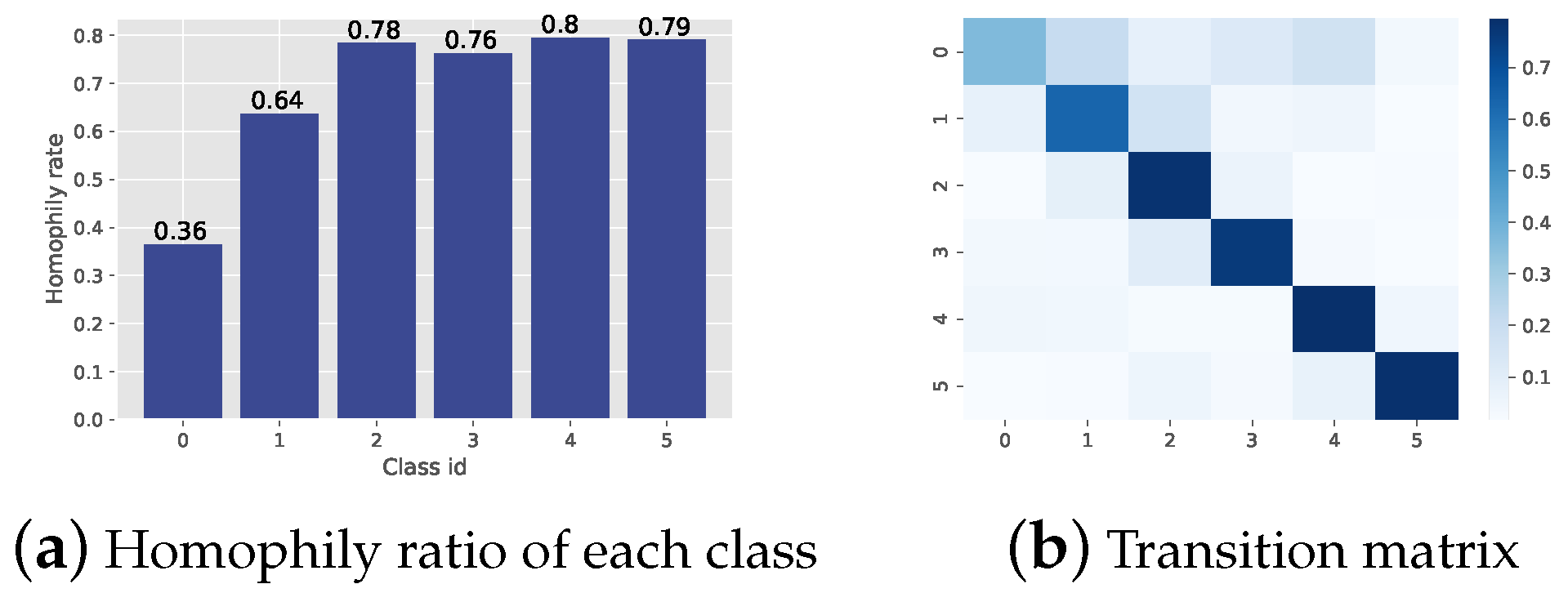
However, researchers have recently observed that nodes do not always tend to connect with nodes in the same class. This phenomenon is called heterophily, and there are also many cases in real scenes, such as heterosexual dating networks, protein interaction networks, and anomaly detection in systems that can be modeled as a graph [12,13]. Thus, the original neighbor smoothing strategy is no longer effective in theory. Therefore, in response to dealing with heterophilic graphs, researchers first defined the homophily ratio (HR) by the ratio of edges connecting nodes with the same class (intraclass edges) to total edges. Then, they proposed different strategies to process graphs guided by the homophily ratio. The definition of HR may have two fundamental problems that cause problems in processing graphs and even mislead research. First, the definition of the homophily ratio is based on the graph level, which ignores the multiple connection modes among classes, where some classes tend to connect with the same class while others may not. For instance, the homophily ratio of the commonly used dataset CiteSeer is 0.74, while as shown in Figure 1a, the HR of Class 1 is only 0.36. In this case, the design of GNNs guided by HRs may uniformly treat them as the same, which is not fair for Class 1. Therefore, it is difficult to define homophily in a scalar [14].

Second, a low homophily ratio is not the true factor that causes the GNN’s performance to decline. This phenomenon has been shown in many prior works, such as [14,15]. The level of the homophily ratio is not strictly linear with the performance of GNNs, and even in some cases of a low homophily ratio, the classic GNN still performs well. Therefore, a new quantitative index is needed to determine which data are bad or good and to indicate the reason affecting the GNNs. In this work, we proposed a transition matrix to describe the probability that a class of nodes may connect to another class of nodes through an edge, as shown in Figure 1b. Guided by this transition matrix and a simple assumption via stochastic equivalence, we first construct an interpretable model WTGNN that explicitly takes the multiconnection mode into consideration. In addition, each layer of the WTGNN can be explained through a neighbor prediction. Then, we quantify the information that edges can provide via entropy and find that it strongly affects the performance of GNNs through a series of experiments on synthetic and real graphs. Finally, we raise a label-edge mismatch argument that may cause low edge information and propose a corresponding method to test whether the labels match the edges on the graphs. Experimental results show that the most commonly used benchmark datasets treated as heterophilic graphs with poor performance have label-edge mismatch problems.

The main contributions are summarized as follows:

1. The label relationship between connected nodes is described via a transition matrix, and a highly interpretable model called the Walk and Transit Graph Neural Network (WTGNN) is derived. This model transforms the node classification problem into the aggregation of neighbor predictions and can solve constraint satisfaction problems. The calculation process of the model also conforms to the traditional graph neural network paradigm and is equivalent to prior work under certain conditions.

2. The information that edges provide via information entropy is measured, and it is found that it is closely related to the performance of GNNs rather than the homophily ratio. The lower the edge information entropy is, the better the performance of GNNs. Meanwhile, almost all real-world heterophilic graphs have high edge information entropy, which indicates that even though intractable graphs show low HR and high information entropy, we should address the problems caused by low edge information rather than low HR because it is the factor that truly affects the performance of GNNs.

3. The problem of mismatch between labels and edges is considered, and a method to test it is proposed. We first generate a large number of graphs with labels and edge relationships removed as null models and then calculate the probability that the edge information entropy of the generated graph is less than that of the original graph. If the probability is high, the graph has a label-edge mismatch problem. The edge of the randomly generated graph can provide more information with high probability. The experimental results show that almost all heterophilic datasets have label-edge mismatch problems.

The organization of this paper is as follows. In Section 2, related works are introduced. In Section 3, the definition of the problem, the assumptions required to derive the model, the definition of the transition matrix, and the related proposition are provided. In Section 4, the WTGNN based on neighbor prediction is introduced, the information entropy of the edge is calculated as an evaluation metric of the graph, and a method to test the label-edge mismatch problem is proposed. In Section 5, the features of the specifics of works are discussed. In Section 6, the performance of the WTGNN is tested, the correlation between edge information entropy and GNN performance is proven, and whether a label-edge mismatch problem exists in the benchmark datasets is determined through a series of experiments. In Section 7, concluding remarks are provided.

2. Related Work

GNNs. Graph neural networks show excellent data mining ability in semi-supervised node classification tasks because of their strong expression ability. An early version of GNN was proposed by extending the convolutional neural network of conventional meshes (such as images) to irregular meshes (such as graphics). Kipf and Welling [1] simplified the previous work and proposed a popular graph convolution network GCN. Velickovic et al. [2] and Hekumparampil et al. [16] introduced the attention mechanism into graph neural networks, which is also a classical graph neural network defined in the vertex domain. GraphSAGE [4], GIN [17], etc., have enhanced the aggregation function to capture information in graphs. The former can be applied to inductive learning on large-scale graphs. Furthermore, JumpingKnowledge Net [18] made use of the representation from the middle layer to make the GNN deeper. Similarly, APPNP [19] incorporated personalized PageRank into the aggregation function. Recently, GNN has been integrated with classical theories, such as fuzzy theory [13] and dynamic planning [20], resulting in corresponding work, such as FGNN [21] and DAGFM [21]. Our work is consistent with JumpingKnowledge and APPNP under certain conditions and this feature will be described in Section 5.2.

GNNs for heterophily. Recently, many studies on heterophily in graphs have emerged. First, H2GCN [22], Mix-hop [23], etc., alleviated the problem of heterophily by directly increasing the range of the receipt field and enhancing the weight of their own nodes during updates. H2GCN verifies that high-order neighbors contain more nodes with the same class when the labels of one-hop neighbors are conditionally independent of the label of the ego node. Following a similar idea, UGCN [24] introduces a multitype convolution to extract information from 1-hop and 2-hop and designs a discriminative aggregation to sufficiently fuse them to provide learning objectives. In addition, TDGNN [25] leverages tree decomposition to separate neighbors at different k-hops into multiple subgraphs and then propagates information on these subgraphs in parallel. GPR-GNN, APPNP, and other methods that expand the receipt field by stacking layers are also effective for mismatched maps. In the spectral domain, in contrast to Laplacian smoothing [26] and low-pass filtering [3] that approximate graph Fourier transformations on homophilic graphs, spectral GNNs on heterophilic graphs involve both low-pass and high-pass filters to adaptively extract low-frequency and high-frequency graph signals [27]. Typically, FAGCN [28] adopts a self-gating attention mechanism to learn the proportion of low-frequency and high-frequency signals. The other type of work is to guide neighbor aggregation by identifying the category of connected nodes. The representative works are GBK-GNN [29], GAM [30], GGCN [31], etc. They modeled homophily at the node level. Different messages are transmitted through the similarity between different nodes or the consistency of labels to strengthen the influence of the same class and weaken the influence of different classes. However, these studies were not focused on the description and modeling of the relationship between classes, and heterophily was regarded as the reason for the decline in GNN performance. However, both our experiment and the experiment in [15] provided negative examples.

3. Preliminaries

3.1. Notations and Problem Setting

An undirected graph $G=(V,E,X)$ where V and E denote nodes and edges in G, respectively. $X\in R^{n\times d}$ is the feature matrix of nodes. Each node $v_i$ has a label $Y_i\in \{y_1,y_2\dots y_m\}$, where c is the total number of labels. We let $Z_i=\pi \left(Y_i\right)\in R^{1\times m}$ indicate the label probability distribution of node $v_i$. ${\mathcal{N}}_k\left(i\right)$ denotes the node set that can exactly walk k steps to reach $v_i$ on the graph; for convenience, it is called the k-hop neighborhood in the next context. The random walk matrix is defined as $A=A{D}^{-1}$, where A is the adjacency matrix of G and D is the degree matrix, where $D_{ii}={\Sigma }_i{A}_i$.

The node classification task on G is defined as follows: Given an unlabeled subset $V_U$ of V, the GNN model shall use the information on the graph and provide the probability distribution $P(Z_i\mid G),v\in V_U$ to indicate in which class $v_i$ most belongs.

3.2. Homophily and Heterophily

Homophily or heterophily describes the preferences of nodes that tend to connect to nodes with the same or different classes. They are measured by the homophily ratio, which is calculated by

$$HR=\frac{1}{\left|V\right|}\sum _{i\in V}\frac{1}{|{\mathcal{N}}_1\left(i\right)|}\sum _{j\in {\mathcal{N}}_1\left(i\right)}{\mathbf{1}}_{y_i=y_j}$$

(1)

where $\left|V\right|$ is the number of nodes, $|{\mathcal{N}}_1\left(i\right)|$ is the size of the 1-hop neighborhood of Node i, and $\mathbf{1}$ is the indicator function. It calculates the average ratio of the same-class neighbor of each node. The smaller the HR is, the more heterophily the graph has. Therefore, it measures the homophily at the graph level and cannot reflect the complex connection preference of each class.

3.3. Assumption and Definitions

Assumption (Stochastic Equivalence). 

For any node u and v with the same class $y_j$, and any node $r,s$ that connects to u and v, it is assumed that $e_{u}r$ is independent of $Y_u$ and $Y_r$, and they satisfy the following equation:

$$P(Y_r=y_i\mid Y_u=y_j,e_{ur})=P(Y_s=y_i\mid Y_v=y_j,e_{vs})$$

(2)

Similar to the concept of stochastic equivalence in the stochastic block model (SBM) [32], it is assumed that nodes with the same class share the probability of having a neighbor of any certain class.

Definition 1 (Transition Matrix $C$). 

Given any node $u,v\in V,e_{uv}\in E$, and any label $y_i,y_j\in Y$, each element of the transition matrix C is defined as:

$$C_{ij}=P(Y_v=y_i\mid Y_u=y_j,e_{uv}),$$

(3)

According to the above assumption, $e_{uv}$ is independent of $Y_u$ and $Y_v$, and the equation holds for any $u,v$. It can be rewritten as $P(y_i\mid y_j)$ for convenience, and the transition matrix is:

$$C=\left[\begin{array}{ccc}P\left(y_1\mid y_1\right)& \cdots & P\left(y_1\mid y_m\right)\\ ⋮& \ddots & ⋮\\ P\left(y_1\mid y_m\right)& \cdots & P\left(y_c\mid y_m\right)\end{array}\right]$$

(4)

It can describe any connection mode on the graph and can be used to predict the labels of node neighbors according to the assumption. As Proposition 1 shows.

Proposition 1 (Neighbor Predicting). 

Given nodes $u,v$, edge $e_{uv}\in E$ and $Z_u$ is label probability distribution of node u, the label probability distribution of v is predicted by u as:

$$P_{z_u}\left(Z_v\right)=Z_{u}C$$

(5)

Equation (5) can be easily obtained from the total probability theorem. Since the prediction is independent of the neighbor node, the prediction can be performed for a k-hop neighbor node such as a Markov chain. Therefore, given v is a k-hop neighbor of node u, it can be predicted as:

$$P_{z_u}\left(Z_v\right)=Z_v{C}^k$$

(6)

Through this property, we build an interpretable, deep GNN, and it is equivalent to the classical GNNs under special conditions.

4. Proposed Method and Metrics

In this section, the proposed method is shown starting with an overview of the model design in the model construction part, following the training workflow with model details. Finally, the metrics for edge information and the label-mismatch problem are introduced.

4.1. Model Construction

The construction of the model is introduced from top to bottom. First, the goal of node classification task $P(Z_i\mid G)$ can be transformed into the aggregation of $P(Z_i\mid {\mathcal{N}}_k\left(v\right)$), and then $P(Z_i\mid {\mathcal{N}}_k\left(v\right))$ is decomposed into the aggregation of $P_{Z_j}\left(Z_i\right)$, and finally, the transition matrix is learned via a self-supervised fashion. C. A detailed introduction is as follows:

Given that G is a connected graph and K ≥ the diameter of G, the sum of the k-hop neighborhood of any node contains all nodes and edges in the graph G. Thus, the node classification task can be transformed into using k-hop neighborhoods to predict the node and can be written as:

$$\widehat{P}\left(Z_i\mid G\right)=E_{\alpha }\left[P(Z_i\mid {\mathcal{N}}_k\left(v\right))\right]=\sum _{k=0}^{k=K}{\alpha }_{k}P(Z_i\mid {\mathcal{N}}_k\left(v\right))$$

(7)

where ${\alpha }_k$ is the prior probability that measures the impact of each k-hop neighborhood on classification.

The next step is to calculate $P(Z_i\mid {\mathcal{N}}_k\left(v\right))$. Each k-hop neighborhood consists of the nodes that can walk to Node $v_i$ in the exact k step, and their predictions to $v_i$ are $Z_j{C}^k$. The random walk probability is used to average all predictions from ${\mathcal{N}}_k\left(v\right)$; thus, the probability estimation of v can be obtained as:

$$\widehat{P}\left(Z_i\mid {\mathcal{N}}_k\left(v\right)\right)=E_{{\widehat{A}}_{ij}}\left[P_{Z_j}\left(Z_i\right)\right]=\sum _{j\in \mathcal{N}\left(v\right)}{\widehat{A}}_{ij}^k{Z}_j{C}^k$$

(8)

In this case, Equation (7) rewritten in matrix level is:

$$\widehat{P}\left(Z\mid G\right)={\alpha }_k\sum _{k=0}^{k=K}{\widehat{A}}^{k}Z{C}^k$$

(9)

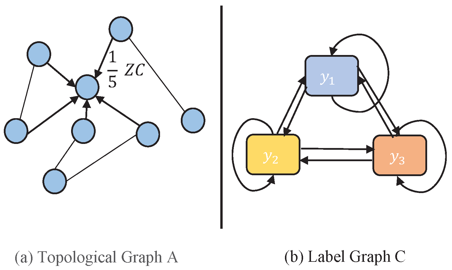
This Equation (8) indicates that each node receives the probability prediction from its k-hop neighborhood. Compared with GCN, SGC, APPNP, etc., nodes directly propagate and aggregate the information of neighboring nodes, and the proposed method aggregates the label information transited k steps via transition matrix C from its k-hop neighbor and weighted with the probability of random walk. Therefore, as shown in Figure 2, it can be explained as node random walks on two graphs: Node $v_j$ walks k steps in the topological graph $\widehat{A}$ to propagate its transited label (which is reflected in the equation ${\widehat{A}}^{k}Z$), and its label transits k steps on the label graph C (which is reflected in the equation $Z{C}^k$). Therefore, the proposed method is called the Walk and Transit GNN (WTGNN). In particular, if $\widehat{A}=D^{-1/2}\mathrm{A}{D}^{-1/2}$, then the probability that $v_j$ walks to $v_i$ is the same as the weight that $v_i$ accepts the transited label of $v_j$. Thus, the label propagation and aggregation C on the graph become a dual problem.

Meanwhile, the calculation of the transition matrix C should be performed. The inherent requirement of C is to predict neighboring nodes via edges and labels. Therefore, we use a self-supervised auxiliary task to solve it:

$$\begin{array}{c}\min \sum _i\sum _j{\widehat{A}}_{ij}{∥Z_i-Z_{j}C∥}_2^2\\ \mathrm{s}.\mathrm{t}.\sum _{j=0}^{j=c}{C}_{ij}=1,C>0,i=1,2\dots c\end{array}$$

(10)

The task can be seemed as solving $2\left|E\right|$ least square problem, where each node should predict its neighbor, and ${\widehat{A}}_{ij}$ is the weight for each problem.

So the whole model of WTGNN can be explained as solving the following problem:

$$\begin{array}{cc}& min-\sum _{i}ln{Y}_i\widehat{P}\left(Z_i\mid G\right)+\sum _{ij}{A}_{ij}{∥Z_i-Z_{j}C∥}_2^2\\ & \mathrm{where}\widehat{P}\left(Z_i\mid G\right)=\sum _{k=0}^{k=K}{\alpha }_k\sum _{j\in N\left(i\right)}{\widehat{A}}_{ij}^k{Z}_j{C}^k\\ & \mathrm{s}.\mathrm{t}.\sum _{k=0}^{k=K}{\alpha }_k=1\\ & \sum _{j=0}^{j=c}{C}_{ij}=1,C>0,i=1,2\dots m\end{array}$$

(11)

4.2. Training Process

Through the overall description of the model, the end-to-end model training process can be divided into three parts. The first part obtains the probability distribution of initial node labels, the second part trains the transition matrix, and the third part is the aggregation. The details are shown in Figure 3, and the parts are described as follows:

Part 1: Initialize the label distribution of nodes. As shown in Figure 3, the label distribution of nodes can be initialized through multilayer perception:

$$Z^{\left(0\right)}=softmax(WX+b)$$

(12)

Or it can even be calculated by an existing GNNslayer such as GCN [1]:

$$Z^{\left(0\right)}=softamx\left(\tilde{A}\sigma \left(\tilde{A}X{W}_1\right)X{W}_2\right)$$

(13)

Since the topology of a graph is not always trustworthy [33], it is a more generalized choice to use only feature information to obtain an initial evaluation. However, if the edges provide useful information, then using GNN is an option to obtain higher performance.

Part 2: Calculate the transition matrix. Since there is no way to obtain the estimated value of C directly from the label, C can only be solved through neighbor prediction tasks. We take the mean square error as the loss function:

$${\mathcal{L}}_{\mathrm{matrix}}\left(C\right)=\sum _i\sum _j{\widehat{A}}_{ij}{∥Z_i-Z_{j}C∥}_2^2$$

(14)

Part 3: Aggregation. The aggregation Equation (9) can be rewritten as a layer-by-layer convolution type:

$$Z^{\left(k\right)}=Z^{(k-1)}+\widehat{A}{Z}^{(k-1)}C$$

(15)

$$Z^{\left(final\right)}=[Z^{\left(0\right)},Z^{\left(1\right)},\dots ,Z^{\left(k\right)}]\left[\begin{array}{c}{\alpha }_0\\ {\alpha }_1\\ ..\\ {\alpha }_k\end{array}\right]$$

(16)

In each layer, the aggregating operation is equal to each node aggregates predictions from its k-hop neighbors weighted by the probability of random walk. The results of each layer $Z^{\left(k\right)}$ are integrated according to the influence coefficient ${\alpha }_k$ of different k hops. This step can also be regarded as a dense connection layer [34]. We take the cross-entropy function as the loss function:

$${\mathcal{L}}_{\mathrm{conv}}(\Theta ,\alpha )=-\sum _i{Z}_i^{\left(final\right)}ln{Y}_i,i\in {\mathcal{T}}_{\mathcal{V}}$$

(17)

where $\Theta$ is the parameter of MLP or GNN in the first part, ${\mathcal{T}}_{\mathcal{V}}$ are the labeled nodes. So the whole loss function is:

$${\mathcal{L}}_{\mathrm{total}}(\Theta ,C,\alpha )={\lambda }_1{\mathcal{L}}_{\mathrm{conv}}+(1-\lambda ){\mathcal{L}}_{\mathrm{matrix}}+{\parallel \Theta \parallel }_2$$

(18)

4.3. Proposed Measurement

Heterophily, which is a research direction of graph neural networks, is often considered a kind of graph that does not conform to the design of classical graph neural networks. Some recent studies [14,15,35] found through experiments that heterophily does not necessarily lead to a decline in the GNN performance, and there are still good or bad differences in heterophily. However, little work has been performed to propose a quantitative indicator that affects the performance of graph neural networks. In our work, we divide the graph into two types of data, node features, and edges, and consider that the performance of the GNN is affected by the information they provide.

Through the assumption of stochastic equivalence, we can calculate the entropy of edges ${\mathcal{H}}_E(G,C)$ which describes how many bits of information are still needed on average for a node to predict a connected node via an edge:

$$\begin{array}{cc}\hfill {\mathcal{H}}_E(G,C)& =\frac{1}{2N}\sum _i{\mathbf{D}}_i{h}_i\left({\pi }_{y_j}\left(y_i\right)\right)\hfill \\ \hfill & =\frac{1}{2N}\sum _i{\mathbf{D}}_i\sum _i-{\widehat{C}}_{ij}log{\widehat{C}}_{ij}\hfill \end{array}$$

(19)

$${\widehat{C}}_{ij}=\sum _i{e}_{ij}/\sum _i\sum _k{e}_{ik}$$

(20)

A high ${\mathcal{H}}_E(G,C)$ indicates that the edges provide little information for the node classification task, and vice versa.

4.4. Proposed Argument

However, what leads to this intractable graph data (bad heterophily with high edge information entropy) is a question that must be answered for further research. In this work, we consider an argument that edges cannot always reflect the relationship between the labels of connected nodes, which is called the label-edge mismatch problem. For example, in a lawyer network, each edge between two lawyers was built when they were assigned to handle the same case in a law firm. If the node/lawyer is labeled with a graduate school, obviously, the relationship between the edges and labels is weak. According to the content of the previous section, we propose a test method using the idea of the method of contradiction. It first assumes that the current edges and labels have the best matching relationship, that is, ${\mathcal{H}}_E(G,C)$ is assumed to be maximum, then a random perturbation graph $\tilde{G}$ is taken as a null model and its ${\mathcal{H}}_E(\tilde{G},\widetilde{C)}$ is calculated. Finally, the probability of ${\mathcal{H}}_E(\tilde{G},\tilde{C})\le {\mathcal{H}}_E(G,C)$ is calculated namely as follows:

$$\mathcal{M}-\mathrm{value}=P[{\mathcal{H}}_E(\tilde{G},\tilde{C})\le {\mathcal{H}}_E(G,C)]$$

(21)

It is worth noting that a low $\mathcal{M}$ value does not mean that the edges have provided the best description of the labels, but a high $\mathcal{M}$ value can prove that it does have a label-edge mismatch problem. We consider an example on multilabel graph data, the Lazega Lawyers [36] datasets, to show the different $\mathcal{M}$ values among different labels in the same structure, the results are shown in

Table 1. $\mathcal{M}$-value of different labels on the Lazega Lawyers network.

Data	Gender	Office	Practice	School
Cowork	0.12	0.04	0.3955	0.365
Friendship	0.15	0.045	0.39	0.355
Advice	0.09	0.015	0.375	0.38

.

In the Lazega lawyer network, there are three subgraphs constructed according to different relationships. Each lawyer has multiple types of labels, such as gender, graduation school, office location, and practice. If 0.1 is taken as the significance level, it is easy to find in Table 1 that the relationship between the graduation school, practice, and the network constructed according to friendship, advice, and cowork is weak.

5. Discussion

5.1. Generalization of Proposed Model

WTGNN aggregates the probability estimates from neighbors in the label space, which is highly interpretable; however, it also restricts its expression ability. Because labels may be determined by multiple unobservable hidden labels, such as hidden Markov chains, the relationship between observed labels may not have good regularity. Therefore, in order to further enhance the expression ability of WTGNN, we need to find a function $\Phi$ to generate the hidden labels $H:\{h_1,h_2\dots h_{m\prime }\}$, and a function $\varphi$ satisfying $\{h_1,h_2\dots h_{m\prime }\}\to \{y_1,y_2\dots y_m\}.$ Then, the WTGNN is equal to:

$$\begin{array}{c}{H}^{\left(0\right)}=\Phi (A,X)\\ H^{\left(final\right)}={\alpha }_k\sum _{k=0}^{k=K}{\widehat{A}}^k{H}^{\left(0\right)}{C}^k\\ \widehat{P}(Z\mid G)=\varphi \left(H^{\left(final\right)}\right)\end{array}$$

(22)

where C$\in R^{m\prime \times m\prime }$. $\Phi$ can be implemented by GNN or MLP, and $\varphi$ can also be implemented by MLP. It should be noted that the activation function of their last layer needs to use softmax to obtain the probability distribution of hidden labels. Its training process is the same as the original version.

5.2. Equivalence to Prior Work

If let $C=\mathbf{I}$, $\mathbf{I}$ is the identity matrix. That is assuming all nodes are connected with the same class. Then, WTGNN = ${\alpha }_k{\sum }_{k=0}^{k=K}{\widehat{A}}^{k}Z$, and is equivalent to a k term polynomial filter on a graph where the Laplace matrix L is $\widehat{A}$ and polynomial coefficient is ${\alpha }_k$. In this case, ChebyNet [37] is similar to our model. Furthermore, if let ${\alpha }_k=\beta {(1-\beta )}^k$ and the last term ${\alpha }_K={(1-\beta )}^K$, then WTGNN is equal to the Personalized PageRank (PPR) [19]. If let ${\alpha }_k=1$ then it is the same that of the SGC. Therefore, the main differences between the proposed method and typical label-aggregating GNNs are whether aggregate transited labels have a learnable layer influence coefficient $\alpha$. The feature-aggregating GNNs, such as JKNET [18], which aggregates the outputs of different GCN layers, are similar to the generalized WTGNN, but each layer of JKNET has a learnable weight matrix that should be trained.

5.3. Complexity

Compared with classical GNNs, WTGNN has fewer parameters and is invariant with layers. Only $d\times m+m^2+k$ parameters need to be trained during gradient descent, where d is the dimension of the node feature, and m is the number of classes. Before discussing time and space complexity, we assume that the adjacency matrix A and node feature matrix X are sparse matrices. For time complexity, the auxiliary task to train transition matrix C is $O\left(2m^2\right|E\left|\right)$. If MLP is chosen to initialize the probability distribution $Z^{\left(0\right)}$, the overall time complexity of WTGNN is $O(mn+2|E|m^2+nnz\left(X\right))$, if the GCN is chosen as the initializer, the overall time complexity is $O(n^2+2|E|m^2+nnz\left(X\right))$. The overall space complexity is $O\left(\right|E|+mn+m^2+nnz\left(X\right))$.

We show the average running time per epoch (ms)/average total running time (s) under different sizes of real-world datasets, and we summarize the results in

Table 2. Efficiency on selected real-world benchmark datasets.

	Cora	PubMed	Chameleon	Texas
GPRGNN	17.62 ms/3.74 s	20.19 ms/5.53 s	16.74 ms/3.40 s	17.56 ms/3.55 s
GCN	9.25 ms/1.86 s	14.11 ms/4.17 s	13.83 ms/2.79 s	10.22 ms/2.06 s
GAT	14.78 ms/3.42 s	21.52 ms/6.70 s	16.63 ms/3.63 s	15.50 ms/3.13 s
MLP	4.14 ms/0.92 s	5.43 ms/2.86 s	5.33 ms/2.77 s	2.86 ms/2.09 s
WTGNN(ours)	9.68 ms/1.95 s	16.51 ms/4.52 s	15.32 ms/3.06 s	12.74 ms/2.64 s

. Model training is performed on an Nvidia Tesla V100 GPU with 16 GB of memory. The maximum RAM consumption is not more than 1.2 GB.

5.4. HR and Edge Information Entropy

HR provides a description of how the nodes are connected at the graph level. A high HR indicates that most of the same nodes in the graph tend to be connected, while a low HR does not indicate that nodes with different nodes tend to be connected. There is also a case in which the distribution of connections in each class tends to be distributed uniformly, that is, there is no particular preference for the node connections. Experiments and prior works [15,29] show that graph neural networks are good at handling graphs with particular connecting preferences. In this work, we transform the graph neural network processing node classification problem into the aggregation of neighbor node predictions, which are based on the probability distribution of node connections. The more uniform the distribution is, the worse the prediction performance, indicating poor quality. High edge information entropy means that most node distributions are very close to a uniform distribution and are difficult to process by the graph neural network. The specific meaning of low and high HR and edge information entropy are summarized in

Table 3. Comparison between homophily ratio (HR) and edge information entropy (${\mathcal{H}}_E(G,C)$).

	Connecting Preference		Graph Quality
	The Same Class	Particular Different Class	Good	Poor
High HR	✓	×	✓	×
Low HR	×	×	×	×
High ${\mathcal{H}}_E(G,C)$	×	×	×	✓
Low ${\mathcal{H}}_E(G,C)$	×	×	✓	×

.

5.5. Prior Work of the Argument

Graph-structured data contain two kinds of data: The features of nodes and edges. Therefore, proposing and verifying the label-edge mismatch problem is a category of verifying data-label correlations. Data-label correlation is an important research direction in feature selection in machine learning. Many studies [38,39,40] have shown that if the correlation between data and labels is not high, the performance of the model will be severely limited. Furthermore, we are not the first study to show a weak correlation between the edges and labels of a skeptical graph. In [41], the researchers proposed that labels (or metadata) be used as ground truths to test whether the performance of community detection algorithms is unreasonable in some cases and proposed a test method. Similarly, we use a similar idea to test the mismatch between labels and edges in node classification tasks.

6. Experiments

In this section, we evaluate the proposed WTGNN with a node classification task on benchmark datasets, explore the effects of HR and the edge information entropy on the GNN performance, and test whether the heterophilic datasets in the benchmark suffer from the label-edge mismatch problem.

6.1. Data Description

Experiments are performed on nine datasets from PyTorch-Geometric [42], which are commonly used in graph neural network literature. We use a public data split provided by [43], the nodes of each class are 48%, 32%, and 20% for the training, validation, and testing sets, respectively. An introduction to the datasets is presented in

Table 4. Data Statistics.

Dataset	Homophily Ratio	Nodes	Edges	Classes
Texas	0.11	183	295	5
Wisconsin	0.21	251	466	5
Actor	0.22	7600	26,752	5
Squirrel	0.22	5201	198,493	5
Chameleon	0.23	2277	31,421	5
Cornell	0.3	183	280	5
Citeseer	0.74	3,327	4676	7
PubMed	0.8	19,717	44,327	3
Cora	0.81	2708	5278	7

. All benchmark datasets presented here are similar to graph-structured data in the electronic realm, such as wireless networks, and the implemented model can be easily generalized to the electronic realm.

Cora, CiteSeer and PubMed [44] are citation network-based datasets. In these datasets, nodes represent papers, and edges represent citations of one paper by another. The node features are the bag-of-words representation of papers, and the node labels denote the academic topic of a paper. Since these citation datasets have a high homophily ratio, they are considered homophily datasets.

Wisconsin, Cornell, and Texas are subdatasets of WebKB collected by Carnegie Mellon University. In these datasets, the nodes represent web pages, and the edges represent hyperlinks between them. The node features are the bag-of-words representation of web pages. The task is to classify the nodes into one of the following five categories: Student, project, course, staff, and faculty.

Actor [43] is the actor-only induced subgraph of the film– director–actor–writer network. Each node corresponds to an actor, and the edge between two nodes denotes co-occurrence on the same Wikipedia page. Node features correspond to some keywords on Wikipedia pages. The task is to classify the nodes into five categories in terms of words of actor’s Wikipedia.

Chameleon and Squirrel [45] are two page–page networks on specific topics in Wikipedia. The nodes represent web pages, and the edges are mutual links between the pages. The node features correspond to several informative nouns on Wikipedia pages. The labels of the nodes are five categories in terms of the number of the average monthly traffic of the web page.

6.2. Baselines Description

We compare our model with five baselines including two classic GNNs, an attribute-only based MLP, and two GNN-based SOTA methods aiming to analyze heterophilic graphs.

• MLP is a basic multilayer perception.
• GCN [1] is a semisupervised graph convolutional network model which learns node representations by aggregating information from neighbors.
• GAT [2] is a graph neural network model that uses an attention mechanism to aggregate node features.
• H2GCN [22] is a graph neural network designed for heterophily that combines ego and neighbor-embedding separation, higher-order neighborhoods, and a combination of intermediate representations,
• GPR-GNN [14] tried to obtain more valuable information by assigning signed weights to different layers.

6.3. Parameter Settings

For the baselines, we use their default parameter settings as they often lead to the best results. For our proposed method, we use the Adam [46] optimizer and set the number of hidden labels to {16, 32}, set the regularization term to {$1\times {10}^{-5},1\times {10}^{-6}$}, and the learning rate is chosen from {0.01, 0.05}. Set the balance parameter of loss $\lambda$ to 0.5, dropout ratio to 0.5, and learning rate to { 0.01, 0.05}. The initialization part is a 1-layer MLP with softmax activation for all datasets. In the aggregation part, the number of layers k is searched between 5 to 10 for all datasets, and we use the $\widehat{A}=D^{-1/2}A{D}^{-1/2}$ as a random walk matrix. Model training is performed on Nvidia Tesla V100 GPU with 16 GB memory.

6.4. Experimental Result

This section aims to evaluate the proposed WTGNN with node classification task on benchmark datasets and design experiments to explore how HR and edge information entropy affects GNN performance, and test whether the heterophilic datasets in the benchmark exist in label-edge mismatch problems.

6.5. Experiment on Node Classification

The results are shown in

Table 5. Mean accuracy(%) ± stdev over different data splits.

Method/Dataset	Texas	Wisconsin	Squirrel	Chameleon	Actor	Cornell	Citeseer	Cora	PubMed
HR	0.11	0.21	0.23	0.22	0.22	0.3	0.74	0.81	0.8
MLP	82.7 ± 6.19	85.29 ± 3.61	33.35 ± 1.24	48.20 ± 2.63	35.76 ± 0.98	81.08 ± 2.52	69.58 ± 2.31	74.14 ± 1.40	86.38 ± 0.61
GCN	58.38 ± 4.45	59.80 ± 6.90	36.89 ± 1.34	59.82 ± 2.57	30.26 ± 0.79	57.03 ± 4.67	76.68 ± 1.64	87.28 ± 1.26	87.38 ± 0.66
GAT	58.38 ± 4.45	55.29 ± 8.71	30.62 ± 2.11	54.69 ± 1.95	26.28 ± 1.73	58.92 ± 3.32	75.46 ± 1.72	82.68 ± 1.80	84.68 ± 0.44
H2GCN	84.86 ± 6.77	86.67 ± 4.69	36.42 ± 1.89	57.11 ± 1.58	35.86 ± 1.03	82.16 ± 4.80	77.07 ± 1.64	86.92 ± 1.37	88.78 ± 0.53
GPRGNN	84.59 ± 4.37	88.23 ± 1.96	29.45 ± 1.27	69.48 ± 1.97	39.30 ± 0.28	81.08 ± 3.46	75.12 ± 1.98	86.70 ± 1.03	87.38 ± 0.63
WTGNN	87.29 ± 5.67	89.41 ± 2.83	45.02 ± 1.61	67.98 ± 1.30	38.68 ± 0.09	82.70 ± 2.76	79.10 ± 1.45	89.29 ± 1.18	88.99 ± 0.33

Best results are in bold fonts.

, where the best results are in bold fonts. The proposed method achieved the best performance on seven of the nine datasets and the second-best performance on the remaining dataset. Considering the seven datasets, our WTGNN is on average 2.86%, 1.34%, 23.61%, 0.65%, 2.6%, 2.3%, and 0.23% more accurate than GCN, H2GCN, GPRGNN on Texas, Wisconsin, Squirrel, Cornell, Citeseer, Cora and PubMed, respectively. Specifically, on the Chameleon, Actor, and WebKB datasets, H2GCN and GPRGNN both show an improvement compared with the ordinary GCN, which shows the effectiveness of the heterophily design. However, on the Squirrel dataset, the GCN model exceeds the H2GCN and GPRGNN designed for heterophily, indicating that this HR-based design cannot cover all cases. However, our method shows a good generalization performance on almost all datasets, which verifies the express ability of the proposed transition matrix.

6.6. Experiment on Information Entropy of Edge

To test the impact of ${\mathcal{H}}_E(G,C)$, we should show its relationship with the accuracy of GNNs minus two-layer MLPs, which can remove the influence of the features provided by information nodes. WTGNNs and GCNs are evaluated on synthetic datasets generated by cSBM [47] and real-world benchmark datasets, and both have different levels of the homophily ratio. Synthetic datasets can facilitate analyses based on ideal conditions and can eliminate the impact of node features on the performance to the maximum extent, letting us focus only on the influence of the connection mode. The result is demonstrated in Figure 4, and the following conclusions can be determined through their impact on the performances GNNs:

First, by comparing (a) and (b), the improved performance of graph neural networks has a significant negative correlation with edge information entropies but has no linear relationship with the homophily ratio on synthetic datasets. In real datasets, as shown in (c) and (d), the improved performance also does not show a significant linear relationship with HR. However, there is basically a negative relationship with edge information entropy, except for chameleon and squirrel. This may be because the labels of the two datasets are not discrete but are continuous web traffic divided into different categories, and the transition matrix is more appropriate for describing the mapping relationship between labels.

Second, in the case of an extremely low homophily situation, the classic GCN can still perform well, as (a) shows. The reason is that in this case, the weight matrices of GCNs can capture the relationship between the labels of connected nodes because there is a significant mapping relation between them, even if an opposite effect occurs. The proposed WTGNN captures this relationship through an auxiliary task and uses it to classify nodes. If edges provide more information, the classification performance would be good, and vice versa. Therefore, when the label distribution of connected nodes tends to be uniform, the amount of information it provides is the least, and the performance of all GNNs is also the worst; in this case, the edge information entropy is $\approx 1$.

Finally, the WTGNN can maintain the performance of MLP compared with GCN, and enhance the utilization of structural information because its curve is always above 0 in all datasets.

6.7. Experiment on Label-Edge Mismatch Problem

We examine the $\mathcal{M}$ value on commonly used benchmark datasets, and the results are shown in

Table 6. $\mathcal{M}$-value, homophily ratio, and edge information entropy of benchmark dataset.

Dataset	$\mathcal{M}$-Value	HR	Entropy
Cora	0.074	0.81	0.391
PubMed	0	0.8	0.558
CiteSeer	0.002	0.74	0.520
Cornell	0.178	0.3	0.740
Chameleon	0.727	0.23	0.946
Squirrel	0.252	0.22	0.972
Actor	0.989	0.22	0.976
Wisconsin	0.075	0.21	0.735
Texas	0.935	0.11	0.709

. To better clarify the relationship between the heterophily and the $\mathcal{M}$-value, we set HR = 0.5 as the discriminant for the homophily and heterophily and take M-value = 0.1 as the significance level for the label-edge mismatch problem. As shown in Figure 5, the $\mathcal{M}$ value of five of the six heterophilic datasets is higher than 0.1, which indicates that they have a label-edge mismatch problem. This demonstrates that these datasets may be labeled inappropriately, such as in the Lazega Layers network being only labeled with the graduate school, which cannot reflect their relationship with co-workers. Alternatively, the edges do not describe the relationship between labels. For example, the lower $\mathcal{M}$-value of Actor indicates that using the co-occurrence to build edges is of little help to actor classification. GNNs usually have a low accuracy on these low $\mathcal{M}$-value datasets (except WebKB datasets, in which the node features provide much information for classification). Therefore, when evaluating graph-structured data, we should not only evaluate the relationship between labels and node features but also consider the relationship between edges and labels in nodes. Compared with the homophily ratio, the entropy of the edge can describe the information that edges provide, while the $\mathcal{M}$-value can test the problem behind the dataset.

6.8. Ablation Study

6.8.1. Number of Layers

The performance of the WTGNN under different layers is tested and shown in Figure 6. In our method, the kth layer represents the aggregation of the probability estimates from the k-hop neighborhood. Figure 6 shows that the WTGNN basically achieves the optimal results when k = 5 and k = 6. This coincides with the six-degree separation theory [48]. When k = 6, the WTGNN aggregates information from almost the whole map. After layer 6, in contrast to that of the traditional GCN, its performance does not decline sharply but can remain at a good level. GCNs will be excessively smooth after 2–3 layers in homophilic datasets. This is because the layer coefficient alpha can balance the credibility of the probability estimates of each k-hop neighborhood, thus alleviating the problem of oversmoothing in the GNN.

6.8.2. Auxiliary Task and Layer Influence Coefficient

The extent to which self-supervised auxiliary tasks and the layer influence coefficient $\alpha$ can influence the proposed method is explored in this section. Ablation experiments are performed in which only one feature is removed at a time and compared with the original WTGNN. Removing alpha means using the average of each layer to output the result, and removing ancillary tasks means that the transition matrix C is completely optimized by the loss function of the classification task. The results are shown in Figure 7. Both have a greater impact on the performance of the WTGNN, and the two designs have a greater improvement on the heterophilic data than homophilic data. The layer influence coefficients have a greater impact. The first reason is that WTGNN also uses neighbor prediction to handle node classification tasks, which is similar to the auxiliary tasks of neighbor predictions. The second reason is that layer influence coefficients can learn the hard-to-predict effects of different hop neighborhoods.

6.8.3. Initialize Method

The impact of two different initialization labels/hidden labels on the nine datasets with 10-fold different splits is tested in this section. The MLP denotes the use of a 1-layer MLP with softmax as the activation function to output soft labels, as shown in Equation (12). The GCN means using 1 layer of the graph convolution layer, as shown in Equation (13), which also uses softmax to output soft labels. The result is shown in

Table 7. Performance under different initial methods.

Dataset Type	Dataset	Initial Method
		WTGNN-MLP	WTGNN-GCN
Heterophily	Texas	87.29 ± 5.67	63.57 ± 5.70
	Wisconsin	89.41 ± 2.83	64.31 ± 4.27
	Chameleon	67.98 ± 1.30	57.01 ± 2.32
	Actor	38.68 ± 0.09	35.36 ± 1.09
	Squirrel	45.02 ± 1.61	38.24 ± 0.85
	Cornell	82.70 ± 2.76	51.89 ± 4.32
Homophily	Citeseer	78.19 ± 1.45	77.35 ± 1.92
	PubMed	88.99 ± 0.72	87.96 ± 0.27
	Cora	89.29 ± 1.18	89.56 ± 1.36

Better results are in bold fonts.

and the better results are in bold fonts. On heterophilic datasets that also have a high edge information entropy, initialization with GCNs can result in dramatic performance degradation. For example, on Chameleon datasets, performance decreases by 15.3%, while on Cornell, performance decreases by 38.06%. Not only do the edges not provide valid information, but they also mislead the accuracy level of soft labels, which can affect the training of the transition matrix C. Therefore, using GCN as an initialization tag function on such datasets is not an ideal choice. On datasets where labels and edges match, such as Cora, it has the smallest edge information entropy and the highest HR and taking GCN as an initialization function can outperform the MLP. In general, using the MLP as an initialization function is adequate for most situations and is not susceptible to the edges.

7. Conclusions

In this work, we use the stochastic equivalence assumption to describe the relationship between the labels of connected nodes in graph data, which can more accurately describe the connection modes on discrete graphs than the homophily ratio. With this assumption, we transform the node classification problem into a k-hop neighbor prediction problem and construct an interpretable model, WTGNN. The experimental results on nine benchmark datasets demonstrate the superiority of the proposed model, which is suitable for both homophily and heterophily. In addition, we provide a measurement of the information that edges can provide to the node classification task called edge information entropy and find that high edge information entropy is the main factor contributing to the performance degradation of GNNs, instead of a low homophily ratio. Furthermore, we raise an argument that the label-edge mismatch problem leads to intractable data and develop a test method for the problem. The experimental results show that this problem exists in five of the six heterophilic datasets. That means although researchers have theoretically completed the design for heterophily, it is not heterophily that truly makes the dataset difficult to process; thus, more and deeper problems remain to be explored and solved. In the future, WTGNN and related test methods can be further extended to networks in the electronic field, such as evaluating the reliability of wireless networks and electronic communication networks.