Prior-Driven NeRF: Prior Guided Rendering

Abstract

Neural radiation field (NeRF)-based novel view synthesis methods are gaining popularity. NeRF can generate more detailed and realistic images than traditional methods. Conventional NeRF reconstruction of a room scene requires at least several hundred images as input data and generates several spatial sampling points, placing a tremendous burden on the training and prediction process with respect to memory and computational time. To address these problems, we propose a prior-driven NeRF model that only accepts sparse views as input data and reduces a significant number of non-functional sampling points to improve training and prediction efficiency and achieve fast high-quality rendering. First, this study uses depth priors to guide sampling, and only a few sampling points near the controllable range of the depth prior are used as input data, which reduces the memory occupation and improves the efficiency of training and prediction. Second, this study encodes depth priors as distance weights into the model and guides the model to quickly fit the object surface. Finally, a novel approach combining the traditional mesh rendering method (TMRM) and the NeRF volume rendering method was used to further improve the rendering efficiency. Experimental results demonstrated that our method had significant advantages in the case of sparse input views (11 per room) and few sampling points (8 points per ray).

1. Introduction

Early neural radiation field (NeRF)-based models [1,2,3,4] used dense images as input, stored the radiation field and density of the scene in the multilayer perceptron (MLP) through training, and synthesized novel views through volumetric rendering [5]. Practically, there are several problems with this method. First, early NeRF-based models only used RGB values to determine the correlation information between images, and the volume rendering function was used to indirectly guide the network model in estimating the correct depth information and RGB values, which required dense images to help the network model to overcome the under/overfitting problem. Densely sampling images of a scene, particularly in outdoor spaces, is inefficient. Zhang et al. [6] decomposes a scene into 3D neural fields of surface normals, albedo, BRDF, and shading, which allows for applications such as free-viewpoint relighting and material editing. In addition, the method simplifies the volume geometry to a single surface and the light source visibility can be computed with a single MLP query, which allows for improved rendering efficiency. Second, early NeRF-based models used a dense sampling mode that approximately covered the entire local space to address the ambiguity and uncertainty in novel viewpoints. However, such a sampling mode imposes a significant overhead on hardware storage. A dataset of this size, consisting of 100 × 1080 × 720 pixel images and 128 sampling points per pixel, can yield approximately ten billion sampling points. Such a high data processing demand causes a significant hardware burden, limiting the rendering range and speed of these methods. DS-NeRF [7] helps the model to be trained by introducing a depth loss function, which reduces the number of input images required. DS-NeRF adds depth loss to guide the MLP in training, but still requires densely sampled points in prediction. ReLU Fields [8] uses explicit density grids with spherical harmonics for color processing, while introducing ReLU as the activation function to speed up model convergence. FastNeRF [9] improves rendering efficiency by compactly caching depth radiation maps at each location in space. Despite the efficiency of these methods, higher rendering quality cannot be achieved with sparse inputs. Yuan et al. [10] enhanced the quality of novel views by reconstructing the scene using depth information and pre-training a model with renderings of the scene. Such a method allows for better novel views under sparse input conditions.

Recently, some researchers [11,12] have started to experiment with introducing depth priors to the NeRF training process to aid in better network model convergence and to address the problems of slow training and dense image requirements caused by insufficient constraints. These methods mainly aid NeRF in training in two parts: (1) In the sampling mode, the original NeRF uses a hierarchical sampling method to increase the sampling rate in the area that may be the surface of the object, improving the accuracy. However, sampling the rays in most areas of the three-dimensional space that are not on the object’s surface would be resource intensive. The most recent method [13] obtains depth priors using the structure from motion algorithm (SFM) for sparse reconstruction and uses them to guide the model sampling decisions during model training. (2) For the loss function, because the original NeRF only uses RGB as a constraint to guide the network model for rendering, incorrect depth estimates during training can still render the image correctly, blurring the predicted novel views. Recent approaches [14] have addressed the ambiguity of the new view generation process by adding depth constraints to the loss function, ensuring that the density distribution on the ray matches the depth prior and assisting the model in predicting more accurate depth information. However, these methods still require many sampling points to ensure reliable renderings, and the predicted image quality is severely degraded when the number of input images is sparser.

To address these problems, we took the use of priors a step further. We optimized the NeRF training and prediction process using depth priors. First, unlike the existing methods, which only incorporate depth priors during training, our method guides sampling through depth priors during both training and prediction. For both training and prediction, our method samples each ray only within a controlled range of the depth prior. This sampling method not only reduces the number of ineffective points in the air and speeds up volume rendering but also aids the network model in quickly determining the direction of convergence, improving training efficiency (Section 4.1). Second, we adapted the MLP by converting depth priors to distance weights and including them as additional data information to the input vector. In contrast to existing depth prior application methods, we added depth priors to the network model input to aid the network in learning the distribution of the object surface (Section 4.2). Third, we combined the TMRM with NeRF-volume rendering. The RGBD data from multiple input views were reconstructed using the traditional implicit surface reconstruction method, and novel views were generated through the rendering pipeline. We relied on the traditional approach in depth-flat and hole-free areas and use NeRF rendering to generate pixels in blocks that do not perform well in the traditional approach. This approach significantly reduced the number of sample points to be calculated during the rendering process, resulting in fast rendering, while maintaining rendering quality (Section 4.4).

In summary, the main contributions of this study are as follows:

• A dynamic sampling method to reduce many unnecessary sampling points. During training and prediction, sampling points are only sampled near the surface of the object.
• A novel method of introducing distance weight directly into MLP as a depth prior. Adding distance weights as additional information to help the model fit the surface better.
• A fast Hybrid rendering method with guaranteed image rendering quality. Helps accelerate rendering of new views with the speed advantage of the TMRM.
• Our method outperforms other methods in terms of PSNR, SSIM, and LPIPS with a sparse input view (11 sheets per room) and few sampling points (eight points per ray). Particularly, our method renders a single image nearly 3× faster than other methods.

2. Related Work

2.1. Scene Reconstruction

In recent years, 3D scene reconstruction techniques have been developed, including multi-view scene reconstruction [15,16,17,18,19] and LIDAR-based scene reconstruction methods [20,21,22]. The former uses disparity for depth estimation and then uses an implicit computational approach to obtain a fine object surface for explicit dense reconstruction; however, there is some error in the depth estimated in this manner. The latter can use LIDAR to obtain depth information within a millimeter error and uses surface reconstruction algorithms to obtain a mesh model. However, LIDAR suffers from depth sparsity and noise, resulting in many distortions and holes in the reconstructed scene.

Scene reconstruction methods based on neural radiation have attracted significant attention as hardware computing power has continued to advance. Mildenhall et al. have proposed a NeRF method that provides a new idea for scene reconstruction. NeRF uses multiple MLPs to implicitly represent a scene. The MLP maps 3D points and orientations to density and radiation to obtain an implicit representation of the entire scene, and a volume rendering method is used to obtain novel views. NeRF can obtain sufficiently accurate and detailed novel views when the images are sufficiently densely sampled, the scene is sufficiently small, and the pose estimation and camera parameters are sufficiently precise. However, the aforementioned requirements cannot be fully satisfied in real-life scenarios, causing various problems. Researchers have improved NeRF to address these problems. The original NeRF required numerous views to prevent representation degradation. To address this problem, PixelNeRF [23] uses image features as input to the network model, allowing the network model to learn a priori knowledge of the scene and enabling new views to be generated from few images in a new scene. MetaNeRF [24] helps the model in training and predicting by identifying better initial values, thus reducing the dependence on data. However, both methods require sufficient scenarios for training and do not yield satisfactory results when the training and testing scenarios differ significantly. Larger scene reconstructions result in a significant increase in the computational effort of the original NeRF and a decrease in the generation performance because denser sampling is not available for more distant regions. Mega-NeRF [25] splits large-scale scenes for training and combines them during the prediction to reconstruct large scenes. NeRF++ [26] improves the original NeRF by splitting the scene into different positional coding for near and far views, enabling reconstruction without distance restrictions. However, these methods still have significant computational requirements and are not flexible to be used in real situations. To reduce the requirement for accuracy in pose estimation, BARF [27] achieves smooth optimization of joint reconstruction and camera registration using a coarse-to-fine annealing schedule for each frequency component of the positional encoding function. G-NeRF [28] combines generative adversarial networks (GANs) [29] with NeRF using the generative power of the GAN to help NeRF obtain the hidden space corresponding to the pose. However, these methods are unable to address the problems of slow training and prediction speed and cannot achieve the desired state in practical use.

2.2. Depth and NeRF

Previous studies have confirmed the importance of depth information for novel view synthesis, and many recent studies on NeRF have incorporated depth priors, which can be used to help network models converge better and generate more accurate views. Deng et al. used sparse point clouds for depth supervision, allowing the model to obtain more accurate depth estimates on the ray with the aid of the point cloud depth information. Roessle et al. applied a sparse to dense depth complementation network to a sparse point cloud to further process it to generate complete depth information to guide and supervise the model to predict more accurate depths. These methods use depth information to help the model converge better and faster during training and can reduce data requirements, but they generate a large number of ineffective points that are resource intensive. These ineffective points are in the air and do not exist on the surface of the object. To optimize sampling, Neff et al. have proposed DONeRF, which uses a sampling Oracle network to predict useful sampling points on each ray, reducing the number of ineffective sampling points in the air. This approach significantly reduces the amount of computation required and increases the efficiency of model training and prediction. However, DONeRF relies on the accuracy of the depth priors, limiting its practical application. NeRFingMVS uses the additional condition of depth information confidence to help the model resist the problem of inaccurate depth prior information, thus reducing the impact of misinformation.

2.3. NeRF Accelerations

Recently, researchers have also focused on speeding NeRF up. DONeRF and DS-NeRF help the model to converge faster by using a depth loss function, but with limited effect. In addition, some approaches [30,31] exploit the depth prediction capability of MLP to continuously refine the octree structure in the cache, resulting in highly accurate cache information. The depth and color information are retrieved during prediction to reduce the number of prediction calculations and achieve the effect of rapid reconstruction. Although NSVF also uses an octree structure to assist in rendering, however, NSVF octree nodes store spatial features. These methods trade significant memory consumption for performance gains, thereby reducing their flexibility. Instant NeRF [32] and JNeRF improved the original NeRF with multiresolution HashEncoding techniques and Jittor just-in-time compilation techniques, respectively, resulting in more efficient rendering, but, essentially, maintaining the same framework as the original NeRF, with no additional improvement in rendering quality.

3. Background

NeRF is divided into three main steps. First, the rays for each pixel of the RGB image are obtained according to the given camera intrinsic and extrinsic, and random points are sampled on each ray. Second, the coordinates of the sampling points are used as inputs to the first MLP to obtain the corresponding volume densities and feature vectors. Finally, the observation direction is used as an input to the second MLP along with the feature vector, the RGB value of each sampling point is the output, and the RGB value of the corresponding pixel is obtained using the volume-rendering function. Our method follows the main structure of NeRF and includes volume rendering, position coding, and photometric reconstruction loss.

3.1. Volume Rendering Revisited

Each pixel corresponds to a ray, and the RGB value of the corresponding pixel is obtained by integrating the volume density and color of the ray. In a real situation, NeRF discretizes this process. For each ray, random sampling between the near and far planes are implemented, and the volume density and color of the sampling points are obtained using an MLP. The RGB value of the corresponding pixel is obtained using the following equation:

$$\widehat{C}\left(r\right)={\displaystyle \sum _{n=1}^N}{\omega }_n{c}_n ,\hspace{1em}\mathrm{where} {\omega }_n=T_n\left(1-exp\left(-{\sigma }_n{\phi }_n\right)\right),$$

(1)

$$T_n=exp\left(-{\displaystyle \sum _{n^{\prime }=1}^N}{\sigma }_{n^{\prime }}{\phi }_{n^{\prime }}\right),{\phi }_n=t_{n+1}-t_n ,$$

(2)

where ${\phi }_n$ denotes the distance between adjacent sampling points for each ray, and ${\sigma }_n$ and $c_n$ denote the volume density and color value of the sampling points, respectively.

The NeRF loss function is a least-squares equation calculated for each ray using a volume-rendering method to obtain the color value, and the error is calculated directly with the ground truth.

$$L_c={\displaystyle \sum }_{r\in R}{||\widehat{C}\left(r\right)-C\left(r\right)||}_2^2,$$

(3)

where $R$ denotes the set of rays in each batch, $\widehat{C}\left(r\right)$ denotes the predicted RGB value, and $C\left(r\right)$ denotes the ground truth.

3.2. Positional Encoding

Although MLP has powerful function fitting capabilities, however, directly using location (x, y, z) and viewing direction (θ, φ) as inputs is ineffective and can cause blurring in areas with high-frequency variation in color and geometry. To enable the NeRF MLPs to represent higher-frequency details, NeRF adopts a position encoding method similar to a transformer [33], which maps the position information and observation direction to a higher-dimensional space. Particularly, the component sinusoidal position code gamma is expressed as follows:

$$\gamma \left(\tau \right)=\left(\sin \left(2^0\mathsf{\pi }\tau \right),\cos \left(2^0\mathsf{\pi }\tau \right),\dots ,\sin \left(2^{L-1}\mathsf{\pi }\tau \right),\cos \left(2^{L-1}\mathsf{\pi }\tau \right)\right),$$

(4)

where L is adjusted for different data. We set L to 10 for position (x, y, z) and 4 for the observation direction (θ, φ).

4. Method

Figure 1 illustrates the overall framework of our approach, which consists of both training and inference components. The sparse RGBD data are used as training input, dynamically sampled (Section 4.1), encoded (Section 4.2) by a depth prior, and fed into a pair of MLPs for training. Finally, optimization is performed using a combined loss function (Section 4.3). The sparse RGBD data for mesh reconstruction is used for prediction and the TMRM is used to obtain images and depths of novel viewpoints. To obtain high-quality images, our NeRF model was used to repair the holes in the images obtained by the TMRM (Section 4.4).

4.1. Dynamic Sampling

The simplest way to optimize NeRF using a depth prior is to guide sampling along a ray, which guides the model to acquire sampling points near the object surface. Most of the scene space is not the surface of any object; therefore, the sampled points in these areas have near-zero values for the volume density predicted by the network and do not contribute to the outcome. However, these non-functional points occupy a large part of the scene, reducing the effective use of hardware resources. Additionally, there is a sample imbalance between numerous points that do not belong to the object surface and few points that do, which may also contribute to the slow convergence of the network model. Our approach reduces the number of non-functional sampling points while maintaining the quality of the rendering to ensure that the sampling points are concentrated near the most likely surface of the object. The original NeRF was coarsely sampled in a fixed far and near plane to ensure that the sampling points on each ray covered as much scene as possible. As shown in Figure 2, our approach dynamically adjusts the near/far plane of each ray, according to the depth priors, to sample each ray only in the vicinity of its corresponding depth prior. The equations for the near and far planes are as follows:

$$Near/Far=D_p\pm \theta ,$$

(5)

where $D_p$ denotes the ray depth prior and $\theta$ denotes a controllable range constraint value that is set to one in practice.

4.2. Distance Weight

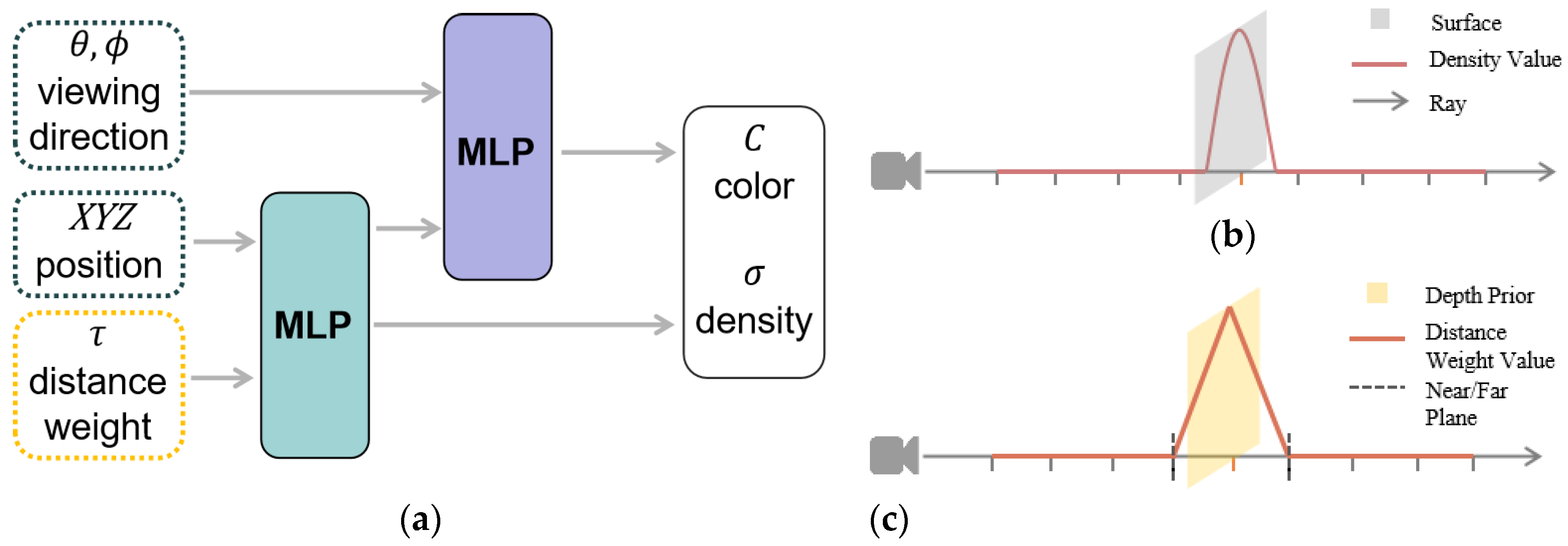
NeRF only accepts two inputs: location and viewing direction. The MLP uses location information to determine a consistent relationship between multiple views and to estimate the object’s surface, distance, and color. Simultaneously, the MLP uses the viewing direction information to present the light and shadow changes from different viewpoints. However, the NeRF sampling method has a different sampling rate in space. In densely sampled areas, NeRF produces remarkably realistic results. In less densely sampled areas, neither the depth nor the color values can be satisfactorily predicted. Particularly, the sampling density is further reduced after we guide the sampling through the depth prior, which causes the network model to not always fit as expected. To improve the predictive power of the network model at sparse sampling volume densities, we introduced distance weight information into the model to guide the model for training and prediction, as shown in Figure 3a. Network models fundamentally fail to render high-quality images because the volume density of sampling points on the ray is incorrectly estimated, and a good density distribution along the ray (Figure 3b) should satisfy the following conditions: (a) the density distribution is unimodal from the near plane to the object’s surface; (b) the volume density increases with increasing proximity to the object’s surface; and (c) the volume density of the area away from the object’s surface is close to zero. Although our dynamic sampling approach indirectly achieves the third requirement, estimation errors still exist. To drive the predicted density distribution to satisfy the first two requirements, we encoded depth priors as distance weights ${\tau }_i$. The weight score increases with the sampling point’s proximity to the prior depth. As shown in Figure 3c, the distance weight setting conforms to the characteristics of a good density distribution and can guide the MLP to predict volume density more accurately to obtain more accurate depth information.

$${\tau }_i=1-\frac{\left|S_i-D_p\right|}{\theta },$$

(6)

where $S_i$ denotes the sampling point and $D_p$ and $\theta$ denote the depth prior and controllable range constraint values, respectively. We guided the model to correct its depth predictions by including distance weight as a new dimension to the input vector.

4.3. Loss Function

We used a combined loss function that included RGB and depth loss functions to guide the training of the network using both RGB and depth information. Because our dynamic sampling and distance weighting methods already effectively guide the network for depth prediction, we design the depth loss as a simple mean squared loss.

$$L=L_c+\lambda L_d,$$

(7)

$$L_d={\displaystyle \sum _{r\in R}}{||\widehat{D}\left(r\right)-D\left(r\right)||}_2^2,\widehat{D}={\displaystyle \sum _{n=1}^N} {\omega }_n{t}_n,$$

(8)

where $L_c$ denotes the RGB loss, $L_d$ denotes the depth loss, $\lambda$ denotes the coefficient, $\widehat{D}$ denotes the estimated depth distance along the ray, and $t_n$ denotes the position of the sampling point on the ray.

4.4. Depth Prior Acquisition and Hybrid Rendering

Both the dynamic sampling and distance weighting methods are invalid because the prediction lacks depth priors. To address this problem, we obtained a depth map and an RBG image corresponding to the new viewpoint using the TMRM. First, we developed a truncated signed distance function (TSDF) [34] from the RGBD data in the training set, and constructed a TSDF-based 3D mesh using the marching cube algorithm [35]. Second, depth maps and RGB images of novel viewpoints were obtained quickly through the rendering pipeline. However, the training set data did not cover the entire scene, leaving a significant number of holes in both the depth map and RGB images.

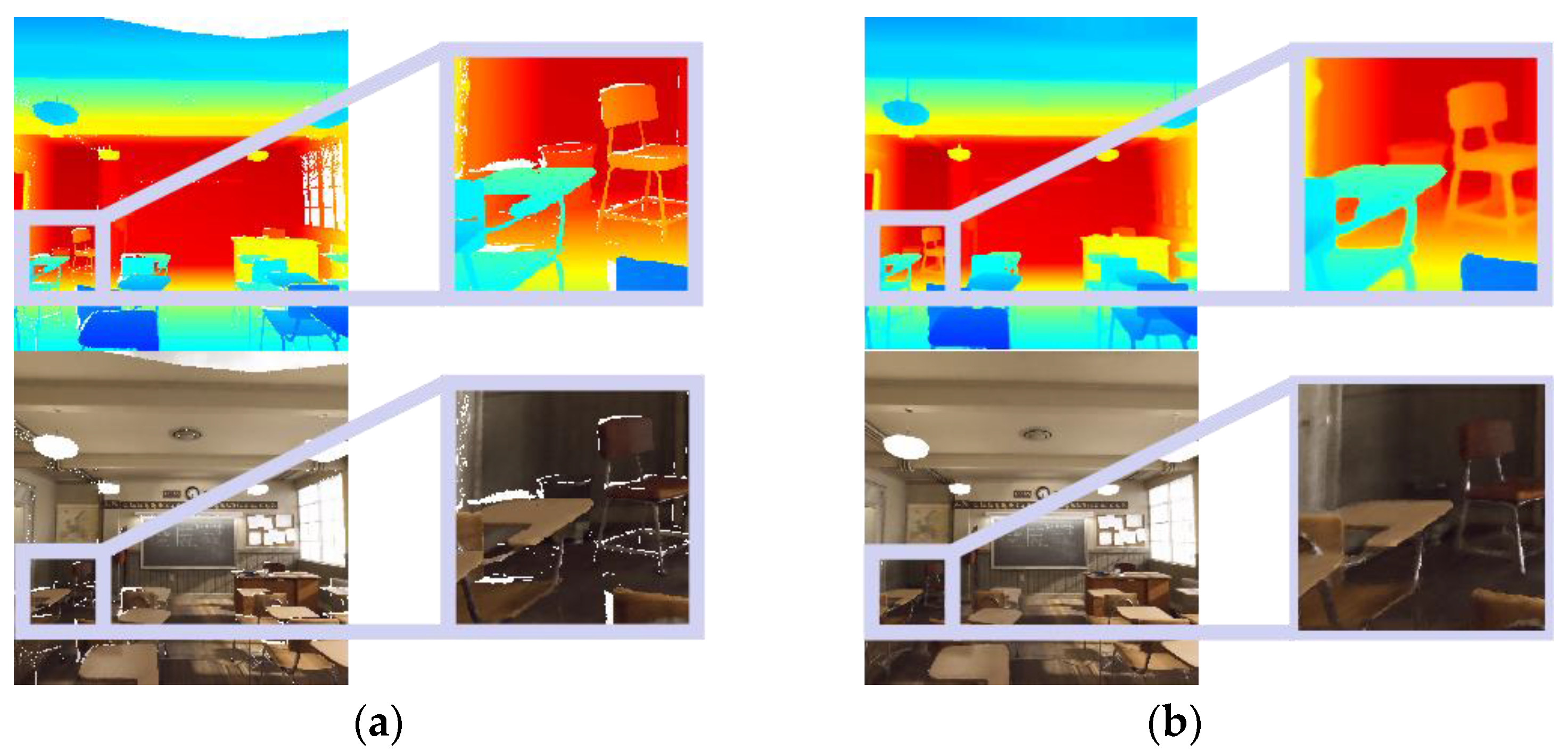
As shown in Figure 4a, the holes in the depth maps demonstrate the absence of depth priors, which prevents our NeRF model from rendering the entire result. For depth maps with holes, we used the traditional depth-completion algorithm IP-Basic [36] to perform the repair. As shown in Figure 4b, the completed depth map can guide the NeRF model to render the full image.

Although we reduced the number of sampling points using dynamic sampling, improved the rendering efficiency, and reduced the burden of hardware memory, we still require many sampling points for prediction calculation. Taking an 800 × 800 image as an example, even if each ray samples eight points, millions of sampling points must still be processed, which cannot meet the demand for fast rendering using the existing hardware. To accelerate rendering, we used RGB images obtained from the TMRM to synthesize novel views (Figure 5a). Because TMRM is significantly efficient at rendering, resulting in a good quality image in flat areas, we need only repair the hole areas of images using our NeRF model to obtain high-quality images (Figure 5b). Additionally, we used the weight smoothing method to address the color difference between NeRF and traditional mesh rendering and realized hybrid rendering through gradual weight distribution (Figure 5c).

The hybrid rendering method was used to further reduce the hardware overhead of the sampling points. For the rendering of each novel view, the demand for sampling points can be reduced by 60–90% on average.

5. Results

5.1. Dataset and Set

We validated the effectiveness of our method using a dataset collected by DONeRF, which exhibits both fine and high-frequency details, as well as large depth ranges. The dataset was rendered using Blender, and the poses were randomly sampled within a view cell. The 300 high-quality images and depth maps for each scene were divided into training (210), test (60), and validation (30) sets. To verify the effectiveness of our method with sparse inputs, we randomly selected 11 images from the original training set, while the test and validation sets were kept unchanged. In practice, we mainly used three scenes for our comparison experiments: Classroom, Barbershop, and San Miguel. Our NeRF model uses the Adam optimizer, with a learning rate of 5 × 10⁻⁴, an eight-layer network depth, a single-layer dimension of 256, and 200,000 iterations. To verify the robustness of our algorithm under sparse input conditions, we unified the number of sampling points into eight coarse and eight fine sampling points.

5.2. Evaluation Metrics

Peak signal-to-noise ratio (PSNR) is a widely used objective evaluation metric for images, which is based on the calculation of the error between the corresponding pixels.

Structural similarity (SSIM) is an evaluation metric for measuring the similarity of two images and it models distortion as a combination of brightness, contrast, and structure.

Learning to perceive image block similarity (LPIPS) is a deep learning-based image similarity evaluation metric, which extracts depth features for comparison through a neural network.

Time is described as the time consumed to render a single image and is set in seconds.

5.3. Comparisons

We compared our method with DONeRF, the current state-of-the-art algorithm for guiding NeRF model training and prediction using deep priors. We found that both models shared the core principles. Additionally, we compared our method with the TMRM to demonstrate the effectiveness of our hybrid rendering method.

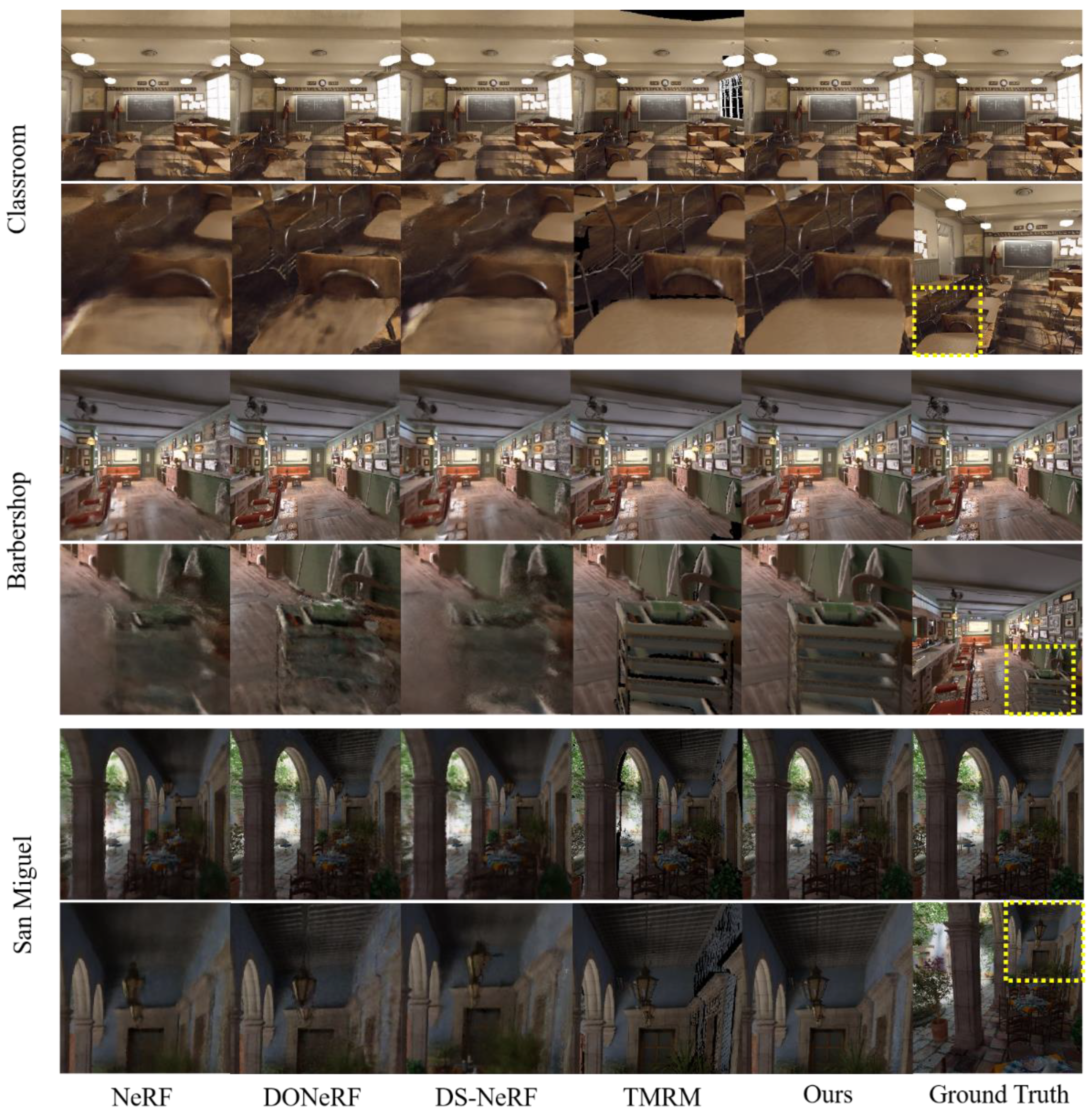
Figure 6 compares the prediction results of our method and other advanced methods, and the results demonstrate that our method outperforms the other methods in terms of visual observation. The original NeRF did not use additional priors to guide the model for training or prediction, resulting in severe blurring of novel views rendered with sparsely sampled points. DONeRF uses depth information to train a sampling Oracle network, which can help the model to determine the best sampling locations. However, with fewer input images, the prediction accuracy of the sampling Oracle network decreases, resulting in blurring of novel views. DS-NeRF focuses on a sparse set of input photos and enhances the generalization of the model by introducing depth loss. However, there is no significant improvement in the rendering quality of DS-NeRF compared to the original nerf for larger scenes. The TMRM only produces good results in partially flat depth areas, whereas there are many holes owing to blocking in other areas. Our method introduces a depth prior in the sampling method, input data, and a loss function to effectively guide the model to render high-quality images despite the reduced input images. Additionally, we combined our NeRF with the TMRM for hybrid rendering. The TMRM has faster rendering capabilities and achieves good rendering quality in depth-flat areas, whereas our NeRF complements the hole areas for efficient and high-quality rendering.

Table 1. Test results for different methods, and the bold values are the best.

	Classroom			Barbershop			San Miguel			Average
Method	SSIM↑	PSNR↑	LPIPS↓	SSIM↑	PSNR↑	LPIPS↓	SSIM↑	PSNR↑	LPIPS↓	SSIM↑	PSNR↑	LPIPS↓	Time(s)↓
NeRF (8 + 8)	0.78	24.42	0.25	0.74	23.03	0.29	0.59	22.13	0.40	0.70	23.19	0.31	5.7
DONeRF (8 + 8)	0.83	25.11	0.16	0.80	24.04	0.20	0.68	22.97	0.27	0.77	24.04	0.21	4.8
DS-NeRF (8 + 8)	0.77	24.27	0.26	0.74	23.29	0.28	0.59	22.05	0.42	0.70	23.20	0.32	5.3
TMRM	0.80	17.92	0.15	0.81	22.61	0.14	0.74	21.44	0.15	0.78	20.66	0.15	0.6
Ours (Hybrid)	0.86	25.88	0.10	0.85	25.15	0.12	0.77	24.15	0.13	0.83	25.06	0.12	0.6 + 1.2

compares the advantages of our method with those of other methods in terms of the evaluation metrics. Our approach differs from DONeRF in two ways. First, in the sampling method, we obtained depth priors using the TMRM and added dynamic sampling to the prediction. Second, we encoded the depth prior as the depth weights to participate in the model training and prediction. Based on these changes, the model aided in resolving blurring problems caused by sparse sampling. Additionally, the images obtained using the TMRM had the lowest PSNR scores because of the high number of holes, but obtained excellent SSIM and LPIPS scores, indicating that the TMRM can produce partially high-quality rendered areas. Particularly, the TMRM had the fastest rendering speed, which is needed for NeRF-based models. The hybrid rendering method repaired the holes that formed in the TMRM by combining the advantages of both methods for the best performance possible.

5.4. Ablation Study

Experiments were conducted on relevant datasets to verify the validity of Dynamic Sampling, Distance Weight, and Hybrid Rendering. According to

Table 2. Test results of the ablation study, and the bold values are the best.

	Classroom			Barbershop			San Miguel			Average
Method	SSIM↑	PSNR↑	LPIPS↓	SSIM↑	PSNR↑	LPIPS↓	SSIM↑	PSNR↑	LPIPS↓	SSIM↑	PSNR↑	LPIPS↓
Ours (w/o D.S., Hybrid)	0.75	23.85	0.28	0.72	22.84	0.29	0.51	20.52	0.47	0.66	22.40	0.35
Ours (w/o D.W., Hybrid)	0.81	25.23	0.18	0.80	24.89	0.20	0.67	23.26	0.29	0.76	24.46	0.22
Ours (w/o Hybrid)	0.83	25.78	0.16	0.80	24.95	0.18	0.68	23.32	0.27	0.77	24.68	0.20
Ours	0.86	25.88	0.10	0.85	25.15	0.12	0.77	24.15	0.13	0.83	25.06	0.12

, the method that introduces Dynamic Sampling and Distance Weight does perform, but Hybrid Rendering is the best in all metrics (SSIM, PSNR, and LPIPS).

Without Hybrid Rendering: The TMRM gives high quality rendering results in some areas of the image; adding Hybrid Rendering can improve rendering efficiency while improving rendering quality.

Without Dynamic Sampling and Hybrid Rendering: Removing the dynamic sampling method causes the distance between the sampled points to grow, and the error of the distance weights increases with the distance in regions where the depth prior is uncertain. This affects the normal convergence of the model causing blurry predicted images.

Without Distance Weight and Hybrid Rendering: Removing the distance weighting method decreases the score for each evaluation metric. This is because the NeRF model, which lacks distance weights, still suffers from underfitting in sparsely sampled regions of space. Adding the distance weights can help NeRF address this problem. As shown in Figure 7, the rendered image is blurry in the area close to the viewpoint because of the low density of the sampled points, which becomes evident after the introduction of distance weights.

6. Limitations

Our approach allows the use of sparse images as input in the novel view synthesis task for large scenes while maintaining rendering quality and efficiency. However, because our approach relies on depth priors, an incorrect depth prior can reduce rendering quality. When the input view is more sparse, depth maps obtained using the TMRM have a larger area of holes, making it difficult for traditional depth-completion methods to accurately complete the depth maps, which reduces the prediction accuracy of our NeRF model. Future work can further refine the depth-completion method to improve the robustness of the NeRF model in the presence of missing depth priors.

7. Conclusions

We propose a novel view-synthesis method based on NeRF. Unlike previous methods that used a depth prior, we used dynamic sampling and distance weights to help the model make predictions by acting on the depth prior as far in advance as possible of the model input. Compared with the method of training the model with a depth loss function, our method achieved higher quality rendering with a sparser input view and fewer sampling points. Additionally, we exploited the efficiency of the TMRM to accelerate the rendering of our NeRF-based model while maintaining the rendering quality. Overall, we have developed a novel view synthesis method to help novel view-rendering methods improve both rendering quality and efficiency.

References

1. Mildenhall, B.; Srinivasan, P.P.; Tancik, M.; Barron, J.T.; Ramamoorthi, R.; Ng, R. Nerf: Representing scenes as neural radiance fields for view synthesis. Commun. ACM 2021, 65, 99–106. [Google Scholar] [CrossRef]
2. Barron, J.T.; Mildenhall, B.; Tancik, M.; Hedman, P.; Martin-Brualla, R.; Srinivasan, P.P. Mip-nerf: A multiscale representation for anti-aliasing neural radiance fields. In Proceedings of the IEEE/CVF International Conference on Computer Vision 2021, Montreal, BC, Canada, 10–17 October 2021; pp. 5855–5864. [Google Scholar]
3. Tancik, M.; Casser, V.; Yan, X.; Pradhan, S.; Mildenhall, B.; Srinivasan, P.P.; Barron, J.T.; Kretzschmar, H. Block-nerf: Scalable large scene neural view synthesis. In Proceedings of the IEEE/CVF Conference on Computer Vision and Pattern Recognition 2022, New Orleans, LA, USA, 19–24 June 2022; pp. 8248–8258. [Google Scholar]
4. Martin-Brualla, R.; Radwan, N.; Sajjadi, M.S.; Barron, J.T.; Dosovitskiy, A.; Duckworth, D. Nerf in the wild: Neural radiance fields for unconstrained photo collections. In Proceedings of the IEEE/CVF Conference on Computer Vision and Pattern Recognition 2021, Nashville, TN, USA, 20–25 June 2020; pp. 7210–7219. [Google Scholar]
5. Kajiya, J.T.; Von Herzen, B.P. Ray tracing volume densities. ACM SIGGRAPH Comput. Graph. 1984, 18, 165–174. [Google Scholar] [CrossRef]
6. Zhang, X.; Srinivasan, P.P.; Deng, B.; Debevec, P.; Freeman, W.T.; Barron, J.T. Nerfactor: Neural factorization of shape and reflectance under an unknown illumination. ACM Trans. Graph. (TOG) 2021, 40, 1–18. [Google Scholar] [CrossRef]
7. Deng, K.; Liu, A.; Zhu, J.Y.; Ramanan, D. Depth-supervised nerf: Fewer views and faster training for free. In Proceedings of the IEEE/CVF Conference on Computer Vision and Pattern Recognition 2022, New Orleans, LA, USA, 19–24 June 2022; pp. 12882–12891. [Google Scholar]
8. Karnewar, A.; Ritschel, T.; Wang, O.; Mitra, N. Relu fields: The little non-linearity that could. In ACM SIGGRAPH 2022 Conference Proceedings; Association for Computing Machinery: New York, NY, USA, 2022; pp. 1–9. [Google Scholar]
9. Garbin, S.J.; Kowalski, M.; Johnson, M.; Shotton, J.; Valentin, J. Fastnerf: High-fidelity neural rendering at 200fps. In Proceedings of the IEEE/CVF International Conference on Computer Vision 2021, Montreal, BC, Canada, 10–17 October 2021; pp. 14346–14355. [Google Scholar]
10. Yuan, Y.J.; Lai, Y.K.; Huang, Y.H.; Kobbelt, L.; Gao, L. Neural radiance fields from sparse RGB-D images for high-quality view synthesis. In IEEE Transactions on Pattern Analysis and Machine Intelligence; IEEE: New York, NY, USA, 2022. [Google Scholar]
11. Wei, Y.; Liu, S.; Rao, Y.; Zhao, W.; Lu, J.; Zhou, J. Nerfingmvs: Guided optimization of neural radiance fields for indoor multi-view stereo. In Proceedings of the IEEE/CVF International Conference on Computer Vision 2021, Montreal, BC, Canada, 10–17 October 2021; pp. 5610–5619. [Google Scholar]
12. Rematas, K.; Liu, A.; Srinivasan, P.P.; Barron, J.T.; Tagliasacchi, A.; Funkhouser, T.; Ferrari, V. Urban radiance fields. In Proceedings of the IEEE/CVF Conference on Computer Vision and Pattern Recognition 2022, New Orleans, LA, USA, 19–24 June 2022; pp. 12932–12942. [Google Scholar]
13. Roessle, B.; Barron, J.T.; Mildenhall, B.; Srinivasan, P.P.; Nießner, M. Dense depth priors for neural radiance fields from sparse input views. In Proceedings of the IEEE/CVF Conference on Computer Vision and Pattern Recognition 2022, New Orleans, LA, USA, 19–24 June 2022; pp. 12892–12901. [Google Scholar]
14. Neff, T.; Stadlbauer, P.; Parger, M.; Kurz, A.; Mueller, J.H.; Chaitanya, C.R.; Kaplanyan, A.A.; Steinberger, M. DONeRF: Towards Real-Time Rendering of Compact Neural Radiance Fields using Depth Oracle Networks. Comput. Graph. Forum 2021, 40, 45–59. [Google Scholar] [CrossRef]
15. Murez, Z.; Van As, T.; Bartolozzi, J.; Sinha, A.; Badrinarayanan, V.; Rabinovich, A. Atlas: End-to-end 3d scene reconstruction from posed images. In Proceedings of the European Conference on Computer Vision 2020, Online, 23–28 August 2020; pp. 414–431. [Google Scholar]
16. Curless, B.; Levoy, M. A volumetric method for building complex models from range images. In Proceedings of the 23rd Annual Conference on Computer Graphics and Interactive Techniques 1996, New Orleans, LA, USA, 4–9 August 1996; pp. 303–312. [Google Scholar]
17. Dai, A.; Nießner, M.; Zollhöfer, M.; Izadi, S.; Theobalt, C. Bundlefusion: Real-time globally consistent 3d reconstruction using on-the-fly surface reintegration. ACM Trans. Graph. 2017, 36, 1. [Google Scholar] [CrossRef]
18. Izadi, S.; Kim, D.; Hilliges, O.; Molyneaux, D.; Newcombe, R.; Kohli, P.; Shotton, J.; Hodges, S.; Freeman, D.; Davison, A.; et al. KinectFusion: Real-time 3D reconstruction and interaction using a moving depth camera. In Proceedings of the 24th Annual ACM Symposium on User Interface Software and Technology 2011, Santa Barbara, CA, USA, 16–19 October 2011; pp. 559–568. [Google Scholar]
19. Nießner, M.; Zollhöfer, M.; Izadi, S.; Stamminger, M. Real-time 3D reconstruction at scale using voxel hashing. ACM Trans. Graph. 2013, 32, 1–11. [Google Scholar] [CrossRef] [Green Version]
20. Kazhdan, M.; Bolitho, M.; Hoppe, H. Poisson surface reconstruction. In Proceedings of the Fourth Eurographics Symposium on Geometry processing 2006, Cagliari Sardinia, Italy, 26–28 June 2006. [Google Scholar]
21. Pfister, H.; Zwicker, M.; Van Baar, J.; Gross, M. Surfels: Surface elements as rendering primitives. In Proceedings of the 27th Annual Conference On Computer Graphics And Interactive Techniques 2000, New Orleans, LA, USA, 23–28 July 2000; pp. 335–342. [Google Scholar]
22. Marton, Z.C.; Rusu, R.B.; Beetz, M. On fast surface reconstruction methods for large and noisy point clouds. In Proceedings of the 2009 IEEE International Conference on Robotics and Automation 2009, Kobe, Japan, 12–17 May 2009; pp. 3218–3223. [Google Scholar]
23. Yu, A.; Ye, V.; Tancik, M.; Kanazawa, A. pixelnerf: Neural radiance fields from one or few images. In Proceedings of the IEEE/CVF Conference on Computer Vision and Pattern Recognition 2021, Nashville, TN, USA, 20–25 June 2020; pp. 4578–4587. [Google Scholar]
24. Tancik, M.; Mildenhall, B.; Wang, T.; Schmidt, D.; Srinivasan, P.P.; Barron, J.T.; Ng, R. Learned initializations for optimizing coordinate-based neural representations. In Proceedings of the IEEE/CVF Conference on Computer Vision and Pattern Recognition 2021, Nashville, TN, USA, 20–25 June 2020; pp. 2846–2855. [Google Scholar]
25. Turki, H.; Ramanan, D.; Satyanarayanan, M. Mega-NeRF: Scalable Construction of Large-Scale NeRFs for Virtual Fly-Throughs. In Proceedings of the IEEE/CVF Conference on Computer Vision and Pattern Recognition 2022, New Orleans, LA, USA, 19–24 June 2022; pp. 12922–12931. [Google Scholar]
26. Zhang, K.; Riegler, G.; Snavely, N.; Koltun, V. Nerf++: Analyzing and improving neural radiance fields. arXiv 2020, arXiv:2010.07492. [Google Scholar]
27. Lin, C.H.; Ma, W.C.; Torralba, A.; Lucey, S. Barf: Bundle-adjusting neural radiance fields. In Proceedings of the IEEE/CVF International Conference on Computer Vision 2021, Montreal, BC, Canada, 10–17 October 2021; pp. 5741–5751. [Google Scholar]
28. Meng, Q.; Chen, A.; Luo, H.; Wu, M.; Su, H.; Xu, L.; He, X.; Yu, J. Gnerf: Gan-based neural radiance field without posed camera. In Proceedings of the IEEE/CVF International Conference on Computer Vision 2021, Montreal, BC, Canada, 10–17 October 2021; pp. 6351–6361. [Google Scholar]
29. Goodfellow, I.; Pouget-Abadie, J.; Mirza, M.; Xu, B.; Warde-Farley, D.; Ozair, S.; Courville, A.; Bengio, Y. Generative adversarial networks. Commun. ACM 2020, 63, 139–144. [Google Scholar] [CrossRef]
30. Yu, A.; Li, R.; Tancik, M.; Li, H.; Ng, R.; Kanazawa, A. Plenoctrees for real-time rendering of neural radiance fields. In Proceedings of the IEEE/CVF International Conference on Computer Vision 2021, Montreal, BC, Canada, 10–17 October 2021; pp. 5752–5761. [Google Scholar]
31. Liu, L.; Gu, J.; Zaw Lin, K.; Chua, T.S.; Theobalt, C. Neural sparse voxel fields. Adv. Neural Inf. Process. Syst. 2020, 33, 15651–15663. [Google Scholar]
32. Müller, T.; Evans, A.; Schied, C.; Keller, A. Instant neural graphics primitives with a multiresolution hash encoding. arXiv 2022, arXiv:2201.05989. [Google Scholar]
33. Vaswani, A.; Shazeer, N.; Parmar, N.; Uszkoreit, J.; Jones, L.; Gomez, A.N.; Kaiser, Ł.; Polosukhin, I. Attention is all you need. In Proceedings of the Advances in Neural Information Processing systems, Long Beach, CA, USA, 4–9 December 2017; pp. 5998–6008. [Google Scholar]
34. Werner, D.; Al-Hamadi, A.; Werner, P. Truncated signed distance function: Experiments on voxel size. In Proceedings of the International Conference Image Analysis and Recognition 2014, Vilamoura, Portugal, 22–24 October 2014; pp. 357–364. [Google Scholar]
35. Lorensen, W.E.; Cline, H.E. Marching cubes: A high resolution 3D surface construction algorithm. ACM Siggraph Comput. Graph. 1987, 21, 163–169. [Google Scholar] [CrossRef]
36. Ku, J.; Harakeh, A.; Waslander, S.L. In defense of classical image processing: Fast depth completion on the cpu. In Proceedings of the 2018 15th Conference on Computer and Robot Vision, Toronto, ON, Canada, 8–10 May 2018; pp. 16–22. [Google Scholar]
Figure 1. The overall framework of the proposed method includes two parts: training and prediction. The provided depth information is used as priors for training, while the depth information obtained from traditional mesh rendering is used as priors for prediction. Finally, the neural radiation field (NeRF) model is used to fix holes in the images obtained by the traditional mesh rendering method (TMRM).
Electronics 12 01014 g001
Figure 2. (a) Original NeRF sampling method with no depth priors for wide range sampling; (b) Dynamic sampling approach, which removes several sampling points away from the surface of the object and only acquires sampling points near the surface of the object.
Electronics 12 01014 g002
Figure 3. (a) Depth prior encoded as distance weights and used as additional input to the first MLP; (b) A good density distribution only produces values greater than 0 near the surface of the object; (c) The distribution of the generated distance weights is close to a good density distribution.
Electronics 12 01014 g003
Figure 4. The effect of missing depth priors on the rendering of NeRF models: (a) A depth map with holes cannot guide our NeRF model to render a complete image; (b) Completed depth map can guide our NeRF model to render a complete image.
Electronics 12 01014 g004
Figure 5. (a) Holes in images obtained by the TMRM; (b) For areas with holes, our NeRF model was used for repair; (c) RGB values are determined during hybrid rendering based on the weights, with smaller weights preferring the values rendered by NeRF and larger weights preferring the values rendered by TMRM.
Electronics 12 01014 g005
Figure 6. Comparison of results between our method and other advanced methods. Each scene has a panorama and a partial view for comparison. Additionally, our method shows the best results for both panoramas and partial views.
Electronics 12 01014 g006
Figure 7. (a) The rendering result of our method (without distance weights) produces blurring in near viewpoint areas; (b) Distance weights can remove blurring.
Electronics 12 01014 g007