
A Fast Power Lines RCS Calculation Method Combining IEDG with CM-SMWA

Abstract
:1. Introduction
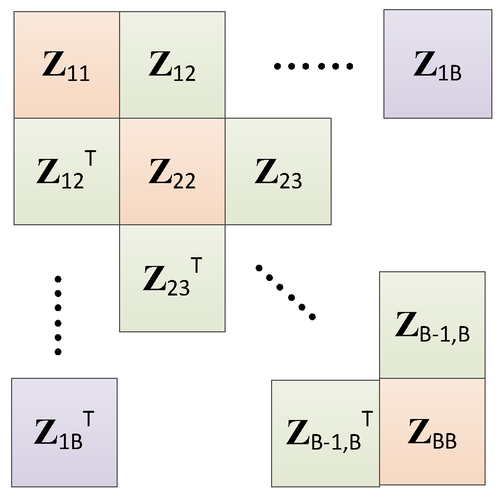
2. CM-SMWA
3. RCS Calculation Method of Power Line Combining IEDG and CM-SMWA
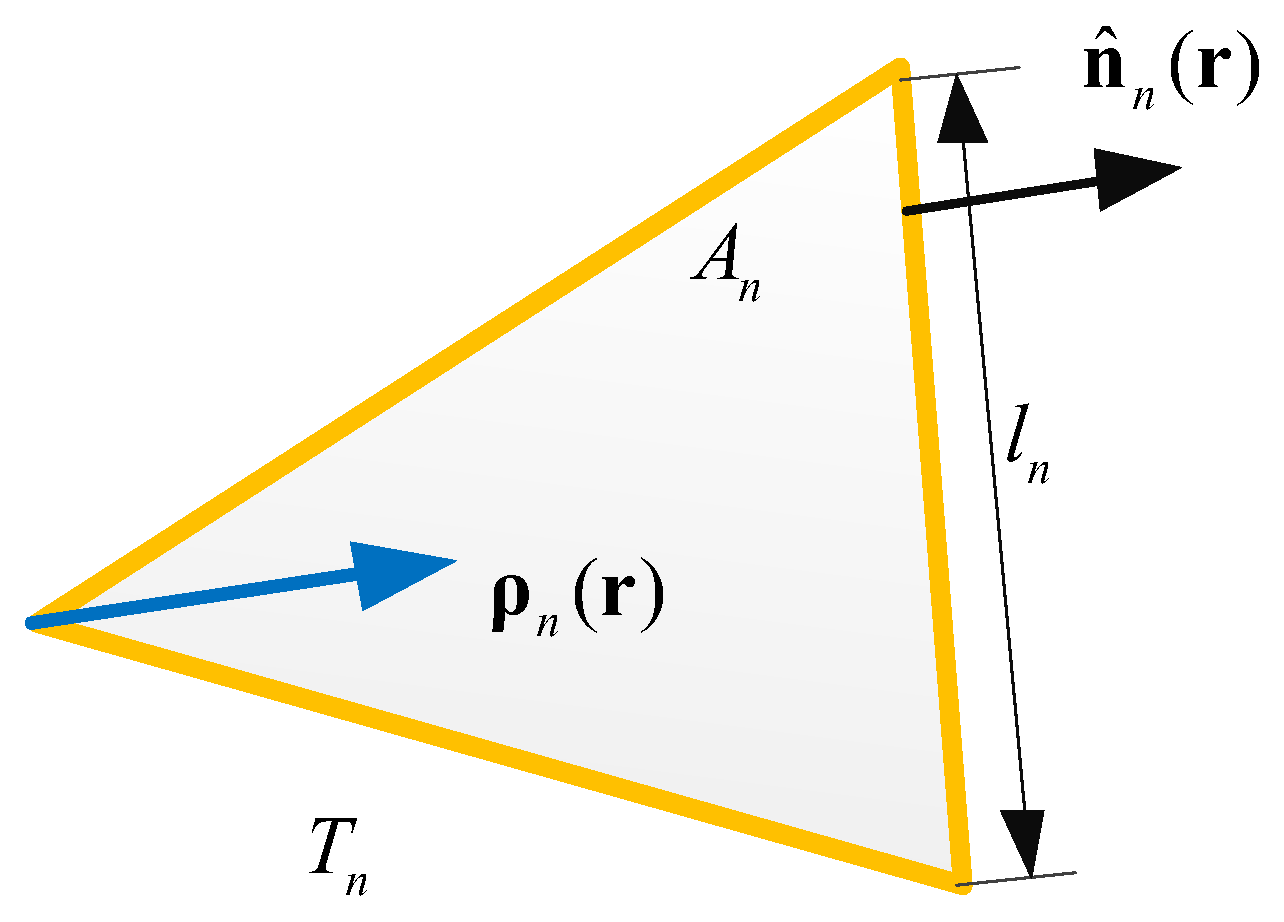
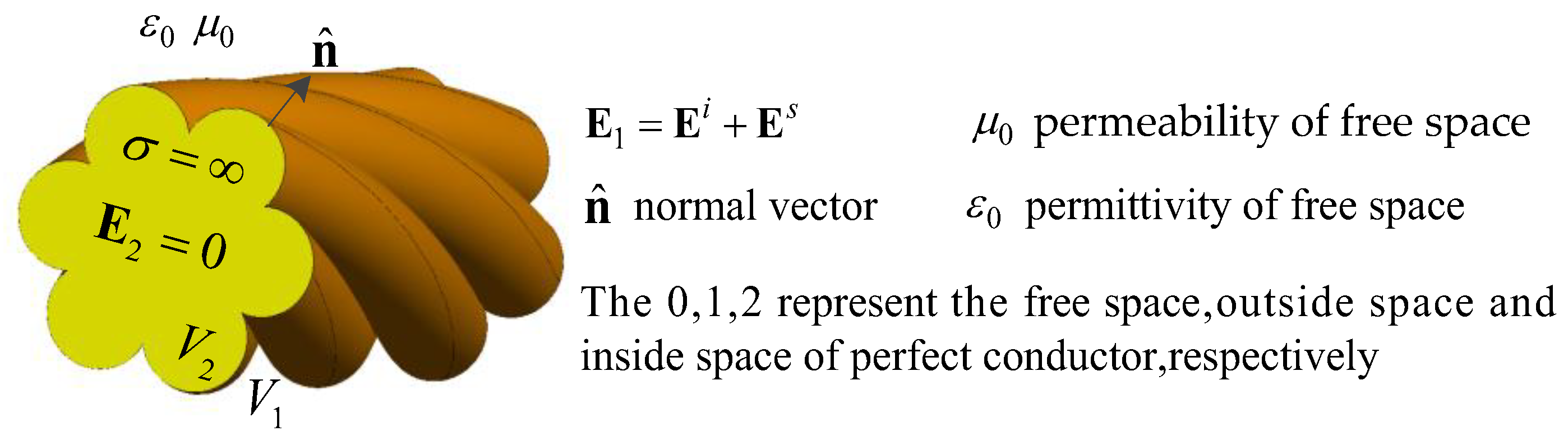
3.1. IEDG
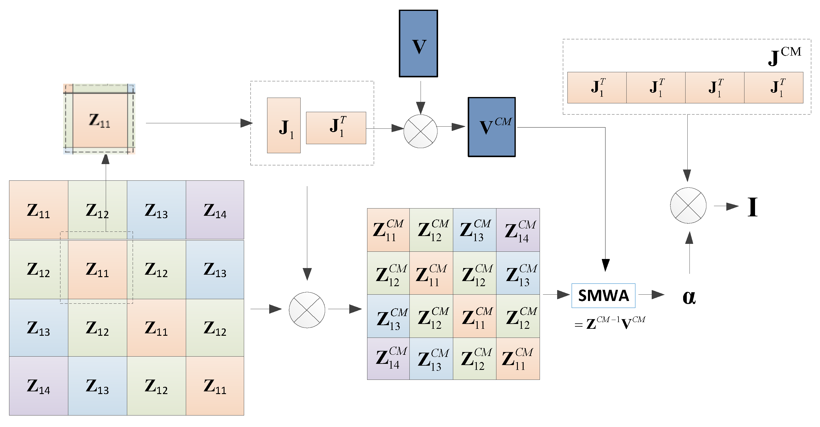
3.2. Power Line RCS Calculation by IEDG with CM-SMWA
4. Experimental Results and Analysis
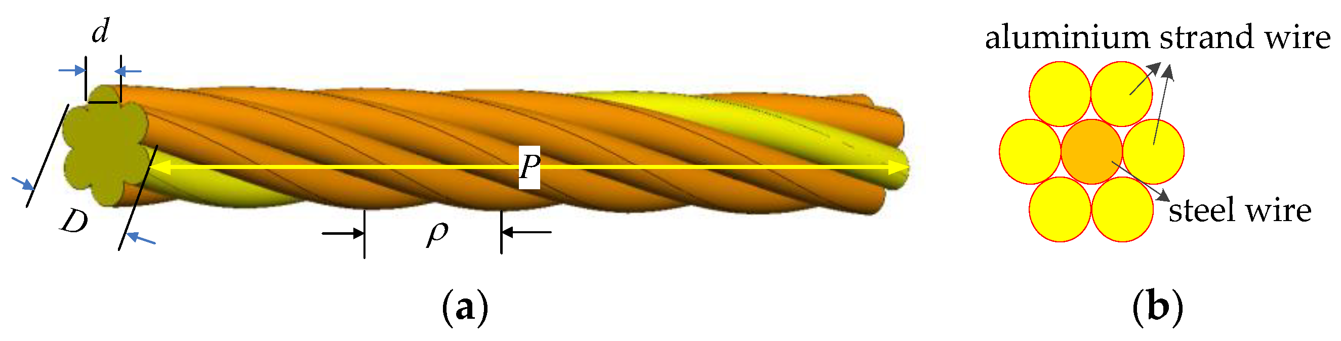
4.1. Simulated Models
4.2. Evaluation Indicators
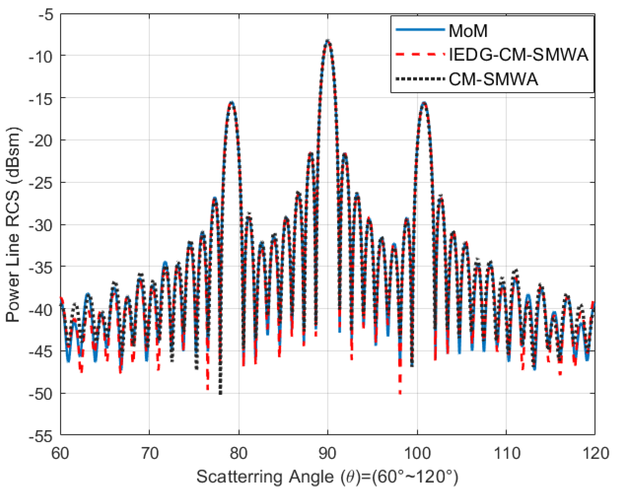
4.3. Numerical Calculation Comparison
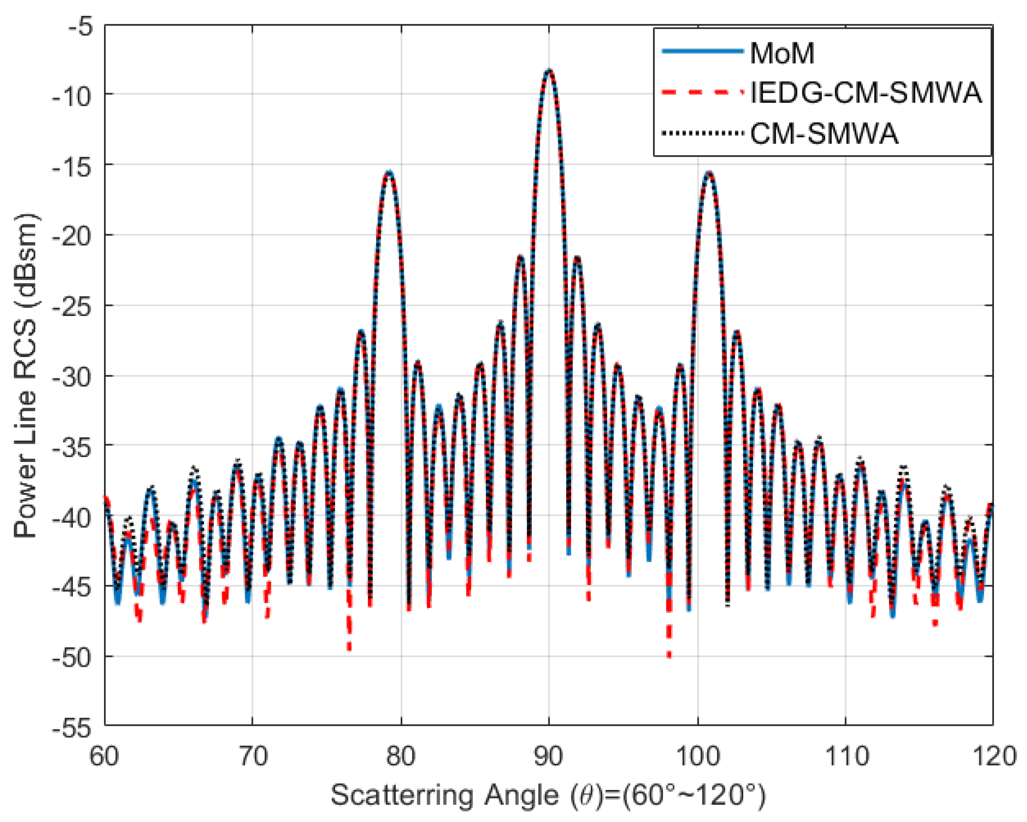
- (1)
- Simulation of incident wave frequency at 35 GHz
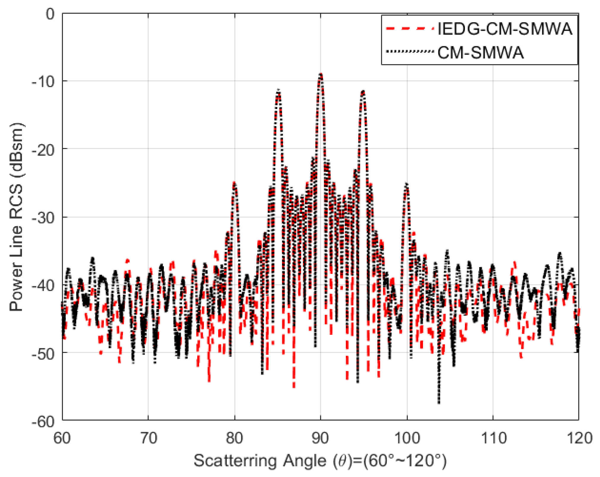
- (2)
- Simulation of incident wave frequency at 76 GHz
5. Conclusions
Author Contributions
Funding
Institutional Review Board Statement
Informed Consent Statement
Data Availability Statement
Conflicts of Interest
References
- Chandrasekaran, R.; Payan, A.P.; Collins, K.B. Helicopter Wire Strike Protection and Prevention Devices: Review, Challenges, And Recommendations. Aerosp. Sci. Technol. 2020, 98, 105665. [Google Scholar] [CrossRef]
- Rao, A.H.; Marais, K. High Risk Occurrence Chains in Helicopter Accidents. Reliab. Eng. Syst. Saf. 2018, 170, 83–98. [Google Scholar] [CrossRef]
- Goshi, D.S.; Case, T.J.; Mckitterick, J.B.; Long, Q.B. Multifunctional Millimeter Wave Radar System for Helicopter Safety. Proc. SPIE—Int. Soc. Opt. Eng. 2012, 8361, 173. [Google Scholar]
- Kumar, B.A.; Ghose, D. Radar-Assisted Collision Avoidance/Guidance Strategy for Planar Flight. IEEE Trans. Aerosp. Electron. Syst. 2001, 37, 77–90. [Google Scholar] [CrossRef]
- Goshi, D.S.; Mai, K.; Liu, Y.; Bui, L. A Millimeter-Wave Sensor Development System for Small Airborne Platforms. In Proceedings of the IEEE National Radar Conference Proceedings, Atlanta, GA, USA, 7–11 May 2012; pp. 510–515. [Google Scholar]
- Migliaccio, C.; Nguyen, B.D.; Pichot, C.; Yonemoto, N.; Yamamoto, K.; Yamada, K.; Nasui, H.; Mayer, W.; Gronau, A.; Menzel, W. Millimeter-Wave Radar for Rescue Helicopters. In Proceedings of the International Conference on Control, Kaunas, Lithuania, 4–5 May 2006; pp. 1–6. [Google Scholar]
- Al-Khatib, H.H. Laser and Millimeter-Wave Backscatter of Transmission Cables. In Proceedings of the Technical Symposium, Washington, DC, USA, 13–15 October 1982. [Google Scholar]
- Sarabandi, K.; Park, M. Millimeter-Wave Radar Phenomenology of Power Lines and a Polarimetric Detection Algorithm. IEEE Trans. Antennas Propag. 1999, 47, 1807–1813. [Google Scholar] [CrossRef]
- Sarabandi, K.; Park, M. Extraction of Power Line Maps from Millimeter-Wave Polarimetric SAR Images. IEEE Trans. Antennas Propag. 2000, 48, 1802–1809. [Google Scholar] [CrossRef]
- Xiong, W.; Luo, J.; Yu, C. Power Line Detection in Millimeter-Wave Radar Images Applying Convolutional Neural Networks. IET Radar Sonar Navig. 2021, 15, 1083–1095. [Google Scholar] [CrossRef]
- Qirong, M.; Darren, S.G.; Yi-Chi, S.; Ming-Ting, S. An Algorithm for Power Line Detection and Warning Based on a Millimeter-Wave Radar Video. IEEE Trans. Image Process. 2011, 20, 3534–3543. [Google Scholar] [CrossRef] [PubMed]
- Sarabandi, K.; Park, M. A Radar Cross-Section Model for Power Lines at Millimeter-Wave Frequencies. IEEE Trans. Antennas Propag. 2003, 51, 2353–2360. [Google Scholar] [CrossRef]
- Gibson, W.C. The Method of Moments in Electromagnetics; Taylor & Francis: New York, NY, USA, 2021. [Google Scholar]
- Chew, W.C.; Michielssen, E.; Song, J.M.; Jin, J.-M. Fast and Efficient Algorithms in Computational Electromagnetics; Artech House, Inc.: Norwood, MA, USA, 2001. [Google Scholar]
- Kalfa, M.; Ergül, Ö.; Ertürk, V.B. Error Control of Multiple-Precision MLFMA. IEEE Trans. Antennas Propag. 2018, 66, 5651–5656. [Google Scholar] [CrossRef]
- Sharma, S.; Triverio, P. AIMx: An Extended Adaptive Integral Method for the Fast Electromagnetic Modeling of Complex Structures. IEEE Trans. Antennas Propag. 2021, 69, 8603–8617. [Google Scholar] [CrossRef]
- Seo, S.M. A Fast IE-FFT Algorithm to Analyze Electrically Large Planar Microstrip Antenna Arrays. IEEE Antennas Wirel. Propag. Lett. 2018, 17, 983–987. [Google Scholar] [CrossRef]
- Zhao, K.; Vouvakis, M.N.; Lee, J.-F. The Adaptive Cross Approximation Algorithm for Accelerated Method of Moments Computations of EMC. IEEE Trans. Electromagn. Compat. 2005, 47, 763–773. [Google Scholar] [CrossRef]
- Chen, C.; Yang, F.; Hu, C.; Zhou, J. An Improved RCS Calculation Method for Power Lines Combining Characteristic Mode with SMWA. Electronics 2022, 11, 2051. [Google Scholar] [CrossRef]
- Peng, Z.; Lim, K.; Lee, J. A Discontinuous Galerkin Surface Integral Equation Method for Electromagnetic Wave Scattering From Nonpenetrable Targets. IEEE Antennas Propag. Mag. 2013, 61, 3617–3628. [Google Scholar] [CrossRef]
- Zhang, L.; Sheng, X. A Discontinuous Galerkin Volume Integral Equation Method for Scattering from Inhomogeneous Objects. IEEE Trans. Antennas Propag. 2015, 63, 5661–5667. [Google Scholar] [CrossRef]
- Rao, S.; Wilton, D.; Glisson, A. Electromagnetic Scattering by Surfaces of Arbitrary Shape. IEEE Trans. Antennas Propag. 1982, 30, 409–418. [Google Scholar] [CrossRef]
- Angiulli, G.; Amendola, G.; Di Massa, G. Application of Characteristic Modes to the Analysis of Scattering from Microstrip Antennas. J. Electromagn. Waves Appl. 2000, 14, 1063–1081. [Google Scholar] [CrossRef]
- Guan, L.; He, Z.; Ding, D.; Chen, R. Efficient Characteristic Mode Analysis for Radiation Problems of Antenna Arrays. IEEE Trans. Antennas Propag. 2019, 67, 199–206. [Google Scholar] [CrossRef]
- Chen, X.; Gu, C.; Zhuo, L.; Niu, Z. Accelerated Direct Solution of Electromagnetic Scattering via Characteristic Basis Function Method With Sherman-Morrison-Woodbury Formula-Based Algorithm. IEEE Trans. Antennas Propag. 2016, 64, 4482–4486. [Google Scholar] [CrossRef]
- Fang, X.; Cao, Q.; Zhou, Y.; Yi, W. Multiscale Compressed and Spliced Sherman–Morrison–Woodbury Algorithm With Characteristic Basis Function Method. IEEE Trans. Electromagn. Compat. 2017, 60, 716–724. [Google Scholar] [CrossRef]
- Wang, K.; Li, M.; Ding, D.; Chen, R. A Parallelizable Direct Solution of Integral Equation Methods for Electromagnetic Analysis. Eng. Anal. Bound. Elem. 2017, 85, 158–164. [Google Scholar] [CrossRef]
- Rong, Z.; Jiang, M.; Chen, Y.; Lei, L.; Li, X.; Nie, Z.; Hu, J. Fast Direct Solution of Integral Equations with Modified HODLR Structure for Analyzing Electromagnetic Scattering Problems. IEEE Trans. Antennas Propag. 2019, 67, 3288–3296. [Google Scholar] [CrossRef]
- Ubeda, E.; Rius, J.M. Novel Monopolar MFIE MoM-Discretization for the Scattering Analysis of Small Objects. IEEE Trans. Antennas Propag. 2006, 54, 50–57. [Google Scholar] [CrossRef]
- Ziegler, V.; Schubert, F.; Schulte, B.; Giere, A.; Koerber, R. Helicopter Near-Field Obstacle Warning System Based on Low-Cost Millimeter-Wave Radar Technology. IEEE Trans. Microw. Theory Tech. 2013, 61, 658–665. [Google Scholar] [CrossRef]
- Kohmura, A.; Yonemoto, N.; Futatsumori, S.; Morioka, K. Evaluation of Polarisation Characteristics of Power-Line RCS at 76 GHz for Helicopter Obstacle Detection. Electron. Lett. 2015, 51, 1110–1111. [Google Scholar]


| Cases | m | n | Summation Terms |
|---|---|---|---|
| 1 | RWG | RWG | 1 |
| 2 | RWG | half-RWG | 1, 2 |
| 3 | half-RWG | RWG | 1, 3 |
| 4 | half-RWG | half-RWG | 1, 2, 3, 4 |
| Model | Steel Core | Outer Aluminum Strand/d | Diameter D | P | ρ |
|---|---|---|---|---|---|
| LGJ50-8 | 1 | 6/3.2 mm | 9.55 mm | 138 mm | 23 mm |
| Methods | Total Time | Relative Error |
|---|---|---|
| MoM | 7.3 min | -- |
| CM-SMWA | 6.3 min | 1.2% |
| IEDG-CM-SMWA | 1.9 min | 1.2% |
| Methods | Total Time | Relative Error |
|---|---|---|
| MoM | 7.3 min | -- |
| CM-SMWA | 4.2 min | 4.3% |
| IEDG-CM-SMWA | 1.9 min | 1.2% |
| Methods | Total Time | Relative Error |
|---|---|---|
| CM-SMWA | 56.3 min | |
| IEDG-CM-SMWA | 28.1 min | 2.8% |
| Methods | Total Time | Relative Error |
|---|---|---|
| CM-SMWA | 57.9 min | |
| IEDG-CM-SMWA | 26.4 min | 3.1% |
Disclaimer/Publisher’s Note: The statements, opinions and data contained in all publications are solely those of the individual author(s) and contributor(s) and not of MDPI and/or the editor(s). MDPI and/or the editor(s) disclaim responsibility for any injury to people or property resulting from any ideas, methods, instructions or products referred to in the content. |
© 2023 by the authors. Licensee MDPI, Basel, Switzerland. This article is an open access article distributed under the terms and conditions of the Creative Commons Attribution (CC BY) license (https://creativecommons.org/licenses/by/4.0/).
Share and Cite
Chen, C.; Hu, C.; Zhou, J. A Fast Power Lines RCS Calculation Method Combining IEDG with CM-SMWA. Electronics 2023, 12, 757. https://doi.org/10.3390/electronics12030757
Chen C, Hu C, Zhou J. A Fast Power Lines RCS Calculation Method Combining IEDG with CM-SMWA. Electronics. 2023; 12(3):757. https://doi.org/10.3390/electronics12030757
Chicago/Turabian StyleChen, Chunfeng, Changyu Hu, and Jianjiang Zhou. 2023. "A Fast Power Lines RCS Calculation Method Combining IEDG with CM-SMWA" Electronics 12, no. 3: 757. https://doi.org/10.3390/electronics12030757
APA StyleChen, C., Hu, C., & Zhou, J. (2023). A Fast Power Lines RCS Calculation Method Combining IEDG with CM-SMWA. Electronics, 12(3), 757. https://doi.org/10.3390/electronics12030757