3D Point Cloud Stitching for Object Detection with Wide FoV Using Roadside LiDAR

Abstract

Light Detection and Ranging (LiDAR) is widely used in the perception of physical environment to complete object detection and tracking tasks. The current methods and datasets are mainly developed for autonomous vehicles, which could not be directly used for roadside perception. This paper presents a 3D point cloud stitching method for object detection with wide horizontal field of view (FoV) using roadside LiDAR. Firstly, the base detection model is trained by KITTI dataset and has achieved detection accuracy of 88.94. Then, a new detection range of 180° can be inferred to break the limitation of camera’s FoV. Finally, multiple sets of detection results from a single LiDAR are stitched to build a 360° detection range and solve the problem of overlapping objects. The effectiveness of the proposed approach has been evaluated using KITTI dataset and collected point clouds. The experimental results show that the point cloud stitching method offers a cost-effective solution to achieve a larger FoV, and the number of output objects has increased by 77.15% more than the base model, which improves the detection performance of roadside LiDAR.

1. Introduction

Three-dimensional (3D) data play an important role in autonomous driving, domestic robots, and remote sensing [1,2]. Multiple data types such as point clouds, depth images, and polygon meshes are included in 3D data [3]. As a commonly used format, point clouds are generated by LiDAR, which has the capability to provide more accurate and valuable spatial information at 360°. LiDAR is insensitive to different light conditions and can perform stable work even under weak light environments [4,5,6].

Recently, point clouds have received much attention [7], and several studies of onboard LiDAR for 3D object detection have been proposed. The 3D object detection aims to perceive the location, size, and class of surrounding objects, and draw a bounding box to provide descriptions of shape and heading angle [8,9]. With the development of deep learning technology, existing approaches have been applied to autonomous vehicles to get accurate information and make effective predictions [10]. To build a real-time cooperative system, LiDAR has a new application that was installed on roadside infrastructures to obtain long-term trajectory data of all road users and serve autonomous vehicles [11,12,13]. Each road user can be scanned and shared with traffic facilities and autonomous vehicles by roadside LiDAR, which provides a solution to fill the data gap for intelligent transportation systems (ITS) [14,15].

However, such corresponding deep learning algorithms rely increasingly on benchmark datasets that are crucial for model training and evaluation [16]. In the case of LiDAR, although 360° scanning technology is used for data acquisition the 3D object labels are limited to a small FoV of cameras in the front direction [17]. Because most autonomous vehicles only need to focus on obstacles in front of the car, utilizing data with a large range can lead to an unnecessary computational burden. Thus, point cloud clipping was developed to reduce the difficulty of the detection algorithm applied in autonomous driving, which limited point clouds to the front scanning data. Based on this, most of the existing detection models could not provide omnidirectional detection results. Some researchers try to use bigger datasets [16,18] to obtain a wider range of object labels, but that requires sacrifices in computation time and hardware cost. This issue has become a big challenge for roadside perception.

In this paper, a 3D point cloud stitching method for object detection with wider FoV was proposed. Though there are a lot of object detection methods developed for autonomous driving, those approaches could not be directly used for the roadside LiDAR because of different data quality, working environments, and expected performance. The principle of this paper lies in combining detection results from a single LiDAR to generate a wider detection range. A novel point cloud stitching is designed to fuse results and refine bounding boxes. In this way, the existing detection method can be directly utilized to detect objects without increasing the number of data or creating new datasets for roadside LiDAR. Small datasets (e.g., KITTI) can be used for model training and testing of roadside perception, which provides useful and convenient help for traffic engineers and ITS. Specifically, contributions of this study can be summarized as follows:

• The detection range of base model is further extended. Roadside Lidar’s FoV could not be restrained by camera and can search targets in the whole 3D space;
• The omnidirectional detection results can be processed in parallel and generated by a 90° training model. There is no increased cost in the model training time and each result group is integrated into the same coordinate system;
• Overlapping object estimation and removal method are developed for point cloud switching, which can avoid false detections of the same object and offer accurate results.

The remainder of this paper proceeds as follows: Section 2 reviews the related work. Section 3 presents the methods for object detection and point cloud stitching. Then, Section 4 evaluates the performance of algorithms. Finally, Section 5 concludes with findings and limitations of this work.

2. Related Work

Data stitching and object detection are widely acknowledged in existing studies. Traditionally, due to the limitations of the geometric shape of the measured object, measuring equipment and other factors, the measuring sensors need to collect 2D/3D data from different angles and transform then to the same coordinate systems. There are also several studies related to image and point cloud stitching, but few studies on applying stitching methods to object detection at present.

2.1. 2D Stitching Methods

Since the limitation of a camera’s FoV, 2D image stitching is to combine a group of images with overlapping regions to generate a larger and wider view [19]. The focus of the stitching process has been attempting to overcome blurring and ghosting problems. Among these stitching approaches, seam cutting is a common method to optimize pixel selection among overlapping images [20]. Li et al. [21] proposed a perception-based seam cutting approach to simulate visual perception. Chen et al. [22] designed an energy function for image stitching based on scene depth, color, and texture information. The brightness and color of input images can be corrected to improve the alignment accuracy and invisibility of the seam. Shi et al. [23] investigated an image stitching method based on grid-based motion statistics matching to eliminate misalignment warping. A matching from coarse-to-fine was applied to provide accurate inliers by rotating images.

2.2. 3D Stitching Methods

The purpose of 3D data stitching is to link and merge different frames based on the sensor motion. Zakaria et al. [24] used an iterative closest point cloud algorithm for LiDAR data stitching and mapping. Point clouds (max 300 frames) with movement can be stitched to expand the map for vehicle navigation. Ibisch et al. [25] aggregated LiDAR measurements in one common representation based on real-world coordinates of the given scene. Measured data can be transformed into the same systems by projective linear transformations. Sun et al. [26] proposed a 3D aircraft reconstruction method based on point clouds. According to the same points or connection points of aircraft geometry, a complete 3D model was rebuilt from part to whole. Wu et al. [27] described several methods using LiDAR for simultaneous localization and mapping. These methods can effectively obtain historical point clouds and their detection results and output more perfect environment information. Yao et al. [28] proposed city-scale stitching using 2D/3D registration methods for larger geographical coverage. They applied the 2D image mosaicking technique to stitch multiple city-scale point clouds into one 3D model. All point clouds at different times and locations can be transformed into the same coordinate system by calculating transformation matrices.

2.3. 3D Object Detection Methods

After continuous development, 3D object detection methods have been widely applied in various complex scenarios. For traditional detection methods, Lv et al. [29] designed a revolution- and rotation-based method to integrate point clouds from multiple LiDAR sensors. They used the ground surface points in 3D space as reference feature points to solve the challenge caused by the extended detection range. Different datasets from roadside LiDARs can be converted into the same coordinates. Wu et al. [30,31] applied traditional background filtering methods to extract trajectories of road users for near-crash identification. LiDAR data processing algorithms were performed on collected data at an intersection, and for deep learning strategies the point-based method directly processed the raw input point clouds and generated sparse data. It used permutation invariant operators to capture local structures and fine-grained patterns [32,33], and the voxel-based method is to build 2D/3D grids then store the non-empty grids for feature extraction. Thus, it has higher efficiency with lower computational memory demands [34] and then captures context information for the proposal box refinement. Wang et al. [35] tried to make a fusion of roadside LiDAR and a camera to track objects in a wider range. The 2D trajectory was used to complement of 3D trajectory that was limited by the LiDAR FoV.

Although the mentioned studies offered good references for data stitching and LiDAR perception, the existing detection methods focused on the architecture and accuracy of networks, especially ignoring how to extend the detection range to provide wider coverage for objects. Meanwhile, none of the methods could work for stitching detection results from different FoV at same position. This study is designed to attempt to fill these gaps. Inspired by 2D and 3D stitching methods, a novel and systematic stitching method is explored to solve these problems for roadside LiDAR perception. The overall workflow of this study is illustrated in Figure 1.

3. Methods

This section presents the 3D point cloud stitching method for object detection. Existing studies usually crop the full-view point clouds to front-view point clouds to decrease the overall processing and training time. The methodology in this paper aims to create a single detection range that is larger than the FoV of common approaches. The stitching method is a combination of three modules (3D object detection, generating omnidirectional results, and overlapping object removal) to solve the problem of applying autonomous driving datasets and models for roadside perception tasks.

3.1. 3D Object Detection in Point Clouds

As a typical point-based and two-stage 3D object detection framework, PointRCNN [36] is selected for proposal bounding boxes generation and refinement. In stage-1, PointNet++ [37] is utilized as a backbone network to extract points to make foreground point segmentation and proposal box generation. In stage-2, PointRCNN aims to optimize the bounding box orientations and locations in stage 1. Each box is enlarged to get more additional surrounding information and local spatial features. For the expanded proposal boxes, if the internal point p is a foreground point it would be kept for refining. After canonical transformation, the 3D intersection over union (IoU) between the ground-truth and proposal box can be further calculated. Finally, the position regression of proposals is performed in a smaller search range.

The above strategies of PointRCNN have been integrated into the OpenPCDet framework [38], which is an open-source toolbox for 3D object detection that employs a data-model separation pattern with a unified coordinate system. The model training and testing can be distributed to multiple GPUs and machines. It is convenient for processing in parallel. The structure of PointRCNN is divided into four sections: Backbone3D, Backbone2D, Dense Head and ROI Head. In Backbone3D, the voxel feature encoder (VFE) is used for voxelization of input point clouds, and PointNet++ is applied to learn features and make propagation. Then, in Backbone2D, data are projected to Bird’s Eye View (BEV) to compress by non-maximum suppression. After that, 3D proposals can be calculated and generated in Dense Head. ROI Head corresponds to the stage-2 of PointRCNN. It refines the proposals and removes overlapping bounding boxes for final object detection.

The output detection results on the KITTI dataset contain multiple attributes of 3D objects. Through OpenPCDet, results from all frames are integrated and saved in a specific data format (*.pkl). The corresponding information of each field is shown in

Table 1. The detection results from OpenPCDet on KITTI.

Location	Name	Example
1	type	Car
2	truncated	0
3	occluded	1
4	alpha	1.55
5–8	bbox	(357.33, 133.24, 441.52, 216.2)
9–11	dimensions	(1.57, 1.32, 3.55)
12–14	location	(1.00, 1.75, 13.22)
15	rotation_y	1.62
16	score	1.38

.

3.2. Generating Omnidirectional Detection Results

In the KITTI dataset the camera images and LiDAR point clouds are used as the main inputs. It registers the Velodyne LiDAR to the camera coordinate system. At the same time, the point clouds falling outside image and all ambiguous image regions are removed automatically [39]. The 3D object ground-truth in a FoV of the camera can be generated by the labeling tool. According to the sensor registration, the intrinsic matrix M₁ and extrinsic matrix M₂ of the camera in KITTI can be described as:

$$M_1=\left[\begin{array}{c}f\\ 0\\ 0\end{array}\begin{array}{c}0\\ f\\ 0\end{array}\begin{array}{c}{u}_0\\ v_0\\ 1\end{array}\begin{array}{c}0\\ 0\\ 0\end{array}\right]$$

(1)

$$M_2=\left[\begin{array}{c}R\\ 0\end{array}\begin{array}{c}T\\ 1\end{array}\right]$$

(2)

where f is the camera focus, (u₀, v₀) is optical center in image. R and T represent rotation and translation matrix, respectively.

Further, the viewing frustum of the camera in KITTI [40] can be formulated as follows:

$$\left(x^{cam},y^{cam},z^{cam}\right)=\left[\frac{(u_i-u_0)}{f_x/z},\frac{(v_i-v_0)}{f_y/z},z\right]$$

(3)

where u_i and v_i represent four corners of the image, and z is the distance from camera to near or far plane. Then the location of viewing frustum is transformed to LiDAR-coordinate system by Equation (4). By using the new corners (C₁, C₂, C₃, C₄, $C_1^{’}$, $C_2^{’}$, $C_3^{’}$, $C_4^{’}$) as shown in Figure 2, redundant point clouds can be cut smoothly. The processed point clouds are saved and put into the PointRCNN model.

To generate omnidirectional detection results, the proposed solution does not rely on denser labels and larger datasets but constructs new detection ranges to provide 3D detection boxes within an azimuthal FoV of 360°. The traditional detection method is split into two parts including forward and backward detection. Forward detection refers to processing the point clouds in front of the LiDAR then inputting the network to obtain results. Conversely, back detection is to send the point clouds from the rear of LiDAR to the network to determine the category of each point. In this paper, the corresponding points of corners in a larger range are acquired by projection and inference. The steps of forward detection are executed as follows:

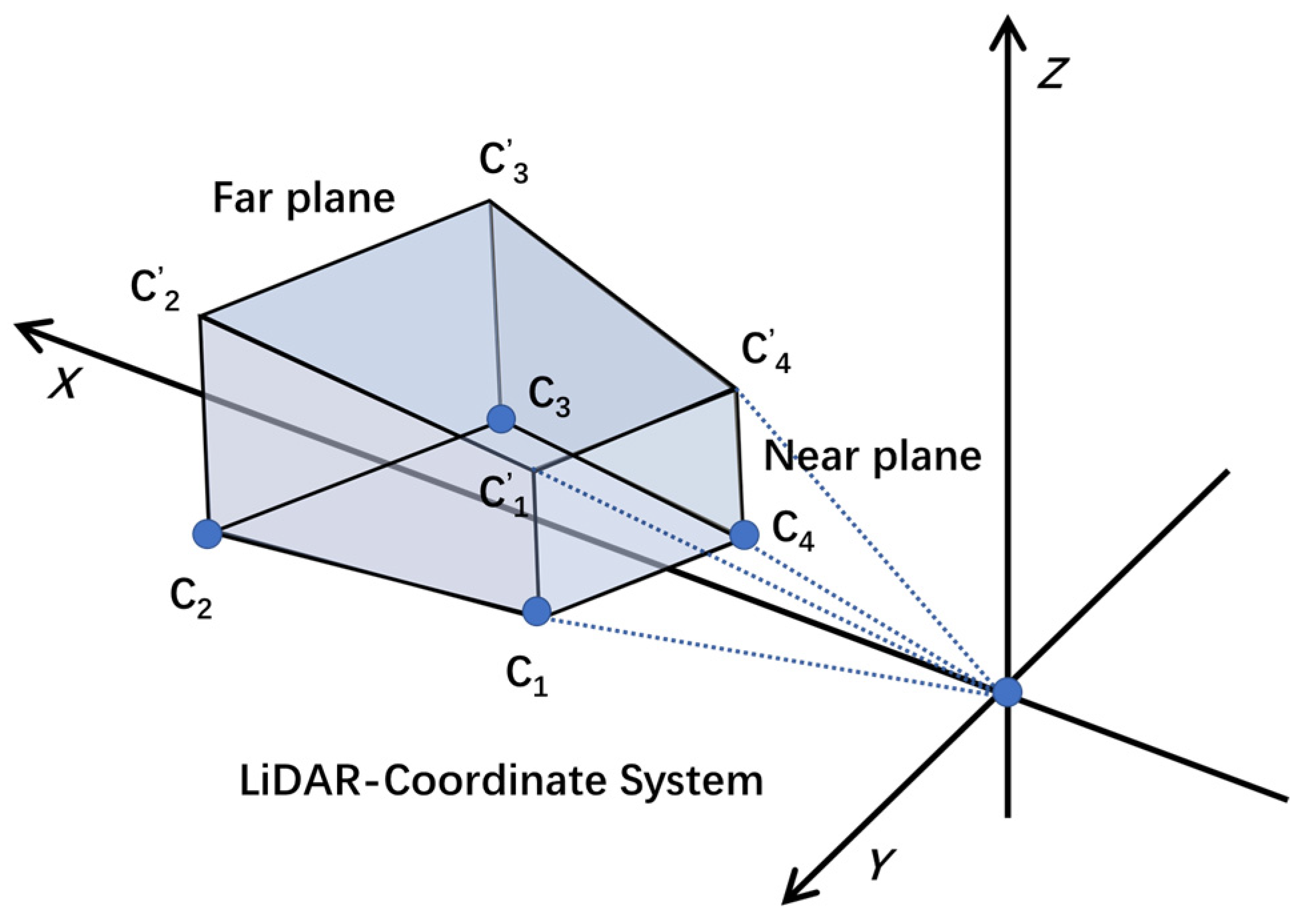
• Projecting the quadrangular prism to the plane coordinate system O-XY. The purpose of this is to simplify the origin model;
• Projecting the corners in far plane to Y-axis and the corresponding points are expressed as V₁ and V₂, as shown in Figure 3;
• According to location of 90° FoV, delimiting the rectangular FoV R-V₁C₂C₃V₂ to get the object attributes within the perspective range;
• Re-adjustment of the FoV is undertaken to optimize the detection range based on the voxel size. Extracting the X_min, Y_min, X_max and Y_max from R-V₁C₂C₃V₂ and setting the difference divided by the voxel size is a multiple of 16.

The backward detection can be seen as rotating the input point clouds 180° for the second detection. Like forward detection, its detection range is calculated by transforming V₁ and V₂ to V₃ and V₄. The formula for the point transformation is as follows:

$$\left[\begin{array}{c}{x}^{\prime }\\ y^{\prime }\\ z^{\prime }\\ 1\end{array}\right]=\left[\begin{array}{c}cos\theta \\ sin\theta \\ 0\\ 0\end{array}\begin{array}{c}-sin\theta \\ cos\theta \\ 0\\ 0\end{array}\begin{array}{c}0\\ 0\\ 1\\ 0\end{array}\begin{array}{c}0\\ 0\\ 0\\ 1\end{array}\right]·\left[\begin{array}{c}x\\ y\\ z\\ 1\end{array}\right]$$

(4)

where (x, y, z) is the location before transform, (x′, y′, z′) represents the location after the transform, and θ is the angle of rotation around the Z-axis. Due to all the x-coordinate values of points in this range being less than 0, forward detection is not required to develop in duplicate. The base PointRCNN is redeployed in this range. Furthermore, although the amount of input data has been increased in the whole process, the backward detection has not brought the loss of accuracy. At the same time, the backward detection can detect effective targets in front and rear of the roadside LiDAR, thus effectively improving the detection performance of roadside LiDAR and providing more information for roadside perception.

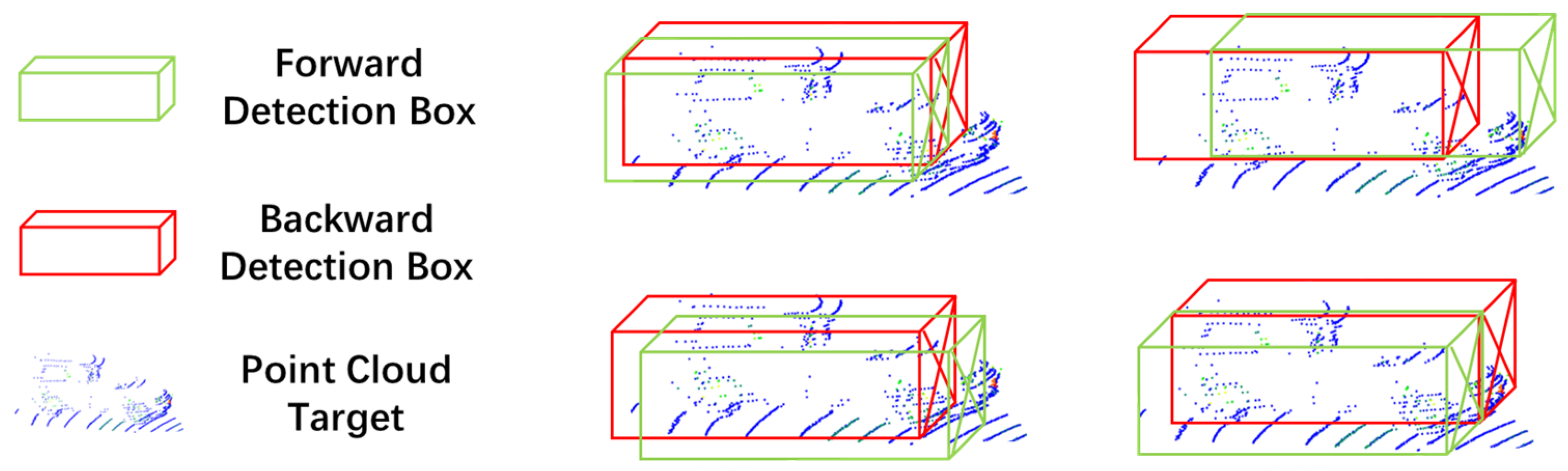
3.3. Overlapping Object Estimation and Removal

After making the omnidirectional detection, forward and backward results can be represented as S₁ and S₂, respectively. To fuse two parts of objects, novel overlapping object estimation and removing methods are designed. Different from traditional point cloud splice or image stitching by using joint points, this method is to apply detection results to conduct later stitching. The entire procedure uses unified data with different ranges and results to fuse non-overlapping objects. The forward and backward detection results are still under the same coordinate system to obtain the final results.

This estimation and removal method is not only adding S₁ and S₂, but it focuses on the problem of multiple detections of the same object across different FoVs (near the seam). When objects pass the front and back regions, point clouds are split into two parts. The PointRCNN can detect the positive object in each part. However, detection results are a false positive for the omnidirectional FoV, which leads to the problem with repeated detection. Then the same target will appear in S₁ and S₂ simultaneously, as shown in Figure 4.

To address the overlapping problem, CD_IoU is designed for overlapping object estimation and removal. IoU is the most popular evaluation metric for bounding box regression in many 2D/3D detection tasks [41]. It usually works when the bounding boxes overlap, which can be represented as:

$$IoU=\frac{\left|B\cap B_{gt}\right|}{\left|B\cup B_{gt}\right|}$$

(5)

where B_gt = {x_gt, y_gt, w_gt, h_gt} indicates the labeled real box, and B = {x, y, w, h} is the predicted box. However, IoU cannot reflect the box distances from each other [42]. Meanwhile, no more labeled boxes are provided in the rectangular FoV. Thus, traditional IoU cannot be applied to describe the degree of overlapping objects from forward and back detection. This paper further proposes a general extension to IoU, namely Center Distance IoU to integrate center-to-center distance and length-to-width ratio. Firstly, the center points of boxes are reduced to 2D points. Euclidean distance is attained by:

$$d(c_1,c_2)=\sqrt{{(x_f-x_b)}^2+{(y_f-y_b)}^2}$$

(6)

where C₁ (x_f, y_f) and C₂ (x_b, y_b) are center points from forward and backward detection boxes. It is apparent that overlapping areas can reduce length or width of no overlapping parts. Specifically, overlapping parts at different angles still reduce the bounding box size of no overlapping parts. The length and width between no overlapping boxes are always larger than overlapping boxes as shown in Figure 5.

$$L_0^{\prime }=L_0-\Delta l(\Delta l\le L_0)$$

(7)

$$W_0^{\prime }=W_0-\Delta w(\Delta w\le W_0)$$

(8)

where L₀ and W₀ are origin detection sizes of boxes, ∆l and ∆w represent the reduction size, $L_0^{\prime }$ and $W_0^{\prime }$ are no overlapping sizes. The CD_IoU can be defined as:

$$C{D}_{IoU}=\frac{1}{2}\left(\frac{l_f+l_b}{2d(c_1,c_2)}+\frac{w_f+w_b}{2d(c_1,c_2)}\right)$$

(9)

where l_f, l_b, w_f, and w_b denote the length and width of B_f and B_b, respectively. The relationships among the above variables are demonstrated in Figure 5.

For CD_IoU, in the case when B_f and B_b overlap exactly, CD_IoU = 0. When the input target bounding boxes partially overlap, the further the distance between the center points, the closer CD_IoU is to 1. If there is no overlap between B_f and B_b, CD_IoU > 1. According to the value of CD_IoU, overlapping object estimation can be implemented automatically. Moreover, the score in Table 1 is used as a metric to remove false positive targets. Different from the general overlap problems, most of the bounding boxes have been refined by PointRCNN in stage-2, and the angle and size are close to the real objects. Thus, the removal method traverses the score of overlapping objects to retain the bounding boxes with higher confidence. Algorithm 1 summarizes the overall procedure of estimation and removal of overlapping objects.

Algorithm 1 Duplicate target estimation and removal

input: Detection result sets S1 (the front frames set) and S2 (the back frames set).

output: A non-repeated data set S3 with 360°.

1  for the cycle in length(S1) do: 2    for the single frame detection result s in S1 and S2 do:        Build empty lists S1_frame and S2_frame to save each frame data. 3     if s[frame] = cycle do:        set the uniform data format for s;        add s to S1_frame or S2_frame. 4    end for

5    Build an empty list del_list to store the indexes of duplicate targets.

6    for each target s1 in S1 do: 7     for each target s2 in S2 do:          Calculating CDIoU(s1,s2) 8       if CDIoU(s1,s2) ≤ 1 do:          s1 and s2 overlap.          Select the index of Min[score(s1), score(s2)] to save in the del_list. 9       else do:           No overlap between s1 and s2. 10     end for 11     Remove multiple elements in the del_list. 12    end for

13    Delete elements in the del_list from S1 and S2.

14    S3 = S1 + S2 15  end for 16  return S3.

4. Experiments

In this section, PointRCNN was trained and evaluated on the KITTI dataset. The experiments were designed to verify the point cloud stitching method. The whole process was performed on a laptop with Ubuntu 18.04 and Robotics Operating System. The GPU was GeForce RTX 1650 and RAM size was 32 GB.

4.1. KITTI Dataset

The KITTI dataset was proposed by Karlsruhe Institute of Technology and Toyota Technological Institute in Chicago to support 3D object detection, 3D tracking, optical flow, and visual odometry tasks. The classes of raw data set are divided into three categories including: ‘Car’, ‘Pedestrian’, and ‘Cyclist’. Raw point cloud data are shown in Figure 6. According to the occlusion and truncation levels, the dataset was grouped into three difficulty levels (easy, moderate, and hard) for each category. The minimum height of the bounding box in easy difficulty level is 40 Px, and the maximum truncation degree is 15%. In the moderate difficulty level, the minimum height of the bounding box is 25 Px, and the maximum truncation degree is 30%. The minimum height of the bounding box in hard level is 25 Px and the maximum truncation degree reaches 50% [43]. The KITTI dataset was divided into 7481 training samples and 7518 testing samples. The PointRCNN in this paper was trained for 500 rounds with an initial learning rate of 0.01, and the batch size was 2.

4.2. Model Evaluation

Among various evaluation metrics, mean Average Precision (mAP) is a commonly used metric for object detection. MAP can be calculated by the Precision–Recall curve, where Precision and Recall can be defined as:

$$Precision=\frac{TP}{TP+FP}$$

(10)

$$Recall=\frac{TP}{TP+FN}$$

(11)

where TP and FP denote true and false positive samples, and FN is the number of false negative samples.

On this basis, a function p(r) of Recall r can be obtained [44]. The 11-point Interpolated Average Precision metric is used to calculate the Average Precision (AP) on each difficulty class as below:

$${AP|}_R=\frac{1}{R}{\displaystyle \sum _{r\in R}p(r)}$$

(12)

where R = R₁₁ = {0, 0.1, 0.2, …, 1}. In this paper, R₄₀ with 41 sub-sampling points [44] was proposed to replace R₁₁, and R₄₀ = {1/40, 2/40, 3/40, …, 1} can eliminate the error encountered and provided more accurate results. Moreover, AP was evaluated from the following four aspects: 2D Bounding Box (bbox), Bird’s Eye View (bev), 3D Bounding Box (3d), and Average Orientation Similarity (aos).

4.3. Results and Discussion

In this paper, the labeled data in the KITTI dataset were utilized and divided it into training (3712 samples) and evaluation sets (3769 samples). For the car class, IoU is set to 0.70 and 0.50, respectively; For pedestrians and cyclists, since their volume is relatively small and generated fewer points, IoU is set to 0.50 and 0.25. Meanwhile, due to less labels in the testing dataset, it is necessary to use the parts of training data to evaluate the algorithm. The performance of PointRCNN in different classes with different IoU is shown in

Table 2. The Performance of PointRCNN in the car class of KITTI with different IoU.

		Easy (Imin = 0.70)	Moderate (Imin = 0.70)	Hard (Imin = 0.70)	Easy (Imin = 0.70)	Moderate (Imin = 0.50)	Hard (Imin = 0.50)
APR11 (Car)	bbox	90.7746	89.6528	89.1511	90.7746	89.6528	89.1511
	bev	90.0448	87.2562	86.4370	90.7395	89.8508	89.5665
	3d	88.9404	78.6675	77.8114	90.7395	89.8258	89.5203
	aos	90.76	89.55	88.98	90.76	89.55	88.98
APR40 (Car)	bbox	96.4271	92.8655	90.5181	96.4271	92.8655	90.5181
	bev	93.1580	88.9119	86.7579	96.4536	95.1651	92.9492
	3d	91.3287	80.5840	78.1417	96.4313	95.0479	92.8361
	aos	96.41	92.74	90.34	96.41	92.74	90.34

,

Table 3. The Performance of PointRCNN in the pedestrian class of KITTI with different IoU.

		Easy (Imin = 0.50)	Moderate (Imin = 0.50)	Hard (Imin = 0.50)	Easy (Imin = 0.50)	Moderate (Imin = 0.25)	Hard (Imin = 0.25)
APR11 (Pedestrian)	bbox	73.5689	66.1255	62.2895	73.5689	66.1255	62.2895
	bev	67.1253	58.8610	53.3021	82.0378	74.9234	67.0553
	3d	61.8900	54.4388	50.1242	81.9940	74.7333	66.9421
	aos	70.86	63.01	59.00	70.86	63.01	59.00
APR40 (Pedestrian)	bbox	74.8557	67.7918	61.0786	74.8557	67.7918	61.0786
	bev	66.1146	58.1660	51.4365	82.8676	76.0780	68.8326
	3d	62.8512	54.9202	47.9085	82.7933	74.8970	67.6176
	aos	71.85	64.21	57.60	71.85	64.21	57.60

and

Table 4. The Performance of PointRCNN in the cyclist class of KITTI with different IoU.

		Easy (Imin = 0.50)	Moderate (Imin = 0.50)	Hard (Imin = 0.50)	Easy (Imin = 0.50)	Moderate (Imin = 0.25)	Hard (Imin = 0.25)
APR11 (Cyclist)	bbox	89.6212	76.3985	70.1547	89.6212	76.3985	70.1547
	bev	85.7266	71.9324	66.3024	88.4910	74.5981	68.5349
	3d	85.0175	66.8832	64.3491	88.4910	74.5981	68.5349
	aos	89.54	75.90	69.74	89.54	75.90	69.74
APR40 (Cyclist)	bbox	94.9042	77.2506	72.8562	94.9042	77.2506	72.8562
	bev	90.3609	71.2446	68.1587	93.5190	75.2005	70.8290
	3d	87.6985	68.6195	64.1195	93.5190	75.2005	70.8290
	aos	94.82	76.71	72.33	94.82	76.71	72.33

.

According to the detailed detection results, PointRCNN has better performance on the car class under different difficulty levels. Due to the smaller size, the perception was somewhat reduced for pedestrians and cyclists. To show performance of the model as intuitive as possible the detection results were comparatively visualized as shown in Figure 7. The above parts in Figure 7 are corresponding images, and the lower parts in Figure 7 are detection results in point clouds. Since the limitation of FoV and dataset, the base trained model only performed in a small detection range.

The proposed method in this paper was further applied to each frame of point clouds. Two sets of virtual environments in Anaconda were built to run the detection model. Based on the location of roadside LiDAR, forward and backward detection with a range of 0°–180° were implemented in parallel. The results were saved with the same time of calculation. The two sets of 180° results from the same point cloud frame were provided in Figure 8. One is forward detection results, and another is backward results.

It is obvious that detection results are in the same environment and sensor location, but the detection range is different, therefore making the stitching method necessary. Coarse stitching was made for two sets of point clouds as in Figure 9. The results from the same coordinate system were combined in a set of the omnidirectional detection results. Compared with the previous approaches, the stitching method obtained more detection results to be merged, but no additional point clouds were added. Specifically, more detailed and valid objects can be detected at 360° by base model that was trained by labeled targets. The stitching method in this paper is an effective way that can further expand detection range by associating results to the same coordinate system. It should be noted that overlapping targets were added near the stitching. By utilizing estimation and removing methods, the CD_IoU of each of bounding boxes could be calculated. The final stitch data are shown in Figure 10, where each object is highlighted by a green bounding box. It shows that the proposed method can stitch the point cloud correctly based on detection results. The redundant information is removed successfully by multi-detection on the same frame, and the true positive results with higher confidence scores are retained completely. A smooth transition is realized when the same target crossed FoVs, and it can generate more meaningful results for roadside perception.

In addition, the roadside LiDAR was temporarily installed on a tripod for this study, as shown in Figure 11a. The detection results are also described by green bounding boxes in Figure 11b–e. Meanwhile, multiple existing methods (PointRCNN [36], PV-RCNN [34], SECOND [7] and Part-A2-Free [45]) were tested on same collected point cloud data, respectively. In

Table 5. The Performance of different detection algorithms.

	PointRCNN (Base)	PV-RCNN	SECOND	Part-A2-Free	Ours
Training time	3 h	5 h	1.7 h	3.8 h	3 h
Running time	120.548 s	102.653 s	50.595 s	93.343 s	121.469 s
Detection range	Front FoV	Front FoV	Front FoV	Front FoV	360° FoV
AP	88.9404	89.3476	88.6137	89.1192	88.9404
Output objects	4306	6094	8051	6259	7628

, the performances of different detection algorithms with training time, running time, detection range, AP and output objects were further compared. The AP (3d) under easy conditions for the car class was selected to represent the accuracy level of models. All the algorithms showed similar performance in the AP, but the proposed method (88.9404) is higher than SECOND (88.6137). The training time of ours is lower than most of the methods, which means an effective detection model can be obtained for roadside perception as soon as possible. It should be noted that the total training and running time of the proposed method was performed at a similar level with the base PointRCNN. This is because the stitching method was based on PointRCNN improvement, where forward and backward detection can be conducted in parallel with a high efficiency. Omnidirectional detection results can be generated in the same environment without more computational resources such as larger memory consumption. Even though the time this stitching algorithm takes was not shorter than other models, more precise and robust detection was provided, as can be seen from visualization results. In Figure 11b–e, objects can be detected but the cover range was limited to the front FoV. Some close targets with sufficient features were not labeled due to being beyond the range of the front FoV, which cannot meet the needs of roadside perception. In addition, a maximum of 8051 objects were outputted by other models within the limitations of the search range, but it clearly did not properly evaluate the quality of an algorithm. It can be observed that some results are false positive objects in Figure 11b–e, especially the results provided by SECOND and Part-A2-Free. Conversely, our method could output true positive objects, as many as possible, as Figure 11f described. The near, distant and back targets could be included in the detection results. Taken together, the proposed stitching method can support the perception tasks of roadside LiDAR., which could produce more accurate results in 360° FoV with less training time.

5. Conclusions

This paper introduces a 3D point cloud stitching method for object detection with wide FoV using Roadside LiDAR, which contains an object detection framework for point clouds, an omnidirectional detection results generating module, and a novel approach for overlapping object estimation and removal. Based on the experiments and visualization, the proposed approach could successfully stitch multiple sets of the detection results in a small range generated by the same LiDAR sensor. After optimizing the results, larger detection can be realized without generating overlapping targets. Stitching also provides a cost-efficient solution to object detection using roadside LiDAR. This addresses the problem of perception and application using popular vehicle datasets in the case of a missing roadside LiDAR dataset.

Some limitations of this paper still exist. The overlapping object estimation and removal method is difficult to work out without any error, particularly in areas with less object spacing such as large parking lots. The current algorithm is still expected to optimize thresholds of CD_IoU. If a real-time and integrated system could be constructed, the computations involved in object detection and stitching will be carried out in real time. Furthermore, this paper did not provide an effective way to overcome the effects of bad weather that can limit the performance of algorithms. Noise points may have contributed to wrong forward and back detections under rainy and snowy weather. Further studies can consider making data processing and analysis in these realistic scenarios. Experiments also reveal that some voxel-based methods have particular advantages for running time. Future work should not be restricted to only point-based detection models; efforts will also need to be made to provide fast and accurate 3D detection using other methods.

References

1. Chen, X.; Ma, H.; Wan, J.; Li, B.; Xia, T. Multi-view 3d object detection network for autonomous driving. In Proceedings of the IEEE Conference on Computer Vision and Pattern Recognition, Honolulu, HI, USA, 21–26 July 2017; pp. 1907–1915. [Google Scholar]
2. Wu, J.; Xu, H.; Zheng, Y.; Zhang, Y.; Lv, B.; Tian, Z. Automatic vehicle classification using roadside LiDAR data. Transp. Res. Rec. 2019, 2673, 153–164. [Google Scholar] [CrossRef]
3. Guo, Y.; Wang, H.; Hu, Q.; Liu, H.; Liu, L.; Bennamoun, M. Deep learning for 3d point clouds: A survey. IEEE Trans. Pattern Anal. Mach. Intell. 2020, 43, 4338–4364. [Google Scholar] [CrossRef]
4. Tang, H.; Liu, Z.; Li, X.; Lin, Y.; Han, S. Torchsparse: Efficient point cloud inference engine. Proc. Mach. Learn. Syst. 2022, 4, 302–315. [Google Scholar]
5. Zimmer, W.; Ercelik, E.; Zhou, X.; Ortiz, X.J.D.; Knoll, A. A survey of robust 3d object detection methods in point clouds. arXiv 2022, arXiv:2204.00106. [Google Scholar]
6. Wu, J.; Tian, Y.; Xu, H.; Yue, R.; Wang, A.; Song, X. Automatic ground points filtering of roadside LiDAR data using a channel-based filtering algorithm. Opt. Laser Technol. 2019, 115, 374–383. [Google Scholar] [CrossRef]
7. Yan, Y.; Mao, Y.; Li, B. Second: Sparsely embedded convolutional detection. Sensors 2018, 18, 3337. [Google Scholar] [CrossRef] [Green Version]
8. Qian, R.; Lai, X.; Li, X. 3d object detection for autonomous driving: A survey. arXiv 2021. [Google Scholar] [CrossRef]
9. Mao, J.; Shi, S.; Wang, X.; Li, H. 3d object detection for autonomous driving: A review and new outlooks. arXiv 2022, arXiv:2206.09474. [Google Scholar]
10. Li, J.; Hu, Y. Dpointnet: A density-oriented pointnet for 3d object detection in point clouds. arXiv 2021, arXiv:2102.03747. [Google Scholar]
11. Zhao, J.; Xu, H.; Liu, H.; Wu, J.; Zheng, Y.; Wu, D. Detection and tracking of pedestrians and vehicles using roadside LiDAR sensors. Transp. Res. Part C Emerg. Technol. 2019, 100, 68–87. [Google Scholar] [CrossRef]
12. Wu, J. An automatic procedure for vehicle tracking with a roadside LiDAR sensor. Inst. Transp. Eng. ITE J. 2018, 88, 32–37. [Google Scholar]
13. Wu, J.; Xu, H.; Tian, Y.; Pi, R.; Yue, R. Vehicle detection under adverse weather from roadside LiDAR data. Sensors 2020, 20, 3433. [Google Scholar] [CrossRef]
14. Wu, J.; Xu, H.; Zhao, J. Automatic lane identification using the roadside LiDAR sensors. IEEE Intell. Transp. Syst. Mag. 2020, 12, 25–34. [Google Scholar] [CrossRef]
15. Wu, J.; Xu, H.; Lv, B.; Yue, R.; Li, Y. Automatic ground points identification method for roadside LiDAR data. Transp. Res. Rec. J. Transp. Res. Board 2019, 2673, 140–152. [Google Scholar] [CrossRef]
16. Caesar, H.; Bankiti, V.; Lang, A.H.; Vora, S.; Liong, V.E.; Xu, Q.; Krishnan, A.; Pan, Y.; Baldan, G.; Beijbom, O. NuScenes: A multimodal dataset for autonomous driving. arXiv 2020, arXiv:1903.11027. [Google Scholar]
17. Liao, Y.; Xie, J.; Geiger, A. Kitti-360: A novel dataset and benchmarks for urban scene understanding in 2d and 3d. IEEE Trans. Pattern Anal. Mach. Intell. 2022. [Google Scholar] [CrossRef]
18. Sun, P.; Kretzschmar, H.; Dotiwalla, X.; Chouard, A.; Patnaik, V.; Tsui, P.; Guo, J.; Zhou, Y.; Chai, Y.; Caine, B. Scalability in perception for autonomous driving: Waymo open dataset. In Proceedings of the IEEE/CVF Conference on Computer Vision and Pattern Recognition, ELECTR NETWORK, Seattle, WA, USA, 13–19 June 2020; pp. 2446–2454. [Google Scholar]
19. Xiang, T.-Z.; Xia, G.-S.; Bai, X.; Zhang, L. Image stitching by line-guided local warping with global similarity constraint. Pattern Recognit. 2018, 83, 481–497. [Google Scholar] [CrossRef] [Green Version]
20. Zaragoza, J.; Tat-Jun, C.; Tran, Q.H.; Brown, M.S.; Suter, D. As-projective-as-possible image stitching with moving DLT. IEEE Trans. Pattern Anal. Mach. Intell. 2014, 36, 1285–1298. [Google Scholar]
21. Li, N.; Liao, T.; Wang, C. Perception-based seam cutting for image stitching. Signal Image Video Process. 2018, 12, 967–974. [Google Scholar] [CrossRef]
22. Chen, X.; Yu, M.; Song, Y. Optimized seam-driven image stitching method based on scene depth information. Electronics 2022, 11, 1876. [Google Scholar] [CrossRef]
23. Shi, Z.; Wang, P.; Cao, Q.; Ding, C.; Luo, T. Misalignment-eliminated warping image stitching method with grid-based motion statistics matching. Multimed. Tools Appl. 2022, 81, 10723–10742. [Google Scholar] [CrossRef]
24. Zakaria, M.A.; Kunjunni, B.; Peeie, M.H.B.; Papaioannou, G. Autonomous shuttle development at university Malaysia Pahang: LiDAR point cloud data stitching and mapping using iterative closest point cloud algorithm. In Towards Connected and Autonomous Vehicle Highways; Umar, Z.A.H., Fadi, A., Eds.; Springer: Cham, Switzerland, 2021; pp. 281–292. [Google Scholar]
25. Ibisch, A.; Stümper, S.; Altinger, H.; Neuhausen, M.; Tschentscher, M.; Schlipsing, M.; Salinen, J.; Knoll, A. Towards autonomous driving in a parking garage: Vehicle localization and tracking using environment-embedded LiDAR sensors. In Proceedings of the 2013 IEEE Intelligent Vehicles Symposium (IV), Gold Coast, Australia, 23–26 June 2013; pp. 829–834. [Google Scholar]
26. Sun, H.; Han, J.; Wang, C.; Jiao, Y. Aircraft model reconstruction with image point cloud data. In Proceedings of the 2018 IEEE 3rd International Conference on Cloud Computing and Big Data Analysis (ICCCBDA), Chengdu, China, 20–22 April 2018; pp. 322–325. [Google Scholar]
27. Wu, J.; Song, X. Review on development of simultaneous localization and mapping technology. J. Shandong Univ. (Eng. Sci.) 2021, 51, 16–31. [Google Scholar]
28. Yao, S.; AliAkbarpour, H.; Seetharaman, G.; Palaniappan, K. City-scale point cloud stitching using 2d/3d registration for large geographical coverage. In Proceedings of the International Conference on Pattern Recognition, Virtual Event, 10–15 January 2021; pp. 32–45. [Google Scholar]
29. Lv, B.; Xu, H.; Wu, J.; Tian, Y.; Tian, S.; Feng, S. Revolution and rotation-based method for roadside LiDAR data integration. Opt. Laser Technol. 2019, 119, 105571. [Google Scholar] [CrossRef]
30. Wu, J.; Xu, H.; Zheng, Y.; Tian, Z. A novel method of vehicle-pedestrian near-crash identification with roadside LiDAR data. Accid. Anal. Prev. 2018, 121, 238–249. [Google Scholar] [CrossRef]
31. Zhang, Y.; Xu, H.; Wu, J. An automatic background filtering method for detection of road users in heavy traffics using roadside 3-d LiDAR sensors with noises. IEEE Sens. J. 2020, 20, 6596–6604. [Google Scholar] [CrossRef]
32. Yang, Z.; Sun, Y.; Liu, S.; Jia, J. 3dssd: Point-based 3d single stage object detector. In Proceedings of the 2020 IEEE/CVF Conference on Computer Vision and Pattern Recognition (CVPR), Seattle, WA, USA, 13–19 June 2020; pp. 11040–11048. [Google Scholar]
33. Shi, W.; Rajkumar, R. Point-gnn: Graph neural network for 3d object detection in a point cloud. In Proceedings of the IEEE/CVF Conference on Computer Vision and Pattern Recognition, ELECTR NETWORK, Seattle, WA, USA, 13–19 June 2020; pp. 1711–1719. [Google Scholar]
34. Shi, S.; Guo, C.; Jiang, L.; Wang, Z.; Shi, J.; Wang, X.; Li, H. Pv-rcnn: Point-voxel feature set abstraction for 3d object detection. In Proceedings of the IEEE/CVF Conference on Computer Vision and Pattern Recognition, Seattle, WA, USA, 14–19 June 2020; pp. 10529–10538. [Google Scholar]
35. Wang, S.; Pi, R.; Li, J.; Guo, X.; Lu, Y.; Li, T.; Tian, Y. Object tracking based on the fusion of roadside LiDAR and camera data. IEEE Trans. Instrum. Meas. 2022, 71, 1–14. [Google Scholar] [CrossRef]
36. Shi, S.; Wang, X.; Li, H. Pointrcnn: 3d object proposal generation and detection from point cloud. In Proceedings of the IEEE/CVF Conference on Computer Vision and Pattern Recognition, Long Beach, CA, USA, 16–20 June 2019; pp. 770–779. [Google Scholar]
37. Qi, C.R.; Yi, L.; Su, H.; Guibas, L.J. Pointnet++: Deep hierarchical feature learning on point sets in a metric space. In Advances in Neural Information Processing Systems 30; Curran Associates, Inc.: Long Beach, CA, USA, 2017. [Google Scholar]
38. OpenPCDet Development Team. Openpcdet: An Open-Source Toolbox for 3D Object Detection from Point Clouds. 2020. Available online: https://github.com/open-mmlab/OpenPCDet (accessed on 1 December 2022).
39. Geiger, A.; Lenz, P.; Urtasun, R. Are we ready for autonomous driving? The kitti vision benchmark suite. In Proceedings of the 2012 IEEE Conference on Computer Vision and Pattern Recognition, Providence, RI, USA, 16–21 June 2012; pp. 3354–3361. [Google Scholar]
40. Luo, Y.; Qin, H. 3D Object Detection Method for Autonomous Vehicle Based on Sparse Color Point Cloud. Automot. Eng. 2021, 43, 492–500. [Google Scholar]
41. Zheng, Z.; Wang, P.; Liu, W.; Li, J.; Ye, R.; Ren, D. Distance-iou loss: Faster and better learning for bounding box regression. In Proceedings of the AAAI Conference on Artificial Intelligence, New York, NY, USA, 7–12 February 2020; pp. 12993–13000. [Google Scholar]
42. Rezatofighi, H.; Tsoi, N.; Gwak, J.; Sadeghian, A.; Reid, I.; Savarese, S. Generalized intersection over union: A metric and a loss for bounding box regression. In Proceedings of the 2019 IEEE/CVF Conference on Computer Vision and Pattern Recognition (CVPR), Long Beach, CA, USA, 16–20 June 2019; pp. 658–666. [Google Scholar]
43. Liu, L.; He, J.; Ren, K.; Xiao, Z.; Hou, Y. A LiDAR–camera fusion 3d object detection algorithm. Information 2022, 13, 169. [Google Scholar] [CrossRef]
44. Simonelli, A.; Bulo, S.R.; Porzi, L.; López-Antequera, M.; Kontschieder, P. Disentangling monocular 3d object detection. In Proceedings of the IEEE/CVF International Conference on Computer Vision, Seoul, Republic of Korea, 27 October–2 November 2019; pp. 1991–1999. [Google Scholar]
45. Shi, S.; Wang, Z.; Shi, J.; Wang, X.; Li, H. From points to parts: 3d object detection from point cloud with part-aware and part-aggregation network. IEEE Trans. Pattern Anal. Mach. Intell. 2020, 43, 2647–2664. [Google Scholar] [CrossRef]
Figure 1. The framework of the proposed stitching method.
Electronics 12 00703 g001
Figure 2. The viewing frustum of the camera.
Electronics 12 00703 g002
Figure 3. The range and degrees of forward and backward detection.
Electronics 12 00703 g003
Figure 4. Examples of multiple detections of the same object across the seam.
Electronics 12 00703 g004
Figure 5. The reduction in length and width between the overlapping boxes.
Electronics 12 00703 g005
Figure 6. The example of raw point clouds in KITTI dataset.
Electronics 12 00703 g006
Figure 7. The base detection results from PointRCNN.
Electronics 12 00703 g007
Figure 8. The broad detection results from PointRCNN.
Electronics 12 00703 g008
Figure 9. The omnidirectional detection results from PointRCNN.
Electronics 12 00703 g009
Figure 10. The final detection results by refined point cloud stitching.
Electronics 12 00703 g010
Figure 11. Sensors and detection results of different the methods: (a) Roadside LiDAR; (b) PointRCNN (base); (c) PV-RCNN; (d) SECOND; (e) Part-A2-Free; (f) The proposed method.
Electronics 12 00703 g011