Article

Towards Deploying DNN Models on Edge for Predictive Maintenance Applications

1
System Design Department, IMMS Institut für Mikroelektronik- und Mechatronik-Systeme Gemeinnützige GmbH (IMMS GmbH), Ehrenbergstraße 27, 98693 Ilmenau, Germany
2
Department of Computer and Electrical Engineering, Mid Sweden University, Holmgatan 10, 851 70 Sundsvall, Sweden
*
Author to whom correspondence should be addressed.
Electronics 2023, 12(3), 639; https://doi.org/10.3390/electronics12030639
Submission received: 9 January 2023 / Revised: 21 January 2023 / Accepted: 23 January 2023 / Published: 27 January 2023
(This article belongs to the Section Artificial Intelligence)

Abstract

:
Almost all rotating machinery in the industry has bearings as their key building block and most of these machines run 24 × 7. This makes bearing health prediction an active research area for predictive maintenance solutions. Many state of the art Deep Neural Network (DNN) models have been proposed to solve this. However, most of these high performance models are computationally expensive and have high memory requirements. This limits their use to very specific industrial applications with powerful hardwares deployed close the the machinery. In order to bring DNN-based solutions to a potential use in the industry, we need to deploy these models on Microcontroller Units (MCUs) which are cost effective and energy efficient. However, this step is typically neglected in literature as it poses new challenges. The primary concern when inferencing the DNN models on MCUs is the on chip memory of the MCU that has to fit the model, the data and additional code to run the system. Almost all the state of the art models fail this litmus test since they feature too many parameters. In this paper, we show the challenges related to the deployment, review possible solutions and evaluate one of them showing how the deployment can be realized and what steps are needed. The focus is on the steps required for the actual deployment rather than finding the optimal solution. This paper is among the first to show the deployment on MCUs for a predictive maintenance use case. We first analyze the gap between State Of The Art benchmark DNN models for bearing defect classification and the memory constraint of two MCU variants. Additionally, we review options to reduce the model size such as pruning and quantization. Afterwards, we evaluate a solution to deploy the DNN models by pruning them in order to fit them into microcontrollers. Our results show that most models under test can be reduced to fit MCU memory for a maximum loss of 3 % in average accuracy of the pruned models in comparison to the original models. Based on the results, we also discuss which methods are promising and which combination of model and feature work best for the given classification problem.

1. Introduction

Rotating machinery is an inevitable part of industrial infrastructure and bearings are a key component in rotating machinery. Industrial machines are typically functional all around the year and an unwanted interruption in their operation due to faults in the bearings can be costly. Over time, certain extreme operating temperature or load conditions can lead to bearing failures. It is important to identify such failures in order to schedule timely maintenance [1] with minimal or almost no loss in operation pipeline. So far, the most common solution to this problem is to replace the bearings based on life cycle estimations. This leads to two possible unoptimized results. One is the replacement of still good bearings which would be operational for some time. The other is a sudden shut down in the operation line because of an unexpected fault occurring before the next maintenance cycle.
A considerable amount of research was done in the area of predictive maintenance (Pdm) to identify the defects, classify their type, or predict remaining useful life (RUL) of a bearing in a system with rotating machinery. Pdm is tackled using both traditional ML and end-to-end Deep Neural Network (DNN). While traditional ML involves an expensive feature engineering phase and a specific classifier, DNN approaches to identify the relevant features during training themselves. Most of the time, both methods are explored on public benchmark data to evaluate the performance of a solution and show promising results. However, the actual integration of a solution into the industrial process remains open. The main reasons are that these models are typically run on specialized hardware or servers in the cloud, while industrial partners prefer local on premise processing to ensure timely decisions and security. To cover this, the models should be executed closer to the actual machine and thus be realized as Edge-AI.
Shifting the execution of ML models to the edge for predictive maintenance is still an open problem and is typically not addressed by any SOTA works in the field of industrial machine diagnosis. In this paper, the term edge is strictly constrained to low power micro controller units (MCUs) rather than Jetson Nano, Raspberry Pi or other similar micro computers with significantly higher computational resources. We chose this definition because MCU-based components are easy to integrate into the machinery. This allows running a ML-model close to the actual industrial process. However, MCUs typically are constrained in computational resources as well as available memory. Therefore, executing SOTA ML-models becomes a challenge since their requirements typically do not match. In this paper, we will first highlight this mismatch and then introduce an approach to reduce the model size and thus mitigate the constraint. Our solution thus enables the integration of ML-solutions into the industrial process. In addition, we will discuss the impact of our approach on model accuracy and highlight further challenges towards the implementation into the machinery.
To prove the insufficiency of the SOTA solutions, we chose a benchmark study [2] as the baseline of our work. Out of the discussed datasets in the study, we selected a public bearing dataset [3] as a base for our work. Regarding the considered models, we follow the benchmark and considered the Autoencoder (AE), its variations Sparse Autoencoder (SAE) and Denoising Autoencoder (DAE) as well as CNN based models (AlexNet, ResNet, LeNet). Though these DNN models are accurate in classifying the type of bearing defect, it was impossible to inference them on MCUs as is.
Therefore, we focus on the deployment of pretrained models, i.e., models are trained on powerful hardware and then transferred together with the trained weights to the target hardware to perform inference. Transferring DNN models to MCUs poses memory problems because DNN models typically have a high number of parameters. In addition, DNN models require lots of computational cycles to get the desired inference result which also makes them power hungry. To solve these problems, we propose a solution to trim the benchmarked Pdm models using state of the art pruning algorithms [4] in order to fit them into MCUs.
In this paper, we present the following contributions:
  • Evaluation of challenges in deploying state of the art DNN models to MCUs
  • Review options to reduce the model size
  • Show the impact of pruning the weights as reduction method on model size and inference time on the MCU
The remainder of the paper is organized as follows. In Section 2, we first give an overview of the models targeting the bearing defect classification problem and then review works targeting model size reduction. Afterwards, we describe our method in Section 3. We introduce the dataset and models used for our study as well as the required fundamentals of the pruning approach. In addition, we give details regarding model training and deployment. Section 4 presents the results of our experiments which are then discussed in Section 5. Finally, the paper is concluded in Section 6 where we also indicate our plans for further studies.

2. Literature Review

In this section, we review a number of state of the art papers, that present approaches to handle bearing health prediction. With the advancement of high end ML libraries like TensorFlow [5], keras and sklearn, it is possible to implement better data analysis algorithms and develop complex models to achieve benchmark results in fault diagnosis. Data driven models have gained popularity with help from such sophisticated APIs. As a result, many solutions to Pdm of bearings or other rotating machinery have been suggested and several different algorithms and flavors exist.
Models like Autoencoders (AEs) have been a popular choice because of their semi-supervised learning approach. The authors in [6] used a customized AE loss function and Artificial Fish Swarm Algorithm (AFSA) for parameter optimization. In [7], the authors introduce stacked AE for bearings functioning at low operating speeds. The Sparse Autoencoder (SAE) was applied for data fusion and feature encoding in [8] before classifying them with Deep Belief Network (DBN). Another variation of SAE called Deep Nonnegativity-Constraint SAE (DNSAE) was applied in [9] to encode features and achieve high diagnosis accuracy even with few labeled dataset. AEs were also used with convolutional layers [10] in some cases to denoise the input. These functional or structural modifications in AE produced better results compared to the general models.
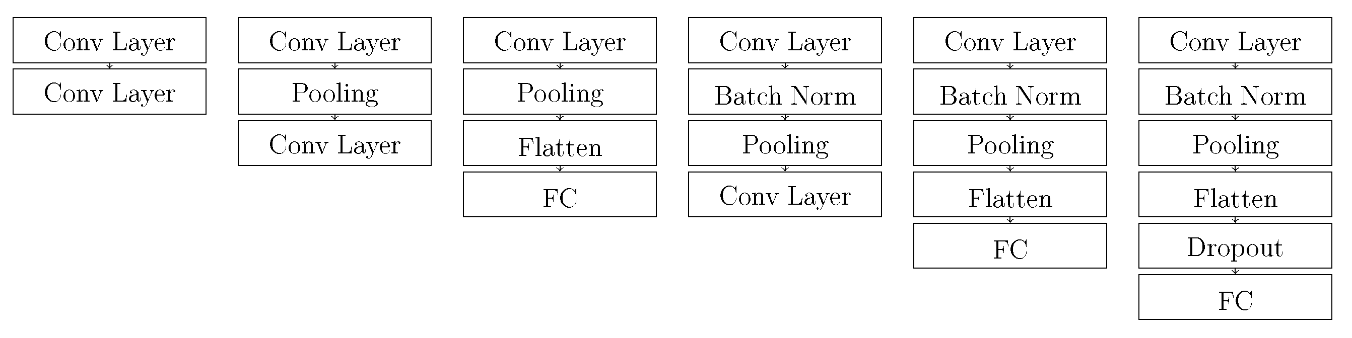
Though AEs had an advantage of semi supervised learning and feature encoding capabilities, Convolutional Neural Networks (CNNs) outperform them in feature extraction with less trainable parameters. CNNs are used extensively in image classification as they can extract different types of features using stacked filters. One option to feed vibration signals into the CNN is to convert the signals to 2-D image and use this as input for the CNN. This allows the reuse of popular models from image classification. In [11], the authors use Empirical Mode Decomposition (EMD) and CNN for signal analysis and feature extraction. EMD can decompose the signal into its components and CNN extracts the spatial features in the signal components. The extracted features are fused and used to classify faults. In [12,13], the authors used CNNs as replacement of hand crafted feature extraction.
Different structural formulations of CNNs have been experimented with bearing datasets for predictive maintenance applications. Different variations of AlexNet [14,15,16,17], ResNet [18,19,20,21,22] and LeNet [23,24] are used in different research works for fault diagnosis of rolling bearing elements. In [14,15], the authors proposed an one dimensional model slightly deeper than the original AlexNet model to enhance the bearing fault classification and compared their model with AlexNet. Instead of this, [17] shows that a AlexNet model can be used by just retraining the fully connected (FC) layers at the end to identify bearing defects. Thermal images were used as input to AlexNet in [16] in order to detect bearing faults.
ResNet models have the potential to provide better diagnostic accuracy without increasing the model depth due to the residual blocks. This makes them interesting candidates for bearing diagnosis. In [18], bearing faults were identified using continuous wavelet transform of raw signals by using pretrained ResNet-50 model with transfer learning. A wavelet transform based intelligent fault classifier for rolling bearing was built in [19]. The classifier is based on ResNet with a new pooling layer. Principal Component Analysis was used in [20] for noise reduction in bearing signals before using them to classify faults using ResNet. In [21], ResNet is used to generalize the bearing fault diagnosis in a more generalized and unified way. A global average pooling layer is used in ResNet instead of multiple FC layer for classification in [22] in order to reduce the parameters.
LeNet is comparatively the shallowest among the three CNN models mentioned here. It is therefore more interesting for inference on MCUs. Different variations of LeNet model have been used i.e., in [23,24] to improve the fault diagnosis results in comparison to the basic LeNet-5. In [23], the authors added convolution and pooling layers and calculated the sensitivity of the pooling operation based on the error. The authors in [24] focus on solving the convergence issue and generalization problem of LeNet-5 architecture. A batch normalization layer after every convolutional layer was added to improve the convergence speed and the one dimensional vibration signal was converted to 2D to improve the diagnosis results. Thus this paper aims at an improvement in model performance while not attempting to actually deploy the model to real hardware.
On one side, most of the research investigating the improvement in predictive maintenance proposed some novelty in model architecture, selection of hyper parameters or dataset preprocessing. On the other side, there has been extensive research in order to reduce the memory and computational requirement of DNN models. This broadly comprises two different strategies, quantization of the weights of the model and pruning the unnecessary weights. The authors in [25,26] proposed automatic model compression strategy in order to structurally prune weights based on Alternating Direction Method of Multipliers and Sparse Connectivity Learning, respectively. In [27], network width search is automated by adding a depth-wise learnable binary convolutional layer. Quantization also reduces the number of flops in the network. A reduction in the number of bits directly accelerates the model inference time. In [28], the authors used a hardware friendly quantization approach which tries to bring best of both uniform and non-uniform quantization. Value aware quantization can reduce the model size more aggressively as shown in [29]. Here, the authors exploited the distribution of weight values to reduce the quantization results.
In summary, the focus of the state of the art work is either on fine tuning the pretrained models or compress the models in order to make them inference friendly. To the best of our knowledge, only few approaches consider the model deployment challenge. Authors in [30] have discussed the cost of two spectral feature extraction methods and their trade offs while inferencing them on MCUs. But it does not involve DNNs and the the problem was addressed only from a theoretical perspective. Another example is described in [31]. The proposed Deployment Oriented to Memory (DORY) tool for DNNs is focused on better memory hierarchy management and deployment on MCUs with less than 1 MB of on-chip SRAM. However, this approach is particularly tuned to Parallel Ultra Low Power Paradigm (PULP) architecture and thus not suitable for general purpose MCUs. In [25], the researchers deploy a pruned model on a smartphone. This shows that pruning is suitable to reduce the model size to fit them into embedded devices. But modern smartphones feature rather powerful hardware and large memory.
Therefore, only powerful embedded hardware has been considered as deployment candidate. Our perspective on Edge AI is inspired by the industrial applications where general purpose MCUs are key to get the models close to the process in an energy-efficient way. Table 1 provides a comparison among the SOTA results and the current work.
Hence, we suggest to investigate whether optimized deep learning models can be practically deployed to general purpose MCUs and thus check if they are feasible in industrial scenarios. Such an analysis is crucial to highlight open gaps towards actual deployment and application of Pdm within industrial machinery.

3. Materials and Methods

3.1. Dataset

There are plenty of public datasets available for bearing condition monitoring and [2] provides a brief explanation of popular datasets as well as classification accuracies achieved by all the six models explained in Section 3.2. We selected XJTU bearing dataset [3] for our experiments. We chose this dataset because all models provide a good accuracy for the problem and thus we can focus on the inference phase showing differences resulting from the deployment.
The dataset contains fifteen run to failure bearing measurements recorded with accelerometers at different load conditions. The majority of the bearing operation duration consists of optimal operable state and only small portion at the end of bearing life shows defect indications. This can be clearly understood form Figure 1 which shows vibration measurement for a bearing for ≈2 h and the defect can be indicated starting from ≈80 min. If the bearing is functional for a long duration, the dataset could be imbalanced as relatively many measurements from the operable state will create a bias and DNN model will not generalize anymore. Such scenarios can introduce the class imbalance problem while training the model. As a solution to that, we selected only the last four minutes of measurement from the bearing lifetime, which is feasible for a task classifying the type of defect. This equalizes the data available from each bearing type irrespective of their operation duration. This is valid since our models are focused on solving a classification problem with respect to different type of defects in the bearings operating at variable conditions.
Each minute of measurement contains 32,768 (≈32k) samples [3]. This is sub sampled by dividing it into sets of m = 1024 samples each, x t R m × 1 . With this sub sampling approach, one minute of measurement yields 32 sets of data from each minute. As we are using last four minutes of data from each bearing lifetime, we have ( 32 × 4 = 128 ) sets of data from each bearing operating at a particular condition. With fifteen such bearings we have 1920 ( n = 128 × 15 ) data samples.
We formulated the collected measurement samples in five different features as discussed in [2].

3.1.1. Time Domain Signals

The time domain signals are the raw measurement collected from the accelerometer shown in Figure 1. With the above sub sampling of the time domain we can formulate a dataset X t R n × m × 1 which can be used as an input to the model. We normalize the signal before using it on any DNN model or for further feature extraction selecting one approach presented in [2]. The time signals X t is normalized using Equation (1) where x i represents one row of X t where as x i μ and x i σ denotes the mean and standard deviation of x i . In the rest of the paper, we do not explicitly mention or denote normalized X t differently but every time X t is used, it should be considered normalized data using Equation (1).
x i n o r m = x i x i μ x i σ , i = 1 , 2 , , n

3.1.2. 2D Time Signals

We can reshape the 1D time domain signal x i into 2D by using the function R : x i R m × 1 X i R m × m shown in Equation (2). This helps in determining the relation between temporal samples in a certain time period.
X i 2 D = R ( x i ) , i = 1 , 2 , , n

3.1.3. Spectral Signals

Fast Fourier Transformation (FFT) is a widely used approach to inspect the spectral characteristics of the signal. As we have the bearing measurements with different types of operating failure, spectral features play and important role in identification of the types of defects. The Fourier transform is obtained by using Equation (3) where x i represent one data sample and FT ( . ) is the FFT operator.
x i f f t = FT ( x i ) , i = 1 , 2 , , n

3.1.4. Time-Frequency Signal

Both the time and spectral analysis provide high resolution information in temporal and spectral domain only. With time domain analysis we don’t have better resolution in spectral domain and vice-versa. Hence time-frequency analysis of the signal focuses on both signal characteristics simultaneously.

Short Time Fourier Transform

Short Time Fourier Transform (STFT) is performed by using section of signals in small time windows. In this work, we have used Hann window as it is one of the most widely used windows in signal processing generating less artifacts. The length of the window used in this case is h w = 64 and overlap o w = 32 . The STFT operation is defined in Equation (4) by ST ( . ) where ST : x R m × 1 X s t f t R τ × ϕ . In Equation (4) τ = h w / 2 and ϕ = m / ( h w o w ) .
X i s t f t = ST ( x i ) , i = 1 , 2 , , n

Continuous Wavelet Transform

In FFT and STFT, we use complex exponentials and windowed complex exponentials respectively. With FFT, we have no time resolution where as with STFT, we have fixed time resolution. However, a combined view would be useful as well. This is solved using continuous wavelet transform as it provides multi resolution signal decomposition. The Continuous Wavelet Transform (CWT) uses the mother wavelet ( ψ ( t ) ) and compares the signal by translating and scaling it. In this work, Mexican Hat is used as mother wavelet represented in Equation (5) and the transform is represented by CT ( . ) in Equation (6)
ψ ( t ) = 2 3 π 4 exp t 2 2 ( 1 t 2 )
X i c w t = CT ( x i ) , i = 1 , 2 , , n

3.2. Fundamentals of Benchmark DNN Models

A wide spectrum of model architectures are used for predictive maintenance and every structure has some advantage over another. This work is focused on classification of bearing defect types and hence Autoencoders and Convolutional Neural Networks and their variations were used as they provide the best classification accuracies. We chose the same DNN models as a benchmark study on prognostics [2] for comparison. This is a non exclusive selection. Many other options exist to solve the bearing health classification problem. Several such as EfficientNet also show better results than the models presented here. However, we focus on the evaluation of the deployment and how to reduce the model size. Therefore, we decided to use the benchmark models as examples and compare them to that paper. The method is however applicable to other models as well. A brief description of models’ architectures used in this work are discussed in Section 3.2.2. In addition, we discuss the theory of two crucial layers in such models, that allow the later use of pruning in order to reduce the model size.

3.2.1. Theory behind FC Layers and Convolutional Layers

Convolutional Layer

The Convolutional layer computes an activation map from a local region of the input to which its weights or filters are connected. The filter kernel in the layer slides through the incoming data and hence at a time the filter is connected to only a small region of the input data. This makes convolutional layers computationally less expensive compared to fully connected layer and memory efficient. The operation at the convolutional layer is explained in Equation (7) where X R H × W × D is the input to a convolutional layer and W R η × η × D × N is the weight matrix which maps the input at the convolutional layer to the next layer via a convolution operation represented by ∗.
O j = k = 1 D X : , : , k W : , : , k , j
While N is the total number of output filters, η describes the kernel dimension and D is the total channels present in the input data, in Equation (7) O j R H × W is the jth output feature map from one of the N output filters.
The number of output filters N at a particular convolutional layer is a hyperparameter and is selected before the training. Increasing the number of filters increases the potential of the layer to learn complex features but there is an increase in the number of learnable parameters as well.
The convolutional operation in Equation (7) is illustrated in Figure 2a for a case where the value of input channels (D) is 3 and number of output filters(N) is 2. The filter kernel η × η can be described as 3 × 3 and every output filter is equipped with a bias represented by b 0 and b 1 . The regions connected to the kernel are R 1 , R 2 , R 3 and R 4 and are equal to the kernel dimension η × η . Hence, the total learnable parameters in a layer can be described by Equation (8)
p c o n v = ( ( η × η × D ) + 1 ) × N
Though convolutional layers are good at generating informative feature maps, they are sensitive to presence of features at specific spatial locations. Pooling layers solve this problem by preventing the model from overfitting to spatial regions while extracting features. Pooling layers are used to down sample the input feature map either by selecting the maximum feature known as max pooling or by averaging features known as average pooling from the defined pooling window. An example for both max and average pooling is illustrated in Figure 2b. The down sampling though is done only along the spatial dimensions. Pooling parameters w and s are window and stride respectively and function P down samples input X R H × W × D to X R H × W × D only spatially. This causes a dimension reduction since H < H and W < W .

Fully Connected Layer

In this layer, every node is connected to every node in the previous layer as well as every node in the next layer. Figure 3a is an example of three FC layers stacked one after another and Figure 3b highlights connection of one node in layer L 2 to all nodes in L 1 and L 3 . The number of learnable parameters in a FC layer are calculated using Equation (9) where n 1 and n 2 are number of nodes in the previous and current layer respectively. If there is a bias term, then one is added to the learnable parameters p f c .
p f c = n 1 × n 2 + 1
A FC layer learns a function F : x R n 1 × 1 x R n 2 × 1 in order to transform the input to a different output feature space and thereby learning some useful information from the input using the weight matrix W R n 1 × n 2 . This operation is represented in Equation (10).
x n 2 = W T · x n 1

3.2.2. DNN Model Description

Autoencoder (AE)

Autoencoders can be defined as a special type of feed forward neural network. The network is constructed in two parts: an encoder and a decoder. The encoder is used to represent the input data in a coded form and the decoder uses the coded input data to reconstruct the input. The coded layer is called the bottleneck of the network because, if the coded layer is larger than the required dimension, then the network will try to model the noise by keeping the residual noise variance unchanged. However, if the coded dimension is smaller than the required dimension then the residual noise variance will increase as the data can be better explained with more dimensions. If h = f ( x ) is an encoder function which can encode the network input x to a compressed representation h, then the decoder function r = g ( h ) can be used to produce the reconstruction r from the compressed representation h.
Figure 3. Figure 3a shows an illustration of FC layer and its connections. Figure 3b highlights the connections of one neuron with its previous and next layer. (a) Fully Connected Layer; (b) Connections of one node in FC Layer.
Electronics 12 00639 g003
The dimension of h is constrained to be smaller than x in order to extract useful features from input data. The loss function L ( x , g ( f ( x ) ) ) in Equation (11) is used for the back propagation algorithm which penalizes r = g ( f ( x ) ) for not being similar to x. Here, x and r represent the ground truth and output of the network respectively.
L a e ( x , g ( f ( x ) ) ) = 1 N n = 1 N x i r i 2 2
where x i is one data sample and r i is reconstruction from x i . N is total number of data samples.

Sparse Autoencoder (SAE)

Sparse Autoencoder is a variation of Autoencoder which tries to keep the average activation of the neurons in the hidden layers close to zero. This is done by adding an additional regularization term with the loss function (cf. Equation (12)).
L s a e ( x , g ( f ( x ) ) ) = L a e ( x , g ( f ( x ) ) ) + K L ( ρ ρ ^ )
Sparse Autoencoders do not differ with the basic Autoencoder structurally rather the main difference lies in the loss functions. In Equation (12) the additional term K L ( ρ ρ ^ ) is a regularization term known as the Kullback-Leibler (KL) Divergence loss. Here, ρ is the sparsity parameter we want to achieve and ρ ^ is the average activation of the neuron. KL Divergence measures how different is the average activation from the expected average activation. The additional term is high, if the average neuron activation diverges from the sparsity parameter and the loss function is higher.

Denoising Autoencoder (DAE)

Denoising Autoencoder is also a variation of AE which prevents the model from overfitting by restricting it from learning an Identity or Null function. This is done by corrupting the input data on purpose with noise. But as in AE input is used as labels, DAE uses the corrupted data as input but original signals as output. The input to DAE is described in Equation (13) and its loss function in Equation (14) where N ( μ , σ 2 ) represents a random Gaussian noise, x is the input signal, x is the noisy signal and r is the reconstruction from x .
x = x + N ( μ , σ 2 )
L d a e ( x , g ( f ( x ) ) ) = 1 N n = 1 N x i r i 2 2
After the training of the Autoencoder is done, the encoder part is separated and a classification layer with softmax activation is added to the encoder model. The model is then fine tuned to classify bearing faults. Table 2 provides details about the encoder with classifier model structure. Depending on the input features, the model is either one dimensional or two dimensional.

AlexNet

AlexNet is a type of convolutional neural network with five convolutional layers, three pooling layers and three FC layers [32]. The first two convolutional layers are followed by a pooling layer while the next three convolutional layers are directly connected and a pooling layer follows after the last convolutional layer. Three FC layers at the end are used for classification. The dropout layers can be added in between the FC layers to avoid overfitting. A structure of the AlexNet model is shown in Figure 4a.

ResNet

ResNet is a type of CNN which is deeper and has a different architecture by adding residuals from previous layers to the next layer. While other CNN models learn a mapping function C : x y , ResNet tries to learn C r e s : ( C + x ) y where C represents the plain convolution operation and C r e s denotes the residual convolution operation which has an additional identity function denoted by x .
This is done to avoid learning an identity function which might happen in deeper neural networks if the accuracy gets saturated with increase in depth [33]. An architecture for the ResNet model used in this work is shown in Figure 4b which has three among four residual blocks with convolution and batch normalization layer and one with a direct shortcut from the previous layer.

LeNet

LeNet is another CNN architecture comparatively less deep than both AlexNet and ResNet. It consists of three convolutional and pooling layers as well as two to three FC layers for classification. A global pooling layer is used before the FC layers to reduce the parameters in the FC layers. Batch normalization layers are used to avoid overfitting. An overview of the LeNet model used in this work is illustrated in Figure 4c.

3.3. Model Pruning

In order to reduce the model size and thus fit the model into the MCU memory, we have to either manually restructure the models which is a time consuming job or approach the problem using some pruning algorithms which can decide an optimal number of neurons or filters in a layer. Restructuring the model by pruning and removing unnecessary filters or neurons in a layer reduces the weight matrix and thus reduces the memory size of the model.
The pruning approach used in this work is inherited from [4] which uses L 2 norm of the weights at an element of the DNN as a metric to evaluate its importance in the prediction. In the following, we will give an introduction how pruning can be done in general. However, all steps are covered by the autoflow framework. The L 2 norm can be represented by Equation (15)
w n o r m = w 2 = k = 1 p w k ,   where   w = w 1 w 2 w p T

3.3.1. Pruning FC Layers

As discussed for FC layers in Figure 3b, a neuron in layer L 2 has five connections highlighted from the previous layer. The importance of the highlighted third neuron is decided by the L 2 norm of all the weights of incoming connections from the previous layer. A smaller value of L 2 norm suggests that a particular neuron contributes less in the decision making for the next layers.
Considering Equation (10), we know the weight matrix W R n 1 × n 2 and each column of W corresponds to a neuron in the current layer while the values in the column represent the connection weights from the previous layer. Therefore, if we want to delete a neuron from the current layer we have to remove a column corresponding to that neuron.
Deleting a neuron produces some structural instability in the model which can lead to a broken DNN network. Removing a neuron from the ith FC layer can be explained by function D F C i in Equation (16).
D F C i : W R n 1 × n 2 W R n 1 × ( n 2 1 )
As the deleting changes the output space of W the input space of the weight matrix at the next layer has to be changed as well using D F C i + 1 in Equation (17)
D F C i + 1 : W R n 2 × n 3 W R ( n 2 1 ) × n 3
Figure 5a shows the sorted L 2 norm of weights at two FC layers containing 512 and 1024 neurons, respectively. The values in both layers clearly show how some neurons contribute more than others in decision making, stressing on the fact that all the nodes are not necessary for solving the objective function. The plot contains sorted average weight values, thus the number of neurons does not correspond to their location in the network. Such a plot helps to identify whether there are neurons which are less important and later removing them to reduce the model size.

3.3.2. Pruning Convolutional Layers

The pruning for convolutional layer uses the same L 2 norm approach as for FC layers. Due to differences in the weight matrix structure and the connections for the convolutional layer explained in Section 3.2.1 Figure 2a compared to FC layer, there are some small changes. For convolutional layers, we delete filters rather than deleting the neurons. In Section 3.2.1, the weight matrix W R η × η × D × N gives information about the filter kernel, input channels and number of filters used at the current convolutional layer.
If we decide to delete an output filter from the convolutional layer, we have to delete a three dimensional weight matrix for the 2D convolution operation. Figure 2a is helpful to understand this operation. In the illustration, there are two filters. If we want to delete the last filter W 1 R 3 × 3 × 3 , we have to delete W 10 , W 11 , W 12 which constitute the three dimensional weight matrix W 1 .
Figure 5b shows the sorted L 2 norm of weights at output filters of five convolutional layers. It is also evident here how only few filters contribute to the decision making in all of the convolutional layers in the model and there is opportunity to reduce the model size. The filter deletion function for ith convolutional layer can be represented by D c o n v i in Equation (18).
D c o n v i : W R η × η × D × N W R η × η × D × ( N 1 )
Equation (19) shows the function that changes the input space of the immediate convolutional layer that follows after the current convolutional layer.
D c o n v i + 1 : W R η × η × D × N W R η × η × ( D 1 ) × N
There are high chances that other layer types can also follow the current convolutional layer. The possible combinations that exist in the models explained here are illustrated in Figure 6. If there is a FC layer following the convolutional layer, a flatten layer is introduced in between to make the connections compatible. Equation (20) can be referred for the mathematical function responsible to update transformation matrix mapping the output space of the current convolutional layer to the next FC layer by deleting the rows which were connected to the deleted filter.
D c o n v F C i + 1 : W R H W N × n i + 1 W R H W ( N 1 ) × n i + 1
It can be noticed in Figure 6 that the update of the input space for the next layer ends either at the next convolutional layer or at the next FC layer. For other layers like the dropout, pooling, batch norm or flatten layers as also shown in the red box in Figure 7 only the input space changes as there are no learnable parameters.
The illustration for the pruning algorithm is shown in Figure 7. The filters or neurons having the lower L 2 norm for their weights from the sorted list are removed iteratively. The pruning of a layer stops, when the provided target percentage (e.g., 15 % ) of neurons has been removed. The process is repeated for all the layers except the output layer. The model is repeatedly pruned until the pruned model accuracy is greater or equal the original accuracy minus three percent.

3.4. Model and Training Setup

The details of CNN and AE model architectures used in the work are described in Table 3 and Table 2 respectively. Autoencoder models which have one dimensional input use fully connected layers indicated by F C while the two dimensional input based models have convolutional layers denoted by C o n v in Table 2. The number of neurons used in each layer is half of the previous layer represented by u p r e / 2 [2]. All CNN models can have either one dimensional or a two dimensional input based on the features used from the dataset. Use of Conv and FC in Table 3 represents a convolutional layer and a FC layer respectively. ReLU is used as activation in all convolutional and FC layers except at the output layer which has softmax as activation function. Total learnable parameters in the model are represented by W l e a r n and varies based on input features. As the ResNet model has 4 residual blocks shown in Figure 4b, use of keyword right and left provides the parameters for the right and left branch for the residual block respectively.
For each feature in Section 3.1 six separate models (AE, DAE, SAE, AlexNet, ResNet and LeNet) as discussed in Section 3.2 are trained. 80 % of the dataset was used for training and 20 % was used for testing. For problems related to RUL prediction, it is not recommended to distort the order of the data but for classification this is not a very important parameter. In reference to this theory, the dataset was split into training and testing in a random order. A detailed Table 4a can be referred for more information. Based on the feature type, either one dimensional or two dimensional model is chosen. The parameters used for training the model are listed in Table 4b. Each model is trained five times and the average of best accuracy over five training runs is concluded to be the model accuracy for a particular feature.
In order to do inference using the combinations on a MCU, it is important to inspect the memory requirements of different models as that is the fundamental constraint on MCUs. We trained each model for the given features on sever and estimated afterwards their memory requirement on the MCU. Figure 8 displays the memory requirements of different models. DAE and SAE are not shown as they have memory requirements same as AE. The data in Figure 8 is in logarithmic scale.
As we have tested our models on two different microcontrollers STM32F401RE and STM32H743Z2 from ST Microelectronics (STM) having 512 kilobytes (Kb) and 2048 Kb of flash memory respectively, their flash memory are also provided in the graph.
It should be evident that all of the space on the MCU cannot be used for just saving the model weights rather some space is also required to store some data and variables. In our work, the memory used for code, internal variables and incoming bearing data was equivalent to ≈130 KB. From Figure 8 it is clear that apart from LeNet, all of the models failed to match the memory constraint of MCU.
The pruned models were deployed on ST MCUs (Nucleo F401RE, Nucleo H743Z2) using TensorFlow Lite (TF Lite) [34] as well as XCubeAI [35] tool chains. The toolchains provide the memory size required including the code overhead. To verify the execution, we performed actual inference runs of selected models with adapted test data. This showed that the execution is feasible.

4. Results

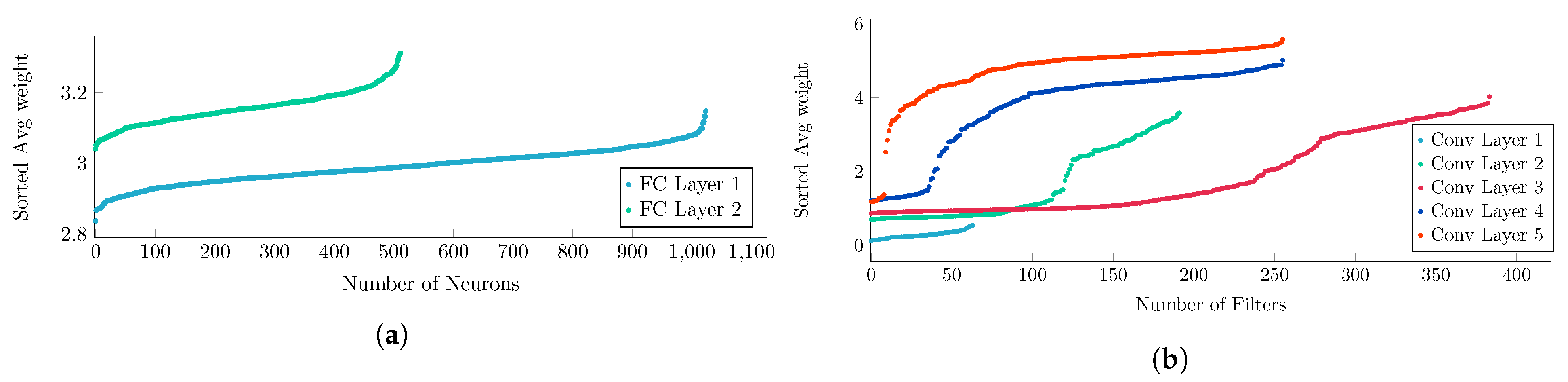
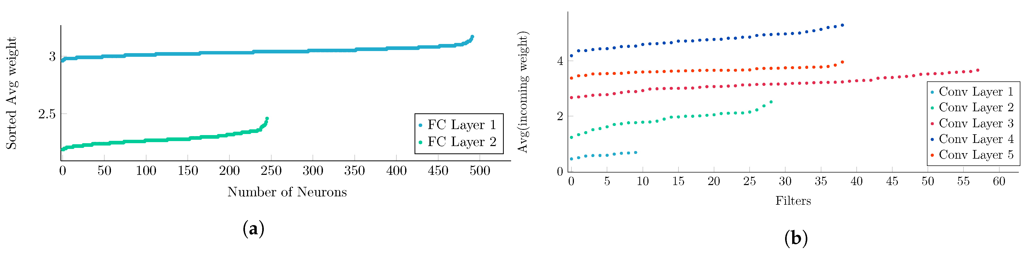
Using the presented pruning method, we were able to reduce the memory requirement of the models. A comparison of the pruned and original learnable model parameters is shown in Table 5. A smaller number of parameters implies less computational overhead and smaller memory footprint. This is very important during the inference phase. The impact of reducing the redundant parameters can be realized from the sorted average weights of the layers in Figure 9a,b.
After pruning the layers, the average weights are illustrated in Figure 9a and Figure 9b for two FC layers of the Autoencoder and five convolutional layers of AlexNet respectively. The layers used in Figure 5 and Figure 9 are the same except for the fact that the former are from the original model and later from the pruned model. Changes in the number of neurons and average weights result from the changed layer structure after pruning.
The sorted average weights have a flatter distribution after pruning compared to the weights in the original model. This justifies that after pruning the models, the remaining neurons contribute equally to the decision making for the current layer, while reducing the memory requirement.
Whether a model is suitable for the given inference task, does however depend on its accuracy. Therefore, there is a trade off between size reduction and achievable accuracy. The maximum accuracy difference between the pruned models and the original models is 3 % . An aggressive structured pruning is used in this work which is inference friendly for its dense matrix operations. But this poses a disadvantage of steep degradation in accuracy if no threshold is used. We chose a 3% threshold in this work. This explains the maximum accuracy loss, since the method ensures a minimal model size while staying within the threshold. Whether 3% are too much loss, is application specific and the threshold needs to be tuned for each scenario.
The confusion matrix from the original and pruned model predictions are shown in Figure 10 for LeNet. We chose to highlight the confusion matrix only for one model with CWT features, the results are however similar for all other combinations. There are three different types of bearing usage and each type has five bearing defects. In the figures showing confusion matrix, the three columns represent the three different bearing usage types. The first row of sub figures in Figure 10 are the results from the original models while the second row of confusion matrices are from pruned models for the same features.
In some cases individual classes might show an accuracy difference higher than 3 % compared to the original model. The average accuracy difference of the pruned models are not higher than 3 % when compared to average accuracy of the original model. This can be verified from Table 6, which also shows the accuracy of all combinations under test. It should be noted that the accuracy difference threshold ( 3 % in this work) is a sensitive parameter and depending on the application it can be bigger or smaller. A bigger threshold margin increases the chance to reduce the memory footprint of the model. We selected this threshold arbitrarily to demonstrate the pruning bottleneck in the work. For real applications, this threshold can be different for various applications and datasets.
Table 7 shows the inference time for AE and AlexNet model. Three different features STFT, CWT and 2D Time Signal were selected for this comparison as all of them have same dimensions. The model size corresponding to these features provides a bigger spectrum of analysis. While the STFT feature corresponds to one of the smallest models, CWT and 2D Time Signal correspond to models with more parameters. As already discussed in Section 3.4, the models were deployed on two different MCUs. Here, only the inference time on Nucleo H743Z2 is shown as the available flash memory suits the memory requirement of all the selected models. From the inference results, it is evident that XCubeAI is faster in comparison to TF Lite. As the MCU does not have a neural network accelerator hence the better performance in fast calculation can only be justified by a better software framework implementation from STM for XCubeAI. The inference time comparisons are consistent with the model size or the number of parameters for the TF Lite framework. On the other hand XCubeAI has ≈ 3 m s inference time for models with ≈3k, ≈75k and with ≈95k parameters.
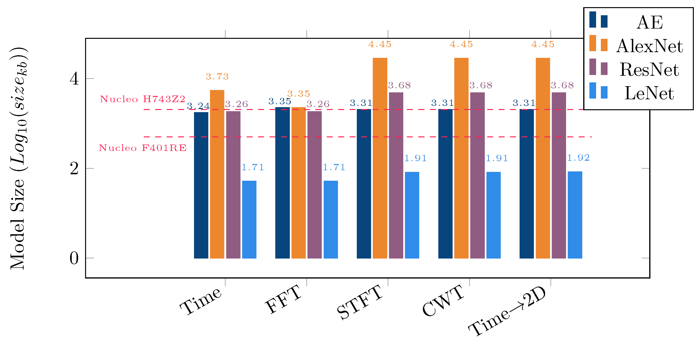
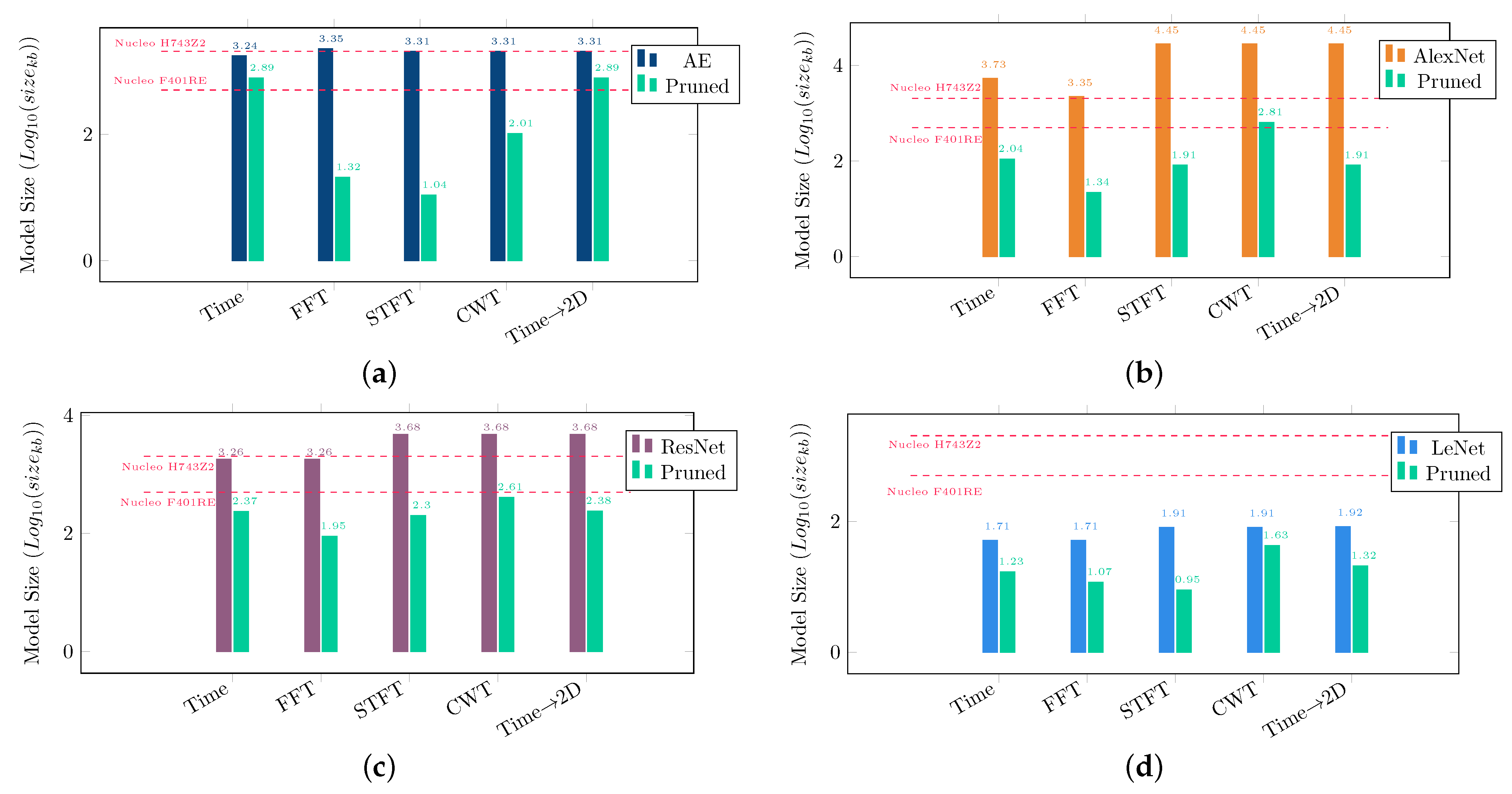
Figure 11a–d show the size comparison between the original model and the pruned model for different feature sets. This shows that most of the pruned models fit in both STM32 MCUs discussed in this work irrespective of the features used. However, there are differences in the resulting size depending on the choice of combination of feature and model. Clearly, spectral features (STFT and FFT) are the best choice for bearing classification. All the different types of model require less parameters to train on the spectral features. It is though interesting to observe that all the CNN models (AlexNet, ResNet, LeNet) use more parameters to train on CWT. On the other hand, 2D Time Signals needs less parameters to train on the same models. Although there have been many instances of application of Wavelet transforms (DWT) [36] for bearing fault detection but authors in this work have avoided to change the features compared to the benchmark study. It would interesting to investigate this in our future work though. The DWT implementation on arm MCUs are more energy efficient in comparison to the CWT implementation.
Regardless of features convolutional neural networks like AlexNet, ResNet and LeNet all perform quite well in bearing defect classification. Due to the smaller design and less number of layers in the LeNet model it is considered to be the most energy efficient and inference friendly. But the same design finds learning the CWT features problematic where the model achieves only ≈78% accuracy. Authors can only justify by understanding that the CWT feature needs deeper models like ResNet with ≈90% accuracy. ResNet model being the deepest of all, with highest number of parameters achieves best accuracy but requires larger memory and more flops while inferencing.
It should be noted, that the models which do not fit on the MCU is not because of a direct shortcoming of the pruning framework. This is rather the size we achieved when applying the accuracy vs memory footprint trade off with an accuracy difference threshold. In case of more sensitive applications where accuracy loss is unaffordable, other pruning approaches should be used.
In this work, we have not focused on a comparison of the available pruning approaches but rather on enabling inferencing the model on the edge for Pdm applications. Hence, we have not explored other ideas in order to reduce the memory footprint while keeping the model accuracy as it is. The results show, that there is further potential in testing different options to reduce the memory footprint.
In addition to the model memory footprint, other code will have to be executed. When inferencing our deployed models, we used a test dataset suitable to the model but the features were not extracted on the edge. The models which do fit into the memory but with a very slight margin cannot be considered a 100 % success because the data acquisition and feature extraction has to be done on edge as well and thus will add further code overhead.

5. Discussion

The goal of this work was to bring DNN based decision making models for predictive maintenance on low power MCUs which is demonstrated successfully in the results. This is helpful in optimized replacement strategies of bearings and avoiding sudden shut down in industrial appliances. Enabling the execution on the MCU comes at the cost of some compromise in accuracy. There is a trade off between model size and accuracy. The threshold of 3 % loss in accuracy between the original and the pruned model was decided before training and pruning the models. If the loss in accuracy is not feasible, decreasing the pruning percentage would also decrease the accuracy loss but will lead to bigger models as in our study. Hence there is a constrained bottleneck but our analysis on the weight distribution of fully connected and convolutional layers gives us new insights on further pruning strategies.
A pruning requirement for more sensitive industrial application cannot be neglected where margin of compromise of accuracy will be minimum or almost zero. In such cases, the pruning of the model becomes a strict constrained optimization problem. The discussion in Section 3.3 portrays optimization of only nodes or filters in detail which is one DNN hyperparameter as the pruning framework in [4] works only on trimming the network based on weights. But there can be several more approaches in optimizing the hyperparameters of the network which are unexplored for pruning the predictive maintenance models. This can be help in achieving the goal even with less loss in accuracy between the original and the pruned model.
The actual deployment of the model on MCU moves the theoretical perspective to a more pragmatic point of view. The deployment and inferencing of DNN models on MCU is a key novelty of this work. Clearly, as discussed in Section 4 XCubeAI inferences the DNN models faster as compared to TF Lite. But this has a vendor constraint. In order to deploy model with XCubeAI, only MCUs from STM must be used as of now as it does not support MCU from other vendors. But it should be understood that inference time is a very application dependent parameter. In a scenario of object tracking or detection on MCU, inference time is of utmost importance. On the other hand, in industrial scenarios where measurements are sometimes collected once or twice in a day an inference time of 40 s or even 1 min will not be a problematic parameter. In addition to this, we understand that more parameters imply a higher number of flops which inherently implies more clock cycles and larger inference time. Therefore, an important concern can be raised about energy consumption for all models implemented with XCubeAI with network parameters up to ≈95k. As the scope of the work does not include energy benchmarking based on the inference time, we will address this in our future work.
Our work focused on the deployment of DNN models on arm based MCUs with two STM MCUs as example. Further hardware such as MCUs from different vendors will be tested in the future. We did not consider specialized signal processing hardware such as Digital Signal Processors (DSPs) or Field Programmable Gate Arrays (FPGAs). DSPs and FPGAs can accelerate the execution of models thanks to specialized blocks. However, this kind of hardware can be programmed and tuned quite flexibly. Thus, this requires specific development to utilize the specific capabilities. Our method is however applicable to other hardware as well, because the pruning is the first step to fit the model into the memory which is then followed by a hardware dependent implementation. Therefore, the results will differ depending on the used toolchain, as e.g., XCubeAI gives specific optimized results for STM MCUs only.

6. Conclusions

In this paper, we investigated whether state of the art benchmark DNN models could be run on general purpose MCUs. Our study showed that this is not possible in most cases and that the model size needs to be reduced in order to enable the deployment. We then showed how such a reduction can be performed using a pruning framework. While this showed promising results, the reduction was not sufficient in some cases. As a final step, we deployed the models on the MCU in order to measure the inference time. The deployment brings together the theoretical approaches for model tuning and compression for predictive maintenance applications.
As a next step, we will analyze different pruning approaches to further reduce the model size while achieving higher model accuracy. Quantization methods will be added to a follow up comparison as well. The testing of the pruned models can be done with feature extraction on edge in order to consider the code overhead involved in the inferencing phase. Further investigations are needed to estimate the energy consumption during inference and to enhance the performance on the MCUs. In addition, we plan to evaluate the method on further hardware to see generalization effects.

Author Contributions

Conceptualization, R.P., S.K. and S.U.; methodology, R.P.; software, R.P.; validation, R.P., S.K. and S.U.; formal analysis, R.P.; investigation, R.P. and S.U.; data curation, R.P.; writing—original draft preparation, R.P. and S.K.; writing—review and editing, R.P., S.K., T.H. and S.U.; visualization, R.P. and S.K.; supervision, S.K.; project administration, S.U.; funding acquisition, T.H. All authors have read and agreed to the published version of the manuscript.

Funding

This research was financed by IMMS with funds from the German state of Thüringen.

Data Availability Statement

Not applicable.

Conflicts of Interest

The authors declare no conflict of interest.

References

  1. Upadhyay, R.K.; Kumaraswamidhas, L.A.; Azam, M.S. Rolling element bearing failure analysis: A case study. Case Stud. Eng. Fail. Anal. 2013, 1, 15–17. [Google Scholar] [CrossRef] [Green Version]
  2. Zhao, Z.; Li, T.; Wu, J.; Sun, C.; Wang, S.; Yan, R.; Chen, X. Deep learning algorithms for rotating machinery intelligent diagnosis: An open source benchmark study. ISA Trans. 2020, 107, 224–255. [Google Scholar] [CrossRef]
  3. Wang, B.; Lei, Y.; Li, N.; Li, N. A hybrid prognostics approach for estimating remaining useful life of rolling element bearings. IEEE Trans. Reliab. 2018, 69, 401–412. [Google Scholar] [CrossRef]
  4. Konegen, D.; Rüb, M. AutoFlow. 2021. Available online: https://github.com/Hahn-Schickard/AUTOflow (accessed on 20 December 2022).
  5. Abadi, M.; Agarwal, A.; Barham, P.; Brevdo, E.; Chen, Z.; Citro, C.; Corrado, G.S.; Davis, A.; Dean, J.; Devin, M.; et al. Tensorflow: Large-scale machine learning on heterogeneous distributed systems. arXiv 2016, arXiv:1603.04467. [Google Scholar]
  6. Shao, H.; Jiang, H.; Zhao, H.; Wang, F. A novel deep autoencoder feature learning method for rotating machinery fault diagnosis. Mech. Syst. Signal Process. 2017, 95, 187–204. [Google Scholar] [CrossRef]
  7. Saufi, S.R.; Ahmad, Z.A.B.; Leong, M.S.; Lim, M.H. Low-speed bearing fault diagnosis based on ArSSAE model using acoustic emission and vibration signals. IEEE Access 2019, 7, 46885–46897. [Google Scholar] [CrossRef]
  8. Chen, Z.; Li, W. Multisensor feature fusion for bearing fault diagnosis using sparse autoencoder and deep belief network. Trans. Instrum. Meas. 2017, 66, 1693–1702. [Google Scholar] [CrossRef]
  9. Li, X.; Jiang, H.; Zhao, K.; Wang, R. A deep transfer nonnegativity-constraint sparse autoencoder for rolling bearing fault diagnosis with few labeled data. IEEE Access 2019, 7, 91216–91224. [Google Scholar] [CrossRef]
  10. Shi, H.; Chen, J.; Si, J.; Zheng, C. Fault diagnosis of rolling bearings based on a residual dilated pyramid network and full convolutional denoising autoencoder. Sensors 2020, 20, 5734. [Google Scholar] [CrossRef]
  11. Xie, Y.; Zhang, T. Fault diagnosis for rotating machinery based on convolutional neural network and empirical mode decomposition. Shock Vib. 2017, 2017, 3084197. [Google Scholar] [CrossRef]
  12. Wen, L.; Li, X.; Gao, L.; Zhang, Y. A new convolutional neural network-based data-driven fault diagnosis method. IEEE Trans. Ind. Electron. 2017, 65, 5990–5998. [Google Scholar] [CrossRef]
  13. Pinedo-Sanchez, L.A.; Mercado-Ravell, D.A.; Carballo-Monsivais, C.A. Vibration analysis in bearings for failure prevention using CNN. J. Braz. Soc. Mech. Sci. Eng. 2020, 42, 628. [Google Scholar] [CrossRef]
  14. Xie, S.; Ren, G.; Zhu, J. Application of a new one-dimensional deep convolutional neural network for intelligent fault diagnosis of rolling bearings. Sci. Prog. 2020, 103, 0036850420951394. [Google Scholar] [CrossRef]
  15. Xu, W. Research on bearing fault diagnosis base on deep learning. In Proceedings of the 4th International Conference on Artificial Intelligence and Big Data (ICAIBD), Chengdu, China, 28–31 May 2021; pp. 261–264. [Google Scholar]
  16. Sharma, K.; Goyal, D.; Kanda, R. Intelligent Fault Diagnosis of Bearings based on Convolutional Neural Network using Infrared Thermography. Proc. Inst. Mech. Eng. Part J J. Eng. Tribol. 2022, 236, 2439–2446. [Google Scholar] [CrossRef]
  17. Wang, J.; Mo, Z.; Zhang, H.; Miao, Q. A deep learning method for bearing fault diagnosis based on time-frequency image. IEEE Access 2019, 7, 42373–42383. [Google Scholar] [CrossRef]
  18. Chen, Z.; Cen, J.; Xiong, J. Rolling bearing fault diagnosis using time-frequency analysis and deep transfer convolutional neural network. IEEE Access 2020, 8, 150248–150261. [Google Scholar] [CrossRef]
  19. Liang, P.; Wang, W.; Yuan, X.; Liu, S.; Zhang, L.; Cheng, Y. Intelligent fault diagnosis of rolling bearing based on wavelet transform and improved ResNet under noisy labels and environment. Eng. Appl. Artif. Intell. 2022, 115, 105269. [Google Scholar] [CrossRef]
  20. Peng, X.; Wang, Z.; Li, B.; Qian, L.; Jiao, B. Rolling Bearing Fault Diagnosis Based on PCA-ResNet. J. Phys. Conf. Ser. 2022, 2218, 012082. [Google Scholar] [CrossRef]
  21. Wang, C.; Xie, Y.; Zhang, D. Deep learning for bearing fault diagnosis under different working loads and non-fault location point. J. Low Freq. Noise Vib. Act. Control 2021, 40, 588–600. [Google Scholar] [CrossRef] [Green Version]
  22. Hao, X.; Zheng, Y.; Lu, L.; Pan, H. Research on Intelligent Fault Diagnosis of Rolling Bearing Based on Improved Deep Residual Network. Appl. Sci. 2021, 11, 10889. [Google Scholar] [CrossRef]
  23. Li, S.; Xie, G.; Ji, W.; Hei, X.; Chen, W. Fault Diagnosis of Rolling Bearing Based on Improved LeNet-5 CNN. In Proceedings of the 9th Data Driven Control and Learning Systems Conference (DDCLS), Liuzhou, China, 20–22 November 2020; pp. 117–122. [Google Scholar]
  24. Wan, L.; Chen, Y.; Li, H.; Li, C. Rolling-element bearing fault diagnosis using improved LeNet-5 network. Sensors 2020, 20, 1693. [Google Scholar] [CrossRef] [Green Version]
  25. Liu, N.; Ma, X.; Xu, Z.; Wang, Y.; Tang, J.; Ye, J. Autocompress: An automatic dnn structured pruning framework for ultra-high compression rates. In Proceedings of the AAAI Conference on Artificial Intelligence, New York, NY, USA, 7–12 February 2020; Volume 34, pp. 4876–4883. [Google Scholar] [CrossRef]
  26. Tang, Z.; Luo, L.; Xie, B.; Zhu, Y.; Zhao, R.; Bi, L.; Lu, C. Automatic Sparse Connectivity Learning for Neural Networks. IEEE Trans. Neural Netw. Learn. Syst. 2022, 1–15. [Google Scholar] [CrossRef]
  27. Li, Y.; Zhao, P.; Yuan, G.; Lin, X.; Wang, Y.; Chen, X. Pruning-as-Search: Efficient Neural Architecture Search via Channel Pruning and Structural Reparameterization. arXiv 2022, arXiv:2206.01198. [Google Scholar]
  28. Liu, Z.; Cheng, K.T.; Huang, D.; Xing, E.P.; Shen, Z. Nonuniform-to-Uniform Quantization: Towards Accurate Quantization via Generalized Straight-Through Estimation. In Proceedings of the IEEE/CVF Conference on Computer Vision and Pattern Recognition, New Orleans, LA, USA, 18–24 June 2022; pp. 4942–4952. [Google Scholar]
  29. Park, E.; Yoo, S.; Vajda, P. Value-aware quantization for training and inference of neural networks. In Proceedings of the European Conference on Computer Vision (ECCV), Munich, Germany, 8–14 September 2018; pp. 580–595. [Google Scholar]
  30. Onus, U.; Uziel, S.; Hutschenreuther, T.; Krug, S. Trade-off between Spectral Feature Extractors for Machine Health Prognostics on Microcontrollers. In Proceedings of the 2022 IEEE 9th International Conference on Computational Intelligence and Virtual Environments for Measurement Systems and Applications (CIVEMSA), Chemnitz, Germany, 15–17 June 2022; pp. 1–6. [Google Scholar]
  31. Burrello, A.; Garofalo, A.; Bruschi, N.; Tagliavini, G.; Rossi, D.; Conti, F. Dory: Automatic end-to-end deployment of real-world dnns on low-cost iot mcus. IEEE Trans. Comput. 2021, 70, 1253–1268. [Google Scholar] [CrossRef]
  32. Krizhevsky, A.; Sutskever, I.; Hinton, G.E. Imagenet classification with deep convolutional neural networks. Commun. ACM 2017, 60, 84–90. [Google Scholar] [CrossRef] [Green Version]
  33. He, K.; Zhang, X.; Ren, S.; Sun, J. Deep residual learning for image recognition. In Proceedings of the Conference on Computer Vision and Pattern Recognition (CVPR), Las Vegas, NV, USA, 27–30 June 2016; pp. 770–778. [Google Scholar]
  34. David, R.; Duke, J.; Jain, A.; Janapa Reddi, V.; Jeffries, N.; Li, J.; Kreeger, N.; Nappier, I.; Natraj, M.; Wang, T.; et al. Tensorflow lite micro: Embedded machine learning for tinyml systems. Proc. Mach. Learn. Syst. 2021, 3, 800–811. [Google Scholar]
  35. Microelectronics, S. X-CUBE-AI—AI Expansion Pack for STM32CubeMX. 2017. Available online: https://www.st.com/en/embedded-software/x-cube-ai.html (accessed on 20 December 2022).
  36. Patil, A.B.; Gaikwad, J.A.; Kulkarni, J.V. Bearing fault diagnosis using discrete Wavelet Transform and Artificial Neural Network. In Proceedings of the 2016 2nd International Conference on Applied and Theoretical Computing and Communication Technology (iCATccT), Bengaluru, India, 21–23 July 2016; pp. 399–405. [Google Scholar] [CrossRef]
Figure 1. Vibration signals acquired for a complete run to failure of a bearing.
Electronics 12 00639 g001
Figure 2. Illustration of convolutional and pooling operation in respective layers. (a) Convolution operation in CNN; (b) Average and Max pooling operation in CNN.
Electronics 12 00639 g002
Figure 4. Block Diagram of CNN models.
Electronics 12 00639 g004
Figure 5. Analysis of sorted weights for FC and convolutional layers from AE and AlexNet model respectively. (a) Sorted Avg weights from two FC layers of AE model; (b) Sorted Avg weights from five convolutional layers of AlexNet model.
Electronics 12 00639 g005
Figure 6. Possible permutations of layers after a convolutional layer.
Electronics 12 00639 g006
Figure 7. Flow chart for the pruning algorithm.
Electronics 12 00639 g007
Figure 8. Comparison of required memory size of AE, AlexNet, ResNet and LeNet for different feature sets.
Electronics 12 00639 g008
Figure 9. Analysis of sorted weights for FC and convolutional layers from pruned AE and AlexNet model respectively after retraining. (a) Sorted average weights from two FC layers from pruned AE model; (b) Weights from five convolutional layers from pruned AlexNet model.
Electronics 12 00639 g009
Figure 10. The figure represents confusion matrix for LeNet model with CWT features. We have three types of bearing load conditions with each condition having five defects. Three columns represent three bearing load conditions. The first and second row represent prediction results from original and pruned LeNet model respectively.
Electronics 12 00639 g010
Figure 11. Comparison of size of AE, AlexNet, ResNet and LeNet for different feature sets with pruned model sizes. (a) Comparison of model size between benchmark and pruned AE model for different features; (b) Comparison of model size between benchmark and pruned AlexNet model for different features; (c) Comparison of model size between benchmark and pruned ResNet model for different features; (d) Comparison of model size between bench mark and pruned LeNet model for different features.
Electronics 12 00639 g011
Table 1. Comparison among the State Of The Art works and the current work.
SOTABearing DiagnosticsML/DNNModel CompressionDeployment
[9]SAE
[21]ResNet
[17]AlexNet
[30]Spectral Features✗ (Theoretical)
[26,27]ResNet
[25]ResNet✓ (Smartphone)
[31]DNNs✓ (PULP)
[28,29]ResNet
ThisResNet, AlexNet, AE✓ (MCU)
Table 2. Structural details for the AE, SAE and DAE models. As SAE and DAE are structurally similar to AE only details for AE are mentioned.
Autoencoder (1D)Autoencoder (2D)
LayersParametersLayersParameters
Input 512 × 1 or 1024 × 1 Input 32 × 32 × 1
FC 1 + Batch NormUnits: 1024 or 512Conv 1 + Batch Normkernel: 3 × 3 , Filters: 3
FC 2 + Batch NormUnits: u p r e / 2 Conv 2 + Batch Normkernel: 3 × 3 , Filters: 32
FC 3 + Batch NormUnits: u p r e / 2 Conv 3 + Batch Normkernel: 3 × 3 , Filters: 32
FC 4 + Batch NormUnits: u p r e / 2 Conv 4 + Batch Normkernel: 3 × 3 , Filters: 32
FC 5 + Batch NormUnits: u p r e / 2
FC 6Units: 64FC 1Units: 256
FC 6Units: 16FC 2Units: 16
Output15 classesOutput15 classes
W l e a r n 1,755,983 W l e a r n 2,120,915
Table 3. Structural details of AlexNet, ResNet and LeNet used in this work.
AlexNetResNetLeNet
LayersParametersLayersParametersLayersParameters
Input 32 × 32 × 1 or 1024 × 1 Input 32 × 32 × 1 or 1024 × 1 Input 32 × 32 × 1 or 1024 × 1
or 512 × 1 or 512 × 1 or 512 × 1
Conv 1kernel: 3 × 3 , Filters: 64Conv 1kernel: 7 × 7 , Filters: 64Conv 1kernel: 5 × 5 , Filters: 6
Conv 2kernel: 3 × 3 , Filters: 192Res Block 1: Conv(right)kernel: 3 × 3 , Filters: 64,64Conv 2kernel: 5 × 5 , Filters: 16
Conv 3kernel: 3 × 3 , Filters: 384Res Block 2: Conv(right)kernel: 3 × 3 , Filters: 128,128Conv 3kernel: 5 × 5 , Filters: 120
Conv 4kernel: 3 × 3 , Filters: 256Res Block 2: Conv(left)kernel: 1 × 1 , Filters: 128
Conv 5kernel: 3 × 3 , Filters: 384Res Block 3: Conv(right)kernel: 3 × 3 , Filters: 256,256
Res Block 3: Conv(left)kernel: 1 × 1 , Filters: 256
Res Block 4: Conv(right)kernel: 3 × 3 , Filters: 512,512
Res Block 4: Conv(left)kernel: 1 × 1 , Filters: 512
FC 1Units: 4096 FC 1Units: 120
FC 2Units: 4096 FC 2Units: 84
Output15 classesOutput15 classesOutput15 classes
W l e a r n 1,235,456 (1D) W l e a r n 1,235,456 (1D) W l e a r n 1,235,456 (1D)
1,235,456 (2D) 1,235,456 (2D) 1,235,456 (2D)
Table 4. Dataset and model training details.
(a) Dataset Description(b) Training parameters
FeaturesDescriptionTraining Details
Data SamplesDimensionParametersValues
Time domain signals1920 1024 × 1 Epochs100
FFT1920 512 × 1 Batch size64
STFT1920 32 × 32 OptimizerAdam
CWT1920 32 × 32 Learning rate0.001
2D Time Signals1920 32 × 32 Loss functionSparse Categorical Cross Entropy
Table 5. Comparison of learnable parameters in original and pruned model.
FeaturesAEAlexNetResNetLeNet
OriginalPrunedOriginalPrunedOriginalPrunedOriginalPruned
Time Signals1,755,983668,9805,511,63197,6731,761,679228,13736,2554995
FFT2,283,34311,7573,414,47998261,761,67987,90736,255927
CWT2,120,91595,32428,534,479656,6204,910,095415,39476,69534,120
2D Time Signals2,120,915798,93328,534,47975,6274,910,095244,52276,69512,887
STFT2,120,915249628,534,47975,6274,910,095205,24176,6951967
Table 6. Comparison of accuracy for original and pruned model.
FeaturesAEAlexNetResNetLeNet
OriginalPrunedOriginalPrunedOriginalPrunedOriginalPruned
Time Signals80.2%77.60%96.1%93.23%99.73%97.02%97%95.31%
FFT99.73%97.39%98.4%96.87%99.21%97.84%98.03%96.09%
CWT89.67%87.15%90.02%87.43%92.91%90.23%80.47%78.36%
2D Time Signals85.14%84.17%97.7%95.35%95.57%93.23%96.5%94.01%
STFT99.67%98.18%98.37%97.65%99.6%96.35%98.07%97.13%
Table 7. Comparison of Inference time for CWT, STFT and 2D time signal features for AlexNet and AE on Nucleo H743Z2.
ModelCWTSTFT2D Time Signal
XCubeAITF LiteXCubeAITF LiteXCubeAITF Lite
AE m s 8905  m s m s 135  m s 40  m s 39,775  m s
AlexNet34  m s 38,173  m s m s 5195  m s m s 5196  m s
Disclaimer/Publisher’s Note: The statements, opinions and data contained in all publications are solely those of the individual author(s) and contributor(s) and not of MDPI and/or the editor(s). MDPI and/or the editor(s) disclaim responsibility for any injury to people or property resulting from any ideas, methods, instructions or products referred to in the content.

