Article

TMD-BERT: A Transformer-Based Model for Transportation Mode Detection

by
Ifigenia Drosouli
1,2,
Athanasios Voulodimos
3,*,
Paris Mastorocostas
1,
Georgios Miaoulis
1 and
Djamchid Ghazanfarpour
2
1
Department of Informatica and Computer Engineering, University of West Attica, 12243 Egaleo, Greece
2
Department of Informatics, University of Limoges, 87032 Limoges, France
3
School of Electrical and Computer Engineering, National Technical University of Athens, 15773 Athens, Greece
*
Author to whom correspondence should be addressed.
Electronics 2023, 12(3), 581; https://doi.org/10.3390/electronics12030581
Submission received: 11 December 2022 / Revised: 13 January 2023 / Accepted: 19 January 2023 / Published: 24 January 2023
(This article belongs to the Special Issue Deep Learning for Computer Vision and Pattern Recognition)

Abstract

:
Aiming to differentiate various transportation modes and detect the means of transport an individual uses, is the focal point of transportation mode detection, one of the problems in the field of intelligent transport which receives the attention of researchers because of its interesting and useful applications. In this paper, we present TMD-BERT, a transformer-based model for transportation mode detection based on sensor data. The proposed transformer-based approach processes the entire sequence of data, understand the importance of each part of the input sequence and assigns weights accordingly, using attention mechanisms, to learn global dependencies in the sequence. The experimental evaluation shows the high performance of the model compared to the state of the art, demonstrating a prediction accuracy of 98.8%.

1. Introduction

Transportation, nowadays, is an important factor influencing urban areas and has a promising role in the development of smart cities. Moving from one place to another is a major part of citizens’ life. Citizens are constantly moving and changing means of transport according to their needs, thus it may be of extensive research interest how transportation may evolve over time. Having knowledge of how individuals move at a given time but also predicting the way they may move in the future, can have useful benefits for city residents and authorities at many points of everyday life. Improving infrastructure, designing a city friendly to the citizen, planning a convenient transport system, providing targeted real-time information and updating according to personal needs, managing traffic congestion, protecting the environment by promoting soft transportation modes (cycling, running, and walking), enhancing the physical and mental health of citizens, are some of these benefits [1].
Transportation Mode Detection (TMD), frequently considered as a subfield of the field of human activity recognition [2,3,4], intends to differentiate various transportation modes and identify the means of transport an individual uses.
The progress of the Internet of things (IoT), big data, and cloud computing has completely revolutionized transportation. Modern mobile devices such as smartphones, tablets, smartwatches, etc., have given a huge boost and space for further development in the field of TMD by collecting and analyzing multimodal sensor data in the transportation area. The fact that these devices are outfitted with various sensors, such as accelerometer, gyroscope, hygrometer, magnetometer, sound, and image sensor, etc., allows them to provide precise, accurate, and ready to use, data. This fact, combined with the increasing [5] and continuous use of the mobile device in any form of humans mobility [6], makes it more possible than before to capture information that, until now, was inaccessible, such as where the individual is, what transport media the passengers prefer to use, the duration of their trip and even recognize their daily travel activity patterns [7].
At the same time, the prodigious advances in the Deep learning area, create new perspectives in the transport community, and in particular in smart mobility. Although deep learning models such as CNN and LSTM [8] have been applied to TMD yielding remarkable results, there are still certain limitations in such approaches, mainly pertaining to the handling of long-range dependencies. Transformers, an innovative deep learning implementation introduced in 2017 [9], address these limitations, as it is capable of learning relations between elements thanks to multi-head attention mechanisms and positional embeddings. Transformers analyze the entire sequence of data, understand the importance of each segment of the input sequence, and appropriately allocate weights by means of attention mechanisms, in order to learn global dependencies in the sequence and do not merely focus on adjacent events.
Transformers are extensively used in Natural Language Processing (NLP) field and later in other fields, too, such as computer vision, but to our knowledge, little research has been performed to investigate Transformers models application in the area of intelligent transport. This work assumes the smart device sensor values for each timestamp as sequences and each measurement as a word. We operate BERT (Bidirectional Encoder Representations from Transformers), an open-sourced, pre-trained model, in order to predict the transportation media an individual will use at a specific time in the future, using the media we know that has been used in the recent past. The remainder of the paper is structured as follows: In Section 2 there is a brief overview of related work, while in Section 3 the proposed transformer-based TMD-BERT model is presented. Section 4, offers an extensive experimental evaluation of the proposed model in comparison with traditional deep learning methods. Finally, Section 5 concludes the paper with a summary of our findings.

2. Related Work

This section presents an analysis of existing research partitioned into two sections, namely research on deep learning in TMD and a brief overview of research on applications of transformers.

2.1. Research on Deep Learning in TMD

During the last few years, traditional Machine Learning as well as Deep Learning techniques have been used to develop several models based on sensors embedded in smartphones, (magnetometer, accelerometer, gyroscope, atmospheric pressure, GPS, etc.), with the aim of determining the mode of transportation used by a citizen. In [10], a number of traditional Machine Learning models, such as Decision Trees, Random Forests, Multi-Layer Perceptrons, and Support Vector Machines, to classify five actions (bus, train, walking, still, car), applied on a sensor-based dataset they created. The experiments resulted in an accuracy of 81–93% achieved by Random Forest. In [11], several Machine and Deep Learning techniques for detecting transportation modes in real-time, have been presented, using and comparing extracted statistical features and raw data as input. Recurrent Neural Networks (RNN) achieved 88% accuracy by using statistical features whereas Convolutional Neural Networks (CNN) achieved 98.6% accuracy without any pre-processing of raw data measurements. A CNN model built on acceleration data was used in [12] to recognize the transportation mode an individual uses when moving. This model compared with a variety of ML and DL classification models (decision trees, k-nearest neighbors algorithm, naïve Bayes, adaptive boosting, support vector machines, shallow neural network, and long short-term memory networks) achieved an accuracy of 94.48% [13]. Instead of raw data, a novel set of time and frequency extracted features were used to apply an LSTM model and recognize 10 media of transport with an accuracy of 96.82%.

2.2. Research on Transformers

Transformers [9] adopt an attention mechanism which examines an input sequence and decides at each step the importance of the other parts of the sequence. Since their introduction, they have been gradually shown to outperform LSTM which was the previous state-of-the-art model in sequential data analysis. Attention was initially designed in the context of Neural Machine Translation using Seq2Seq Models in the Natural Language Processing (NLP) field. In NLP, both attention mechanism and transformers have been used effectively in a variety of tasks such as reading comprehension, abstractive summarization, word completion, and others [14,15,16].
Before Transformers appeared, most state-of-the-art NLP models were based on RNN [17], LSTM [18], or CNN [19], however, these methods presented certain limitations. RNN [20,21] processed data sequentially but firstly this was not very efficient in handling long sequences and secondly, it was difficult to take full advantage of modern fast computing devices such as TPUs and GPUs. Even though LSTM offered a slight improvement over conventional RNN concerning long dependency issues, there were still particular constraints such as the need for sequential processing that not allowed parallel training and the difficulty in handling long sequences and long-range dependencies. Convolutional Neural Networks (CNNs) [22], widely used in the NLP field, trained quite fast and were efficient with short texts, but the number of different kernels required to capture dependencies between all possible combinations of words in a sentence, would be huge and impractical. On the other hand, the reason Transformers outperform all other architectures is the fact that they completely avoid recursion. That is because, thanks to multi-head attention mechanisms and positional embeddings, they process sentences as a whole and they learn relationships between words.

3. The Transformer Model for Transportation Mode Detection

The additional feature of training parallelization allows training on larger datasets than was once possible. This feature led to the development of pre-trained systems such as BERT (Bidirectional Encoder Representations from Transformers) [23] which was trained with large language datasets, such as the Wikipedia Corpus and Common Crawl. Thus, although Transformers were used primarily in the fields of natural language processing (NLP), the development of pre-trained systems such as BERT sparked a wave of research in other domains, too. In the Computer Vision domain, models which can be well adapted to different image processing tasks were developed. In [24], ImageGPT a sequence Transformer is trained to auto-regressively predict pixels, without built-in knowledge of the 2D input structure. In [25], a pre-trained model with transformer architecture is developed for image processing, and in [26], Facebook AI researchers presented DETR showing that transformers can be used for object detection and segmentation, with very competitive results. In Biology and Chemistry research field, the AlphaFold2 model [27] was developed, an equivariant structure prediction module for protein structure prediction, as well as SE(3)-Transformers [28] a variant of the self-attention feature for 3D point clouds and graphs, which is equivalent under continuous 3D rotational translations. In the Transportation domain, spatial transformer [29], a new variant of graph neural networks has been developed. This model uses directed spatial dependencies with a self-attention mechanism and manages to capture and predict traffic flows in real time. In [30] TrafficBERT is proposed, a model for traffic flow prediction which is based on pre-trained BERT and can be used on a variety of roads as it is pre-trained with a large traffic dataset.
The goal of this paper is to build a robust and optimized TMD system that accepts a sequence of information from multiple smartphone sensors as input, and produces a prediction output of increased detection and prediction accuracy compared to existing traditional recurrent networks. The proposed TMD-BERT model leverages the representational power and other strengths of the transformer network family. It processes the entire sequence of data and learns global dependencies in the sequence, and provides a robust and accurate approach for TMD that outperforms existing methods, as shown in the experimental evaluation.

3.1. Transformer Models Overview

The basic transformer network model comprises a multi-head attention module and a position-wise feed-forward network. The normalized input sequence enters i the multi-head attention layer, which computes attention scores. These are then passed on to a position-wise feed-forward layer.
Attention mechanism in transformers is affected as a Query-Key-Value (QKV) model. Attention is composed of a series of linear transformations which analyze input sequences in an order-invariant fashion, calculating and allocating importance weights to each spot in the sequence. Single-head dot-product attention mechanism therefore applies linear transformations to the input signal to form query (Q), key (K) and value (V) matrices. Let us assume that x s b × s l is the input sequence, where s b is the batch size and s l the input length of (normalized and preprocessed) transportation-related sensor feature data (see details in following sections). Then the linear transformations can be represented by the matrices: W q s l × s q , W k s l × s k and W v s l × s v . Then Q = W q T x ,     K = W k T x ,     V = W v T x . Allowing weight matrices to have the same dimensions for easier matrix computations, s q = s k = s v , the single-head dot product attention A is a matrix multiplication of Q, K and V following a scaling and softmax operation.
A ( Q ,   K ,   V ) = s o f t m a x ( Q K T s k ) V
The first term in the above equation can be seen as the weighting of values at all locations of the sequence. Attention thus can inherently comprehend which parts of the sequence are significant to estimate the output and overlook parts that are not significant. This attribute is especially useful in the cases of imbalanced datasets since the respective weight for negative samples can automatically be set to a small value.
Further, transformers deploy a multi-head attention mechanism, rather than simply applying a single attention function. Multi-Head Attention is computed by extending the single-head attention mechanism to h dimensions (multiple heads) by appending the single-head attention outputs, followed by a linear layer.
M u l t i H e a d   A t t e n t i o n = C o n c a t   ( A ( Q i , K i ,   V i ) ) ,   i = 1 , ,   h
The normalized attention scores are then fed to a position-wise feed-forward layer (PFFN) that performs linear transformations with Gaussian Error Linear Units (GELU) activation function. The linear transformations are applied to each position individually and identically; in other words, the transformations utilize the same parameters for all positions of a sequence and differentiated parameters across layers. Denoting the attention sub-block output as a and the weight matrices and bias vectors of the linear transformations as W 1 ,   b 1 and W 2 ,   b 2 respectively yields:
P F F N ( a ) = G E L U ( 0 ,   a W 1 + b 1 ) W 2 + b 2

3.2. TMD-BERT Model

In this work, we used BERT to train a text classifier and built a model that was fine-tuned on our data in order to produce a state-of-the-art predictions. Specifically, an untrained layer of neurons was added to the end of the pre-trained BERT model and then the new model was trained for our classification task. The selection of a pre-trained model rather than developing a specific deep learning model (LSTM, CNN, etc.) that is suitable for the specific task is justified by the fact that developing such complex models requires high-performance computing resources so by using a pre-trained model as base, it makes possible to develop high-performance models and solve complicated problems efficiently.
An overview of TMD-BERT model is presented in Figure 1. More specifically, the implementation of the model consisted of four phases.
I. Time data from sensors: the dataset, a series of time data sensors, was already a supervised learning problem with input and output variables. II. Data Preprocessing: The data preparation process included (a) Resampling so that the data would be available at the same frequency that we wanted to make predictions, (b) downsampling in order to decrease the frequency of the samples from milliseconds to minutes and (c) normalization, by rescaling real-valued numeric attributes into a 0 to 1 range to make model training less sensitive to the scale of features. The goal was to establish a multivariate prediction model so that multiple, recent timesteps could be used to make the prediction for the next timestep. The preprocessing phase was completed in two schemas, one with and one without Dimensionality Reduction with Principal Component Analysis (PCA), in order to investigate its effect on the model performance. III. Bert model: Because the labels were imbalanced, we split the data set using for each class 85% for training and 15% for testing. The inputs were tokenized using BERT tokenizer by instantiating a pre-trained BERT model configuration to encode the train and test data. IV. Prediction: An output of increased detection and prediction accuracy was predicted.
In more detail, the maximum length of the sentences was 256. There are many variants of pre-trained BERT models. In this work, bert-base-uncased was used. The BERTBase model uses 12 layers of transformers block with 768-hidden layers, 12 self-attention heads, and around 110M trainable parameters. It is trained on lower-cased English text. We used BERT architecture with also adding a linear layer for predicting the output. The last hidden layer which corresponds to the [CLS] token was imported to the output layer of size num_classes which is eight here. Hence, we set the flag do_lower_case to true in BertTokenizer. The input to the BERT model was the set of measurements for each timestamp that was treated as a sequence so that one sequence would be classified as one of the eight labels. BertForSequenceClassification is the Bert Model transformer with a sequence classification/regression head on top (a linear layer on top of the pooled output). The model was tested for various batch sizes and the different number of epochs so as to avoid any possible underfitting and improve the overall model performance. One epoch was finally chosen among several numbers of epochs tested, as there was no significant performance improvement in comparison with timely execution. We used batch size 1 as a larger batch size resulted in CPU memory overflow. We used a Random sampler just for the training set, so that the model is more representative of the overall data distribution. For the validation set, balancing batches is not an issue, so a sequential sampler was used. We also used the Adam optimizer, which is “computationally efficient, has little memory requirement, invariant to diagonal rescaling of gradients, and is well suited for problems that are large in terms of data/parameters” [31]. The learning rate was initially set to 0.00001 and epsilon is a very small number to prevent any division by zero in the implementation. Get_linear_scheduler_with_warmup creates a schedule with a learning rate that after a warmup period during which it increases linearly from 0 to the learning rate set in the optimizer, it then starts to decrease linearly to 0. The hyper-parameters of the model are summarized in Table 1.
For the reason that BERT requires inputs in a specific format, for each tokenized input sentence, there were created:
  • Input ids which are a sequence of integers that represent each input token in the vocabulary of BERT tokenizer.
  • Attention mask which is a sequence of 0 for padding and 1 for input tokens.
  • Labels which are a sequence of 0 and 1 that represent the 8 labels of transportation modes.
In Figure 2 the fine-tuning procedure for sequence classification tasks is visualized. The final hidden state of the [CLS] token which is taken as the input sequence, is imported to the classification layer. That has a dimension of 8 (number of labels) × H (size of the hidden state). In the figure, E represents the input embedding, Ti represents the contextual representation of token I, and [CLS] is a special symbol that represents the classification output.
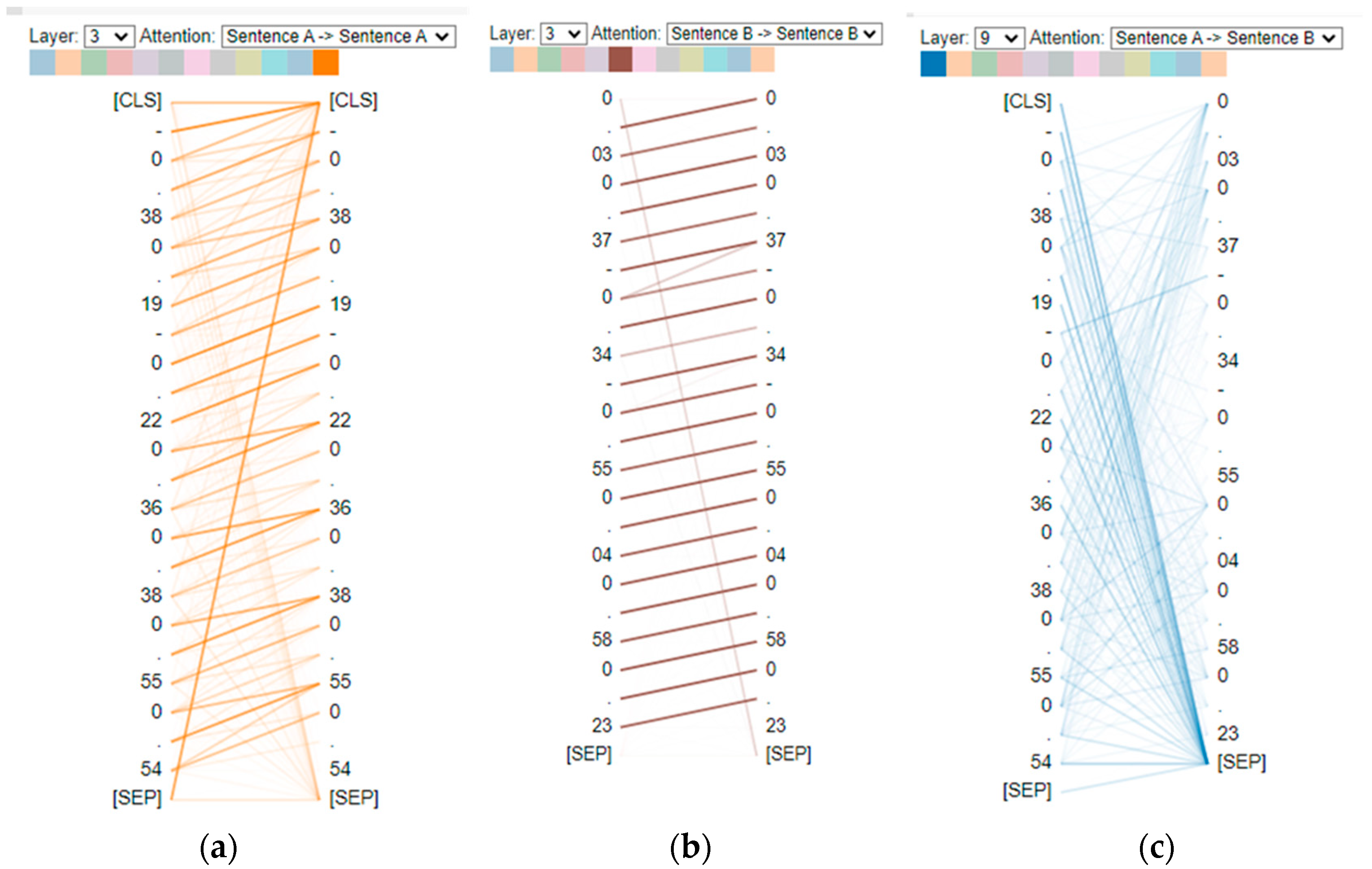
As mentioned before, the attention mechanism allows the model to comprehend the relation between words taking into consideration the content of the sentence. Attention provides us with a way in which we can see how BERT forms complex representations to understand language. Using BertViz [32], an interactive tool developed to visualize attention in BERT from multiple perspectives, Figure 3 depicts the attention resulting from an input text from our dataset, “−0.38 0.19 −0.22 0.36 0.38 0.55 0.54” and “0.03 0.37 −0.34 −0.55 0.04 0.58 0.23”, with the values representing the seven PCA principal components on particular timestamps. Self-attention is represented by colored lines depending on the color that corresponds to each attention head. These lines connect the tokens that are attending (left) with the tokens being attended to (right). The line weight reflects the attention score. For example, in Figure 3, for different layers and attention heads, in (a) each word seems to attend to more than one previous word with attention distributed in a slightly uneven way across previous words in the sentence. In contrast, in (b) each word seems to attend strongly to the immediately preceding word in the sentence. Finally, in (c) there is a between-sentence connection without a specific pattern for this sentences case. The fact that the attention head focuses on the [SEP] token indicates that it cannot find anything else in the input sentence to focus on.
The above visualizations show a mechanism of attention within the model, but BERT learns multiple mechanisms of attention, i.e., heads, that operate alongside with each other. In contrast with single-attention-mechanism, multi-head attention has the benefit that the model can capture a more extensive range of word relations. Figure 4 shows the attention in all the heads at once time for the same input text as before (i.e., “−0.38 0.19 −0.22 0.36 0.38 0.55 0.54” and “0.03 0.37 −0.34 −0.55 0.04 0.58 0.23”). Each cell shows the attention pattern for a specific head (column) in a particular layer (row). From this visualization, we can see that BERT produces a rich array of attention patterns.

4. Experimental Evaluation

In this section, the performance analysis of the proposed TMD-BERT model is presented. At first, there is a brief description of the dataset, then the data preparation is presented and finally, the analysis of the results follows.

4.1. Dataset Description

The dataset exploited in the experiments of this work, is a part of the initial Sussex-Huawei Locomotion-Transportation (SHL) dataset. It comprises 68 days of recording during a period from 1 March 2017 to 5 July 2017 and it was collected from one participant’s phone sensors. The phone was in his trouser’s front pocket. The participant used a variety of 8 transportation modes: Still, Walk, Run, Bike, Car, Bus, Train, and Subway. The measurements are derived from four smartphone sensors: magnetometer, accelerometer, gyroscope, and pressure sensor, which measure temperature, pressure, and altitude. The data set consists of 181,319 timestamps. The goal was to frame a forecasting problem for predicting the transportation mode that will be used at the next timestep, given the sensor measurements and transportation mode used in past, and recent timesteps.

4.2. Preliminary Data Analysis

The dataset used in the experiments was a supervised learning problem that had input and output variables (labels). The feature values per class are shown in Table 2.
The fact that one certain class categories comprise a larger proportion of the dataset than others, is not an issue in this work firstly because none of the transportation modes is more significant than others, secondly Bert seems to handle imbalanced classification well, thus removing the need to use standard data augmentation methods so as to limit this problem of imbalance [33] and thirdly, as it appears from the results all classes are predicted regardless of the samples number for each class.
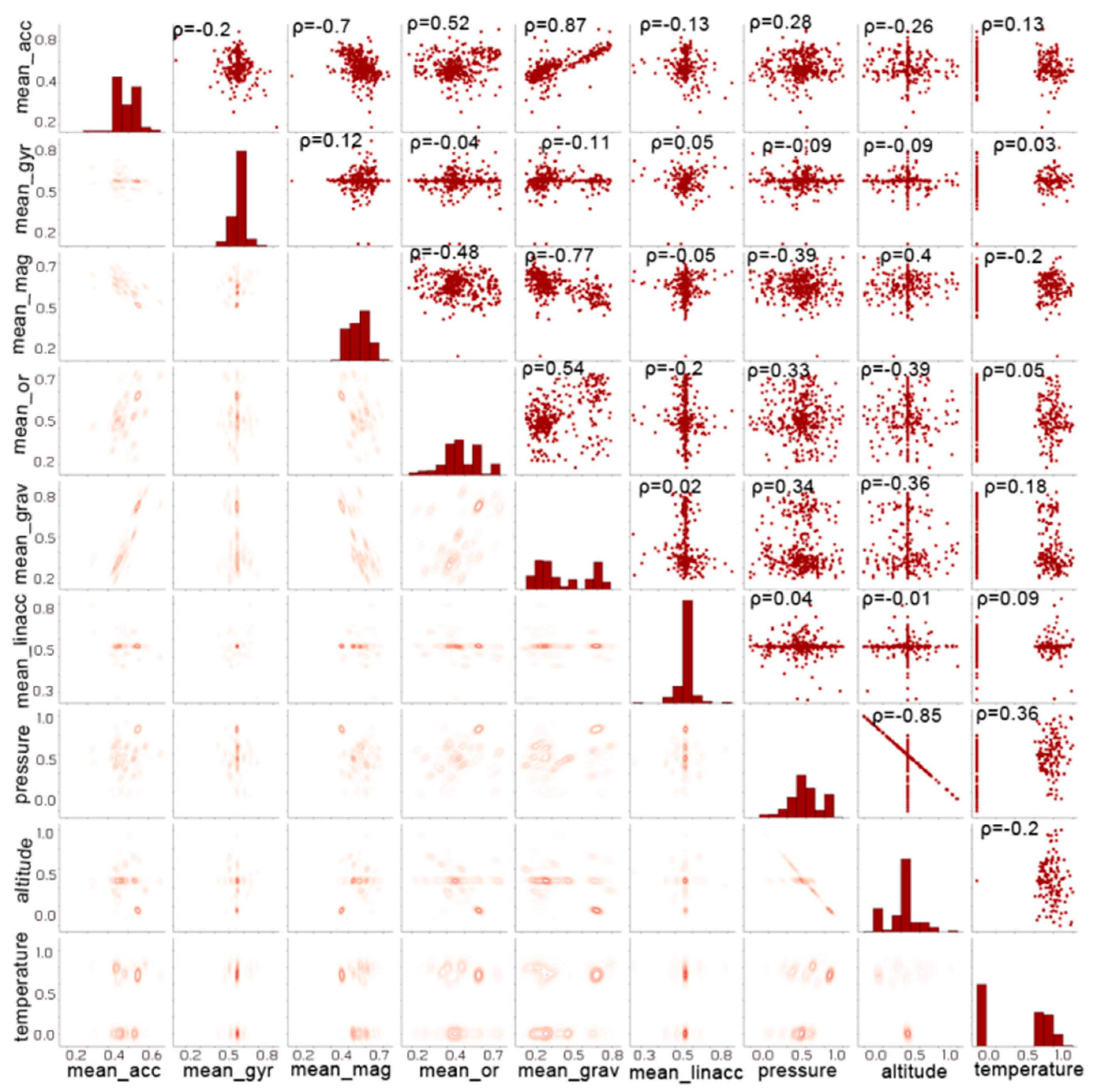
Figure 5 shows the distribution of all sensor measurements, including the mean value of the 3 or 4 axes of acceleration, magnitude, orientation, gravity and linear acceleration, as long as the temperature, pressure, and altitude values. The same features were used to calculate correlation in pairs.
The results of the correlation analysis were calculated using Pearson’s Correlation Coefficient (PCC) [34] and are shown in Figure 6. The PCC appears above the scatterplot for every pair of features. It shows the linear relationship between two sets of data by returning a value of between −1 and +1. The highest positively correlated pairs of features are acceleration-gravity (ρ = 0.87) and the highest negative ones are altitude and pressure (ρ = −0.85), as long as gravity and magnitude (ρ = −0.77). Most of the other pairs of features have a low percentage of interaction. In order to additionally visualize the insights of the dataset, not only on the interrelationship between sensor parameters but on the single machine learning variable distribution, too, the diagonal of the pair plot diagram shows the distribution of every single variable whereas the lower triangle depicts the probability distribution of one with respect to the other values.

4.3. Data Preparation

The dataset, having input and output variables, was already a supervised learning problem. For better performance, data was processed by dropping rows with class 0 (null class) and by sorting time values by date. Taking into consideration the fact that switching between modes of transport can be quite frequent, the dataset was resampled at a 1-minute time-window frequency, by making a downsampling from milliseconds to minutes. The problem was framed so that recent time steps could be used to predict the transport mode for the next time step. Also, the input features were normalized because of the different scales in input values.
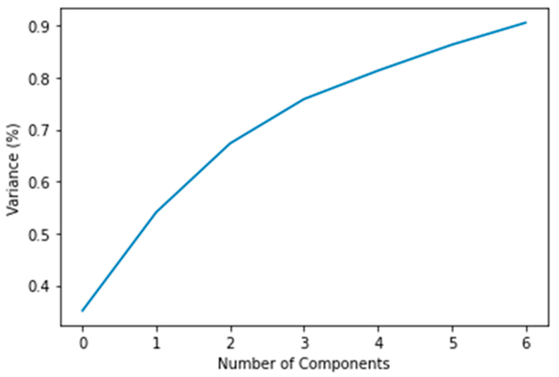
Two different approaches were tested before feeding the input data to the model. Firstly, the data was used as the initial set of 22 features. After that, before applying BERT, a dimensionality reduction algorithm was applied, so as to reduce the dimension of the training data and examine whether this will affect and to what extent the performance of the model. Because this study assumes the sensor values for each timestamp as sequences and each measurement as a word, the values were rounded to 2 decimal places so to have a more distinct and clear vocabulary. The technique used for dimensionality reduction was Principal Component Analysis (PCA). A number of n-components values were tested to fulfill the best model performance. As presented in Figure 7, in order to implement PCA, seven principal components were the best choice so as to keep over 90% of the total variance of the data.

4.4. Experimental Results

In this subsection, the performance of the proposed optimized BERT model is evaluated. As a benchmark to the BERT model in order to determine transportation modes, LSTM was used, since it is the best-performing model up to the present.
The LSTM model was defined as having 64 neurons in the first hidden layer, a Softmax activation function which is popularly used for multiclass classification problems, and 8 output values in the output layer. Categorical cross-entropy was used as a method to calculate errors and Adam optimizer with a learning rate of 0.001 in order to update the weights of the neural network. According to [31], Adam is “computationally efficient, has little memory requirement, and is well suited for problems that are large in terms of data/parameters”. Additionally, dropout was implemented to randomly drop 20% of units from the network. Various tests were performed on the number of epochs and batch sizes until the appropriate values were selected for optimal results in model performance. In summary, the LSTM model hyperparameters are presented in Table 3.
The performance evaluation of various classification models, was implemented by calculating several metrics, i.e., accuracy, precision, recall, F1-score, confusion matrix, Matthews correlation coefficient (MCC), and Cohen Kappa Score (CKS). Among these, the weighted F1-score was selected as the most representative metric, because it corresponds to the average F1-score value, taking into consideration the proportion of each class in the dataset. For forecasting, 1 minute before was taken into consideration, so as to predict the media of transport used in the next minute.
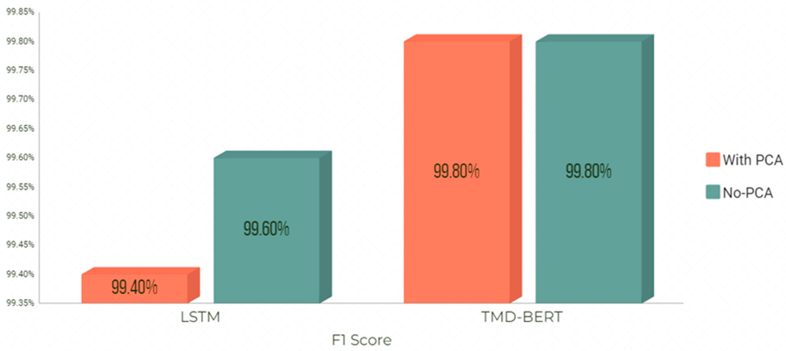
The experimental results indicated that TMD-BERT outperformed LSTM implementation. Figure 8 shows F1 Score for TMD-BERT compared with LSTM before and after dimensionality reduction with PCA, for both techniques.
PCA has not affected the TMD-BERT performance concerning F1 Score. Precision and Recall values remain unchanged, too, as depicted in Figure 9.
Figure 10 shows the average values of the actual transport media used, indicated by the blue line, and the predicted values indicated by the orange line. It is clear that the TMD-BERT model was able to capture the overall trend as the orange and blue lines coincide for the most part.
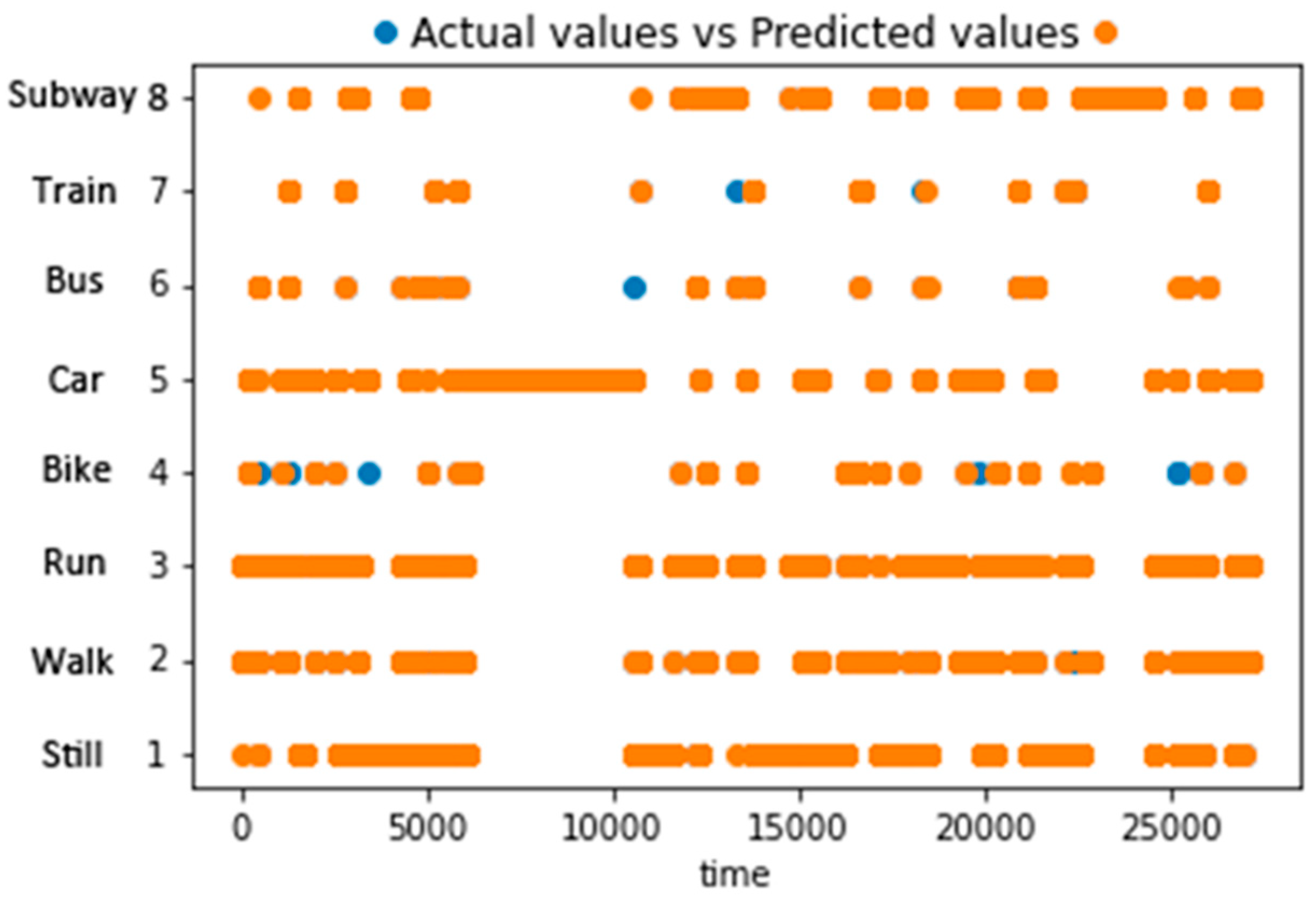
Similarly, the actual and predicted values per class are shown in Figure 11. The model does seem to provide an adequate fit in all classes.
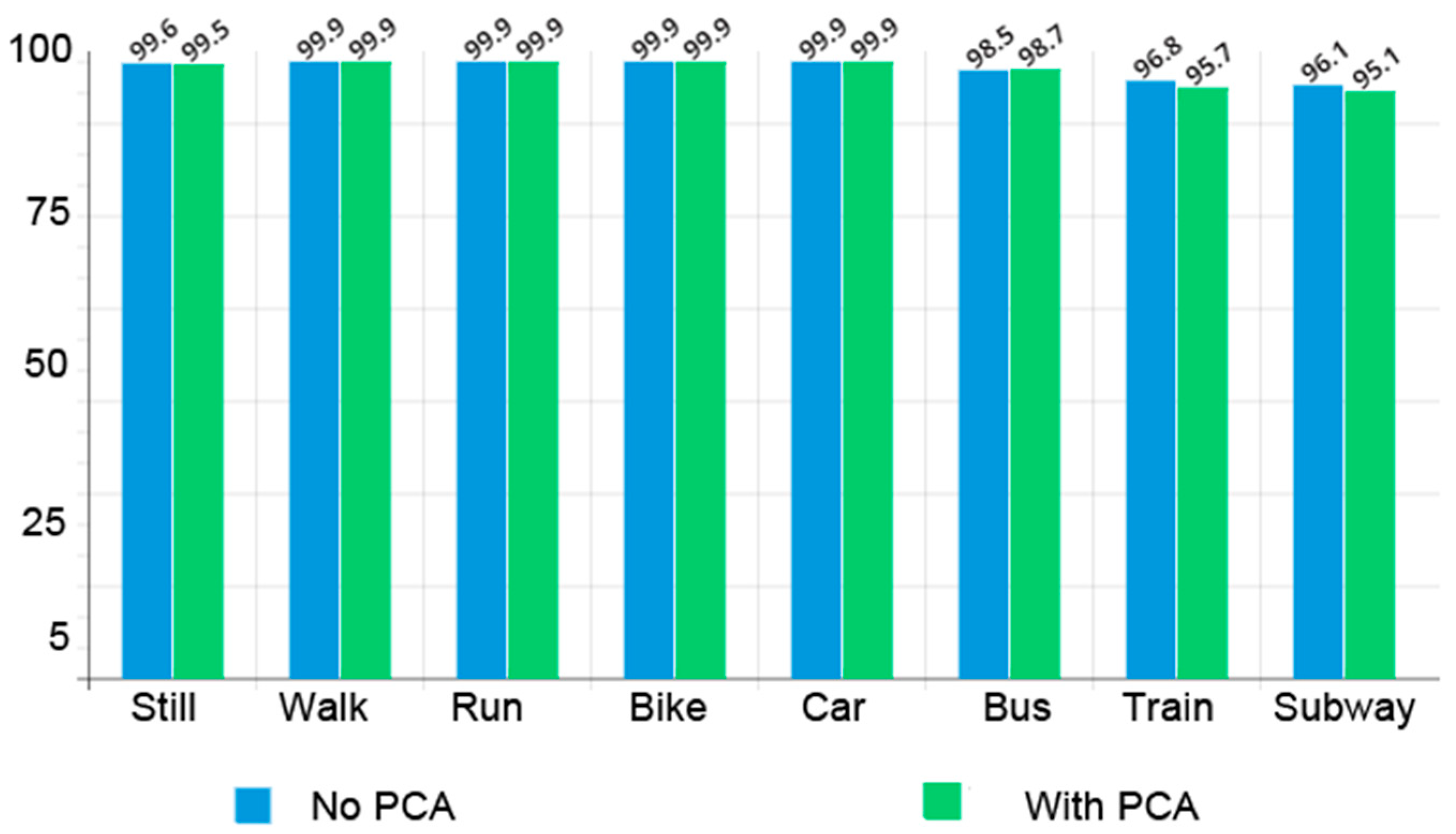
Figure 12 presents the accuracy per class before and after applying the PCA algorithm to our model. The classes Still, Train and Subway were predicted more accurately without dimensionality reduction and only Bus achieved an increase in accuracy after applying PCA. The prediction for the other classes (Walk, Run, Bike, Car) was almost perfect in both cases.
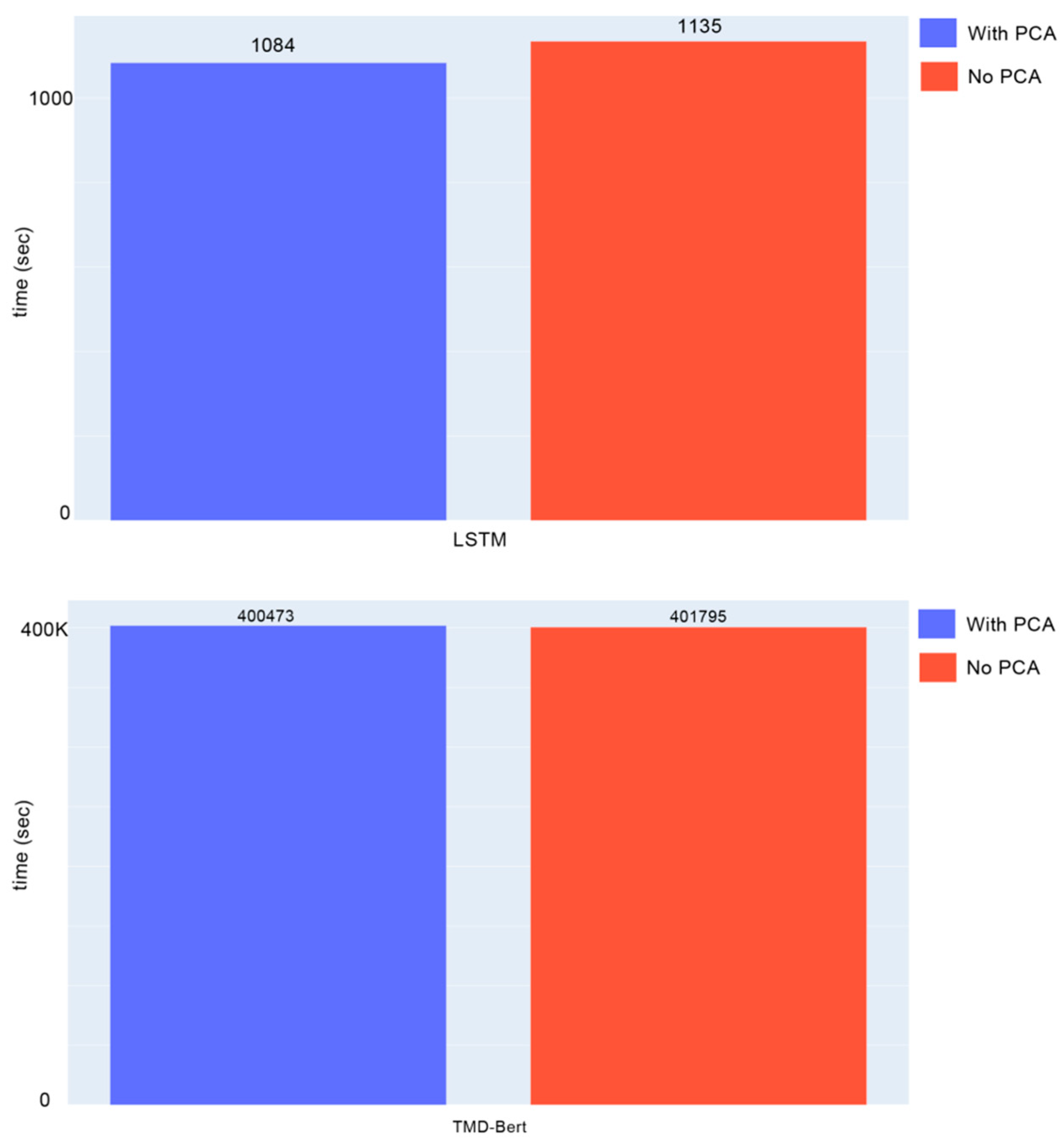
In terms of time, as depicted in Figure 13, TMD-BERT compared to LSTM had a longer training and prediction time, as the model ran on a CPU system. Here it should be noted that TMD-BERT can allow for massive parallelization of time series calculations and is thus far better able to take advantage of parallelism provided by modern GPU acceleration, thus significantly decreasing training time.
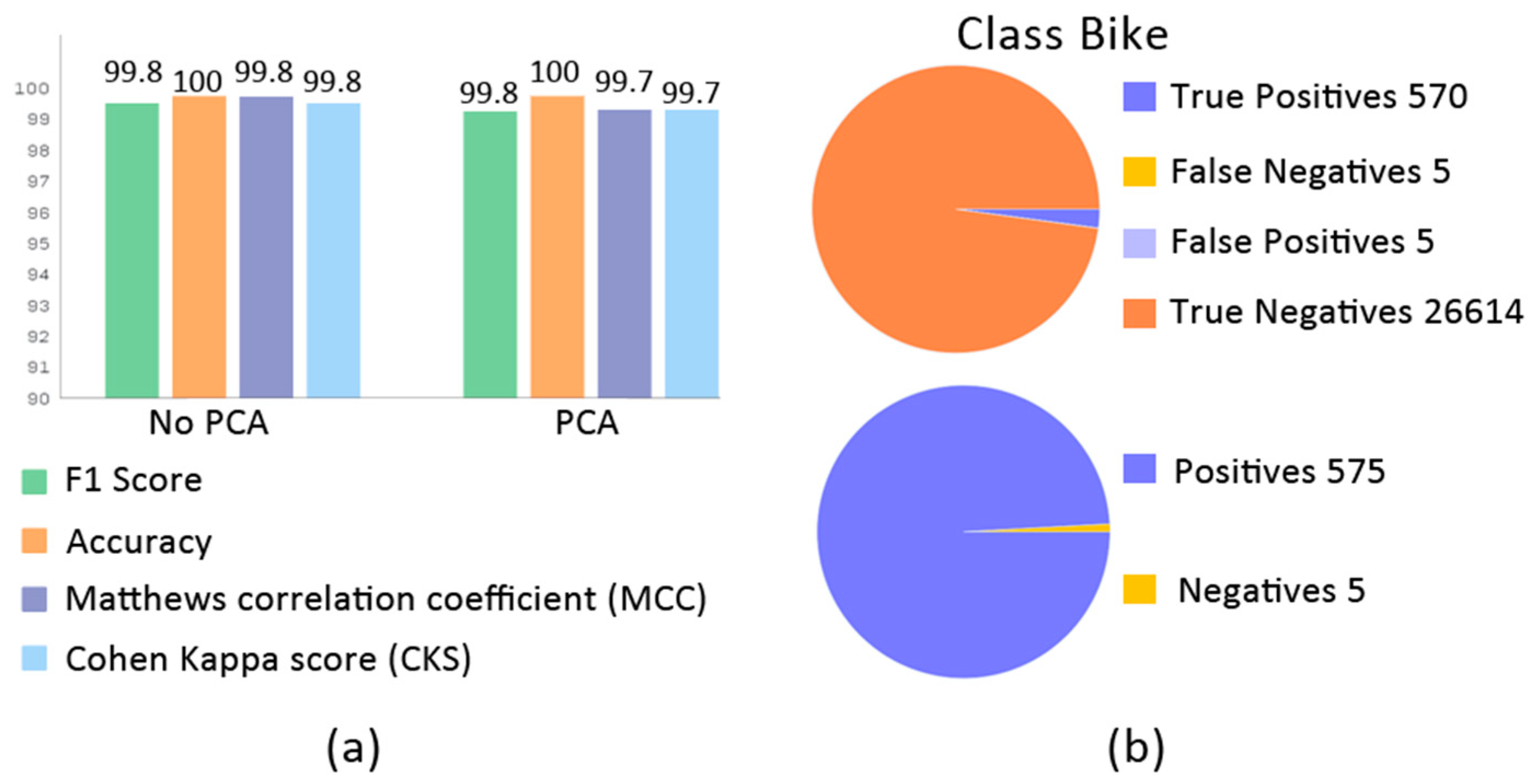
The Matthews correlation coefficient (MCC) [35] is a metric used widely in the NLP field to evaluate performance, especially for imbalanced classes. With +1 being the best score, and −1 the worst score, 0.997–0.998 value indicates a high performance of the model. Cohen Kappa Score (CKS) [36], a measure that can handle efficiently both multi-class and imbalanced class issues, can be defined as a metric used to compare the predicted labels deriving from a model with the actual data labels. The value ranges from -1 (indicating worst performance) to 1 (indicating best performance). A Cohen Kappa value of 0 means that the model is close to random guessing whereas a value of 1 means that the model is perfect [37]. A value of 0.997–0.998 indicates a high performance of the model. In Figure 14a, F1 Score, Accuracy, Matthews Correlation Coefficient (MCC), and Cohen Kappa Score (CKS) values before and after applying PCA, are depicted. True positives, False negatives, False positives, and True negatives values involved in the calculation of the above metrics, are shown in Figure 14b, being indicative of Bike class.

5. Conclusions

The automatic detection of transportation modes using mobile sensor data is a popular research problem whose outcome can be used further for support in several Intelligent Transportation System applications, but also for personalization and enhanced experience offered in mobile applications and service provision. Our proposed TMD-BERT model introduces the strengths of the bidirectional encoder representations from the transformers approach in the TMD problem, handling the entire sensor data sequence as a whole and thus allowing for better long-range dependency modeling. An extensive experimental evaluation shows the high performance of the model in comparison to the state of the art. Future directions of our work include the investigation of methods for increased interpretability of the provided framework, which at the same time retains an augmented degree of prediction accuracy regarding the estimated result.

Author Contributions

Conceptualization, I.D. and A.V.; methodology, A.V., P.M.; software, I.D.; validation, I.D. and A.V.; formal analysis, I.D., A.V. and D.G..; investigation, I.D. and A.V..; resources, G.M. and D.G.; data curation, I.D. and A.V.; writing—original draft preparation, I.D. and A.V.; writing—review and editing, I.D. and A.V.; visualization, I.D.; supervision, A.V., G.M. and D.G.; project administration, A.V. and G.M.,; funding acquisition, P.M. and G.M. All authors have read and agreed to the published version of the manuscript.

Funding

This research received no external funding.

Conflicts of Interest

The authors declare no conflict of interest.

References

  1. Drosouli, I.; Voulodimos, A.; Miaoulis, G. Transportation mode detection using machine learning techniques on mobile phone sensor data. In Proceedings of the 13th ACM International Conference on PErvasive Technologies Related to Assistive Environments (PETRA ’20), Corfu, Greece, 30 June–3 July 2020; Volume 65, pp. 1–8. [Google Scholar]
  2. Voulodimos, A.; Kosmopoulos, D.; Veres, G.; Grabner, H.; Van Gool, L.; Varvarigou, T. Online classification of visual tasks for industrial workflow monitoring. Neural Netw. 2011, 24, 852–860. [Google Scholar] [CrossRef] [PubMed]
  3. De Marsico, M.; Nappi, M. Face Recognition in Adverse Conditions: A Look at Achieved Advancements. In Computer Vision: Concepts, Methodologies, Tools, and Applications; IGI Global: Hershey, PA, USA, 2018. [Google Scholar] [CrossRef]
  4. Katsamenis, I.; Protopapadakis, E.; Voulodimos, A.; Doulamis, A.; Doulamis, N. Transfer Learning for COVID-19 Pneumonia Detection and Classification in Chest X-ray Images. In 24th Pan-Hellenic Conference on Informatics (PCI 2020); Association for Computing Machinery: New York, NY, USA, 2021; pp. 170–174. [Google Scholar] [CrossRef]
  5. Parasuraman, S.; Sam, A.T.; Yee, S.W.K.; Chuon, B.L.C.; Ren, L.Y. Smartphone usage and increased risk of mobile phone addiction: A concurrent study. Int. J. Pharm. Investig. 2017, 7, 125–131. [Google Scholar] [CrossRef] [PubMed]
  6. Mutchler, L.A.; Shim, J.P.; Ormond, D. Exploratory Study on Users’ Behavior: Smartphone Usage. In Proceedings of the 17th Americas Conference on Information Systems 2011, AMCIS 2011, Detroit, MI, USA, 4–8 August 2011. [Google Scholar]
  7. Servizi, V.; Pereira, F.C.; Anderson, M.K.; Nielsen, O.A. Transport behavior-mining from smartphones: A review. Eur. Transp. Res. Rev. 2021, 13, 57. [Google Scholar] [CrossRef]
  8. Drosouli, I.; Voulodimos, A.; Miaoulis, G.; Mastorocostas, P.; Ghazanfarpour, D. Transportation Mode Detection Using an Optimized Long Short-Term Memory Model on Multimodal Sensor Data. Entropy 2021, 23, 1457. [Google Scholar] [CrossRef] [PubMed]
  9. Vaswani, A.; Shazeer, N.; Parmar, N.; Uszkoreit, J.; Jones, L.; Gomez, A.N.; Kaiser, Ł.; Polosukhin, I. Attention Is All You Need. arXiv 2017, arXiv:1706.03762. [Google Scholar]
  10. Carpineti, C.; Lomonaco, V.; Bedogni, L.; Di Felice, M.; Bononi, L. Custom Dual Transportation Mode Detection by Smartphone Devices Exploiting Sensor Diversity. In Proceedings of the 2018 IEEE International Conference on Pervasive Computing and Communications Workshops (PerCom Workshops), Athens, Greece, 19–23 March 2018. [Google Scholar]
  11. Delli Priscoli, F.; Giuseppi, A.; Lisi, F. Automatic Transportation Mode Recognition on Smartphone Data Based on Deep Neural Networks. Sensors 2020, 20, 7228. [Google Scholar] [CrossRef]
  12. Liang, X.; Zhang, Y.; Wang, G.; Xu, S. A Deep Learning Model for Transportation Mode Detection Based on Smartphone Sensing Data. IEEE Trans. Intell. Transp. Syst. 2020, 21, 5223–5235. [Google Scholar] [CrossRef]
  13. Asci, G.; Guvensan, M.A. A Novel Input Set for LSTM-Based Transport Mode Detection. In Proceedings of the 2019 IEEE International Conference on Pervasive Computing and Communications Workshops (PerCom Workshops), Kyoto, Japan, 11–15 March 2019; pp. 107–112. [Google Scholar]
  14. Feng, Z.; Guo, D.; Tang, D.; Duan, N.; Feng, X.; Gong, M.; Shou, L.; Qin, B.; Liu, T.; Jiang, D.; et al. CodeBERT: A Pre-Trained Model for Programming and Natural Languages. arXiv 2020, arXiv:2002.08155. [Google Scholar]
  15. Lin, S.-Y.; Kung, Y.-C.; Leu, F.-Y. Predictive intelligence in harmful news identification by BERT-based ensemble learning model with text sentiment analysis. Inf. Process. Manag. 2022, 59, 102872. [Google Scholar] [CrossRef]
  16. Annamoradnejad, I.; Zoghi, G. ColBERT: Using BERT Sentence Embedding for Humor Detection. arXiv 2020, arXiv:2004.12765. [Google Scholar]
  17. Tarwani, K.M.; Edem, S. Survey on recurrent neural network in natural language processing. Int. J. Eng. Trends Technol. 2017, 48, 301–304. [Google Scholar] [CrossRef]
  18. Sherstinsky, A. Fundamentals of Recurrent Neural Network (RNN) and Long Short-Term Memory (LSTM) Network. Phys. D Nonlinear Phenom. 2020, 404, 132306. [Google Scholar] [CrossRef] [Green Version]
  19. Saxe, J.; Berlin, K. eXpose: A character-level convolutional neural network with embeddings for detecting malicious URLs, file paths, and registry keys. arXiv 2017, arXiv:1702.08568. [Google Scholar]
  20. Rumelhart, D.E.; Hinton, G.E.; Williams, R.J. Learning representations by back-propagating errors. Nature 1986, 323, 533–536. [Google Scholar] [CrossRef]
  21. Le, X.H.; Ho, H.V.; Lee, G.; Jung, S. Application of Long Short-Term Memory (LSTM) Neural Network for Flood Forecasting. Water 2019, 11, 1387. [Google Scholar] [CrossRef] [Green Version]
  22. Xiao, X.; Zhang, D.; Hu, G.; Jiang, Y.; Xia, S. CNN-MHSA: A convolutional neural network and multi-head self-attention combined approach for detecting phishing websites. Neural Netw. 2020, 125, 303–312. [Google Scholar] [CrossRef] [PubMed]
  23. Devlin, J.; Chang, M.; Lee, K.; Toutanova, K. BERT: Pretraining of deep bidirectional transformers for language understanding. In Proceedings of the NAACL HLT 2019—2019 Conference of the North American Chapter of the Association for Computational Linguistics: Human Language Technologies, Minneapolis, MN, USA, 2–7 June 2019; ISBN 9781950737130. Association for Computational Linguistics, Minneapolis, Minnesota. [Google Scholar]
  24. Chen, M.; Radford, A.; Wu, J.; Jun, H.; Dhariwal, P.; Luan, D.; Sutskever, I. Generative Pretraining From Pixels. In Proceedings of the 37th International Conference on Machine Learning 2020, Virtual, 13–18 July 2020. [Google Scholar]
  25. Chen, H.; Wang, Y.; Guo, T.; Xu, C.; Deng, Y.; Liu, Z.; Ma, S.; Xu, C.; Xu, C.; Gao, W. Pre-Trained Image Processing Transformer. In Proceedings of the 2021 IEEE/CVF Conference on Computer Vision and Pattern Recognition (CVPR), Nashville, TN, USA, 19–25 June 2021; pp. 12294–12305. [Google Scholar] [CrossRef]
  26. Carion, N.; Massa, F.; Synnaeve, G.; Usunier, N.; Kirillov, A.; Zagoruyko, S. End-to-End Object Detection with Transformers. In Proceedings of the European Conference on Computer Vision, Glasgow, UK, 23–28 August 2020. [Google Scholar]
  27. Jumper, J.; Evans, R.; Pritzel, A.; Green, T.; Figurnov, M.; Ronneberger, O.; Tunyasuvunakool, K.; Bates, R.; Žídek, A.; Potapenko, A.; et al. Highly accurate protein structure prediction with AlphaFold. Nature 2021, 596, 583–589. [Google Scholar] [CrossRef]
  28. Fuchs, F.B.; Worrall, D.E.; Fischer, V.; Welling, M. SE(3)-Transformers: 3D Roto-Translation Equivariant Attention Networks. arXiv 2020, arXiv:2006.10503. [Google Scholar]
  29. Xu, M.; Dai, W.; Liu, C.; Gao, X.; Lin, W.; Qi, G.; Xiong, H. Spatial-Temporal Transformer Networks for Traffic Flow Forecasting. arXiv 2020, arXiv:2001.02908. [Google Scholar]
  30. Jin, K.; Wi, J.; Lee, E.; Kang, S.; Kim, S.; Kim, Y. TrafficBERT: Pre-trained model with large-scale data for long-range traffic flow forecasting. Expert Syst. Appl. 2021, 186, 115738. [Google Scholar] [CrossRef]
  31. Kingma, D.P.; Ba, J. Adam: A Method for Stochastic Optimization. International Conference on Learning Representations. arXiv 2014, arXiv:1412.6980. [Google Scholar]
  32. Vig, J. A Multiscale Visualization of Attention in the Transformer Model. arXiv 2019, arXiv:1906.05714. [Google Scholar]
  33. Madabushi, H.T.; Kochkina, E.; Castelle, M. Cost-Sensitive BERT for Generalisable Sentence Classification on Imbalanced Data. arXiv 2019, arXiv:2003.11563. [Google Scholar]
  34. Edwards, A.L. The Correlation Coefficient. In An Introduction to Linear Regression and Correlation; W. H. Freeman: San Francisco, CA, USA, 1976; pp. 33–46. [Google Scholar]
  35. Chicco, D.; Jurman, G. The advantages of the Matthews correlation coefficient (MCC) over F1 score and accuracy in binary classification evaluation. BMC Genom. 2020, 21, 6. [Google Scholar] [CrossRef] [Green Version]
  36. Cohen, J. A coefficient of agreement for nominal scales. Educ. Psychol. Meas. 1960, 20, 37–46. [Google Scholar] [CrossRef]
  37. Landis, J.R.; Koch, G.G. The measurement of observer agreement for categorical data. Biometrics 1977, 33, 159–174. [Google Scholar] [CrossRef] [PubMed]
Figure 1. The model structure.
Electronics 12 00581 g001
Figure 2. The fine-tuning procedure for sequence classification tasks.
Electronics 12 00581 g002
Figure 3. (a) Attention for the input text “−0.38 0.19 −0.22 0.36 0.38 0.55 0.54” with attention head 11 (orange) and layer 3 selected; (b) Attention for the input text “0.03 0.37 −0.34 −0.55 0.04 0.58 0.23” with attention head 5 (brown) and layer 3 selected; (c) Attention for the input text “−0.38 0.19 −0.22 0.36 0.38 0.55 0.54” and “0.03 0.37 −0.34 −0.55 0.04 0.58 0.23” with attention head 0 (blue), layer 9 and Sentence A → Sentence B selected.
Electronics 12 00581 g003
Figure 4. The attention in all the heads for the input text “−0.38 0.19 −0.22 0.36 0.38 0.55 0.54” and “0.03 0.37 −0.34 −0.55 0.04 0.58 0.23”.
Electronics 12 00581 g004
Figure 5. The distribution of sensor measurements.
Electronics 12 00581 g005
Figure 6. A correlation analysis using Pearson’s Correlation Coefficient (PCC).
Electronics 12 00581 g006
Figure 7. The number of principal components for PCA algorithm.
Electronics 12 00581 g007
Figure 8. F1 Score for TMD-BERT compared with LSTM, before and after dimensionality reduction with PCA.
Electronics 12 00581 g008
Figure 9. Precision and Recall for TMD-BERT before and after dimensionality reduction with PCA.
Electronics 12 00581 g009
Figure 10. This is a figure. Schemes follow the same formatting.
Electronics 12 00581 g010
Figure 11. The actual and predicted values per class without dimensionality reduction.
Electronics 12 00581 g011
Figure 12. The accuracy per class before and after applying PCA.
Electronics 12 00581 g012
Figure 13. Training time for LSTM and TMD-BERT with and without PCA.
Electronics 12 00581 g013
Figure 14. (a) F1 Score, Accuracy, Matthews correlation coefficient (MCC) and Cohen Kappa Score (CKS) values before and after applying PCA (b) True positives, False negatives, False positives, True negatives for Bike class.
Electronics 12 00581 g014
Table 1. The parameters of the TMD-BERT model.
TMD-BERT Model
DataLoaderRandomSampler (for train data)
SequentialSampler (for test data)
Batch size1
epochs1
OptimizerAdam
Learning rate 0.00001
epsilon0.00000001
Schedulerget_linear_scheduler_with_warmup
Table 2. Samples per class.
ClassSamples
Still19,085
Walk46,987
Run39,814
Bike43,988
Car26,268
Bus3,861
Train623
Subway693
Table 3. The parameters of LSTM.
LSTM hyperparametersValues
Num of neurons in the first layer64
Output values8
OptimizerAdam
Dropout0.2
Learning rate0.001
Error calculationCategorical cross-entropy
Dense Layer1
Activation functionSoftmax
Disclaimer/Publisher’s Note: The statements, opinions and data contained in all publications are solely those of the individual author(s) and contributor(s) and not of MDPI and/or the editor(s). MDPI and/or the editor(s) disclaim responsibility for any injury to people or property resulting from any ideas, methods, instructions or products referred to in the content.