Abstract
Ethylene-Vinyl Acetate (EVA) copolymer was synthesized from ethylene and vinyl acetate at high temperatures and ultra-high pressures. In this condition, any reactor disturbances, such as process or mechanical faults, may trigger the run-away decomposition reaction. This paper proposes a procedure for constructing a conditional health status prediction structure that uses a virtual health index (HI) to monitor the reactor bearing’s remaining useful life (RUL). The piecewise linear remaining useful life (PL-RUL) model was constructed by machine learning regression methods trained on the vibration and distributed control system (DCS) datasets. This process consists of using Welch’s power spectrum density transformation and machine learning regression methods to fit the PL-RUL model, following a health status construction process. In this research, we search for and determine the optimum value for the remaining useful life period (TRUL), a key parameter for the PL-RUL model for the system, as 70 days. This paper uses four-fold cross-validation to evaluate seven different regression algorithms and concludes that the Extremely randomized trees (ERTs) is the best machine learning model for predicting PL-RUL, with an average relative absolute error (RAE) of 0.307 and a Linearity of 15.064. The Gini importance of the ensemble trees is used to identify the critical frequency bands and prepare them for additional dimensionality reduction. Compared to two frequency band selection techniques, the RAE and Linearity prediction results can be further improved to 0.22 and 8.38.
1. Introduction
Ethylene-Vinyl Acetate (EVA) is a thermoplastic polymer formed by the copolymerization of ethylene and vinyl acetate (VA). The product specifications can be adjusted by molecular weight and vinyl acetate content. EVA is a popular material for solar encapsulation films and is widely used in foam materials [1]. EVA resin can be manufactured using either the autoclave or tubular methods. Compared with the tubular form, the autoclave method can produce a high degree of long chain branch (LCB) and broad molecular weight distribution (MWD) and can offer VA concentrations beyond 30%. The autoclave method operates around 1800 to 2000 atm (atmospheres), with the reaction temperature ranging between 160 and 200 °C. The run-away decomposition conditions depend on reactor pressure [2], temperature, mechanism of ignition, and vinyl acetate ratio [3]. Decomposition may occur when mechanical faults in the reactor, such as bearing failures or other sources of mechanical friction, produce a hot spot [4]. Once decomposition occurs, the reactor will quickly produce a large amount of methane and hydrogen, increasing the reactor pressure. When the reactor reaches the warning pressure of the safety rupture disc, it will purge and rapidly discharge reactants into the environment, causing a series of pollution and even severe industrial safety hazards.
The decomposition reaction would damage equipment, cause production losses, and entail fines from the government, and is hazardous for the operators. However, current autoclave reactor modeling only focuses on predicting MWD [5] and melting index (MI) [6]. Therefore, prediction maintenance of the bearing for the ultra-high pressure autoclave reactor remains an important issue.
Machine learning is the study of utilizing algorithms and statistical models to make predictions based on past data, and has been used in a variety of domains. Recent machine learning research includes optimizing syngas engine operating parameters [7], developing predictive maintenance support systems [8], predicting drug-drug interaction [9], protein identification [10] and remaining useful life of lithium-ion batteries [11]. Bearing health status classification and remaining useful life (RUL) prediction is a popular research field and there is a comprehensive review [12]. Acceleration time series, transformed frequency domain, and time-frequency analysis are commonly used to predict bearing health. The power spectral density (PSD) is shown to outperform the discrete Fourier transform (DFT) in providing better features in the frequency domain [13], and the Welch method based on time averaging over short periodograms to calculate the Welch PSD has been provided in [14]. The Welch PSD can then be used to generate valuable features for health status classification using multiple machine learning methods such as bagging support vector machine (SVM) [15] and radial basis function (RBF) neural network [16]. Standard deviation, kurtosis, variance, peak-to-peak, and other statistical features are common for further predictions and are calculated from time-series and frequency domain data [17]. The Weibull distribution is often used to smooth oscillating statistical features over time [18]. Some also use large machine learning models such as deep convolution neural networks (CNN) to extract features from wavelet transforms [19]. At the same time, traditional machine learning models such as SVM are still popular methods for predicting RUL or detecting failure [20]. More complicated prediction methods, such as recurrent neural networks (RNN) [21], deep CNN [22], auto-encoder [23], and long short-term memory (LSTM) [24], have been used to predict RUL. Ensemble techniques can further boost the performance for bearing health problems [25]. Ensemble decision trees methods such as eXtreme Gradient Boosting (XGboost), gradient boost, and adaptive boosting can classify bearing health status [26]. The Gini importance of the ensemble trees, such as random forest [27], and adaptive boosting [28], can be used to calculate the significance of selected features for later predictions. Some researchers have demonstrated that ensemble tree methods and SVM provide greater accuracy than some RNN designs [29].
A defect initiation stage with a small defect is found by modeling the bearing wear evolution [30]. This characteristic is also found using the geometry of a health indicator (HI) [31], and the piecewise linear RUL (PL-RUL) model proposed in [32] is often used as a predicting model to fit the phenomenon.
Even though many studies on bearing health status classification and RUL prediction are already available, this research is valuable due to the following reasons:
- ■
- This research focuses on a complex ultra-high pressure and special lubricating system with multiple product grade transitions. Moreover, inappropriate operation can lead to the run-away decomposition of the process, which may cause serious harm to people and the environment.
- ■
- Past supercritical ultra-high pressure autoclave reactor modeling only focuses on predicting MWD [5] and MI [6]. Therefore, prediction maintenance of the ultra-high pressure autoclave reactor bearing remains an important issue.
- ■
- Most studies focus on data from small-scale laboratory experiments or a few public databases [12], such as the NASA CMAPSS dataset [33] and the PHM 2012 prognostic challenge [34]. This study focuses on real-world data and increases the diversity of the dataset in this field.
- ■
- Most bearing life predictions are based solely on accelerometer data. The DCS data, such as motor current, provided in real-world processes, is rarely used. This study combines datasets from different domains to produce a more holistic as well as accurate prediction.
- ■
- While traditional dataset processing time series data employs dozens of statistical features to make predictions, these features are frequently challenging to interpret and lack physical intuition. A more intuitive approach is to find and monitor characteristic frequencies or frequency bands. For example, compare the time-frequency analysis with the calculated theoretical values [35], or look into the characteristic frequency band with high monotonicity over time [36]. In this paper, we utilize machine learning approaches to select characteristic frequency bands for predicting the remaining useful life of the bearing.
- ■
- Our dataset is sparse and limited (one day, one datum, 426 days, four life cycles). Complex approaches such as CNN and LSTM are not suitable for this small set of data. In this study, we emphasize simple methods and the addition of process data (motor three-phase current).
- ■
- This is the first time this dataset has been used in a predictive maintenance analysis in terms of machine learning and AI. As a result, there is no published work on the same or similar problem or data to compare. Therefore, to build a solid foundation for future studies, we reviewed several commonly used regression methods rather than focusing on ensemble architectures, which might generate better results.
- ■
- This study also aids the industry in the implementation of a predictive maintenance plan, which increases production efficiency while preventing hazardous pollution. This is very much in line with Sustainable Development Goal (SDG) Target 8.8, which promotes a safe working environment for those in precarious employment, and SDG Target 9.4, which encourages industry to upgrade for sustainability.
This study is an industry-sponsored project that makes use of data from an operating supercritical ultra-high pressure reactor that was provided by an anonymous company. Because the training dataset is a private asset of the company, disclosing the data is not possible.
On the other hand, rather than focusing on the systems presented in the paper, we believe that the value of this study is in developing a general procedure that can be used to build predictive maintenance models for similar systems. Different systems also have their own limitations and challenges, which may lead to selection of different models and parameters. Therefore, we have clearly explained the model-building process step by step in the Methods section, and we hope the readers can follow the procedure to build their own models based on their own custom dataset.
2. Process Description and Methods
2.1. Process Description
The autoclave process flow and the reactor configuration diagram are given in Figure 1. A compressed ethylene monomer stream uses two large reciprocating compressors connected in series to reach the high reaction pressure. The primary compressor can increase the ethylene feed pressure from 40 atm to approximately 200 atm. The secondary compressor can raise the pressure of the mixture of ethylene, vinyl acetate, and chain modifier to around 1800 to 2000 atm. The high-pressure mixed stream enters the reactor with an initiator and modifiers and undergoes free-radical bulk copolymerization with a reaction temperature between 160 and 200 °C. A separator vessel will separate the molten EVA polymer from the unreacted mixture. Depending on the pressure level, it will recycle to the first or second compressor after removal. The molten EVA polymer will be removed from an extruder and then pelleted and bagged.
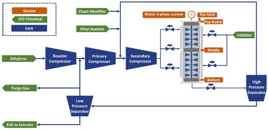
Figure 1.
Process schematic of the EVA plant and the reactor configuration diagram.
The reactor includes four vibration sensors, and the motor current is recorded in the DCS historian, shown in Figure 1. The top axial and radial accelerometers are used to monitor the motor bearing, and the other two radial accelerometers are used to monitor the middle and bottom bearings. The height of the reactor is around 7 m. The reactor bearing is encased in the reactor, and the polymer within the reactor serves as a lubricant. Due to the high pressure, the thickness of the reactor exceeds 10 cm. The thick wall prevents accelerometers from being mounted closest to bearings and may absorb or reflect the vibration sensor’s characteristic frequency, making it challenging to analyze the early signals for any bearing anomaly.
2.2. Method
The process flow of the Condition-Based Maintenance structure of the EVA reactor is shown in Figure 2. There are four stages in the process flow: (1) data acquisition (highlighted in blue), (2) health index (HI) construction (highlighted in yellow), (3) health status (HS) division (highlighted in green), and (4) bearing reliability prediction (highlighted in gray).
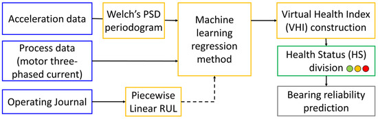
Figure 2.
Process flow of the Condition-Based Maintenance of the EVA reactor.
2.3. Data Acquisition
At this stage, four accelerometers are installed on four different parts of the stirred tank reactor, including the top axial, top side, middle side, and bottom side. These sensors detect vibration motion and record acceleration time series data for subsequent analysis. The collected time-series data is sampled every day and lasts 3.2 s at a sampling rate of 2560 Hz. In this study, we performed cross-validation across four events totaling 426 days. Each sensor’s time-series data size is 8192 sample points per day, for a total of 3490k. These four sensors have a total data size of 13,959 k. The motor current is obtained using DCS historian. In this research, two types of dataset are used, the acceleration (A) dataset and acceleration plus the motor current (A/C) dataset.
2.4. HI Construction
The Health Index (HI) construction approach combines four acceleration time-series data with physical meanings into a virtual health index using frequency analysis and various machine learning regression methods. The HI construction stage is subdivided into three phases. First, we use Welch’s method to convert each sensor’s time series data into a power spectral density (PSD) periodogram. Second, we use the PL-RUL model to create a bearing life training dataset. Finally, we test various regressors on the training dataset and choose the best-fit regressor setup.
2.4.1. Welch’s Method
As shown in Figure 3, the time-domain data of the top axial sensor on day 0 was collected within 3.2 s with a sampling frequency of 2560 Hz, and 8192 acceleration values were collected with the unit of g (9.80665 m/s2). This illustrative time-domain data is highly oscillating; it may thus be challenging to find useful characteristic features for this system. On the other hand, the PSD periodograms show the power amplitude of a given frequency band in a range of given frequencies, which aids in constructing characteristic frequency patterns. The PSD is calculated using Welch’s method [14], as illustrated in Figure 4, which shows the PSD periodogram computed using the traditional method and Welch’s method with a window size of 512 per segment, smooth, and containing the trend of the original method.
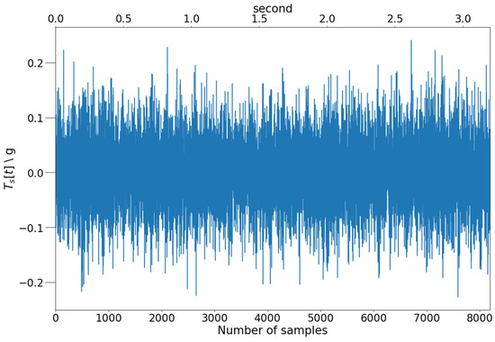
Figure 3.
Time series data from a top axial sensor () on a certain day.
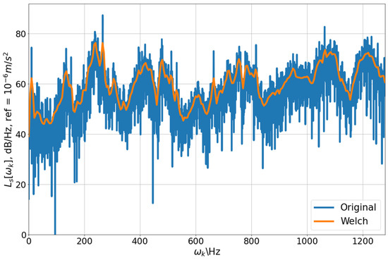
Figure 4.
Power spectral density periodogram level from reactor top axial sensor () on a certain day. Reference at .
Calculating PSD periodograms using Welch’s method is a standard procedure for converting time-domain data to frequency-domain data. This method calculates the power average PSD of the signal and has three advantages over the discrete Fourier transform. First, PSD normalizes the results for the different durations and sampling rates, making the results comparable across time-series data with different sampling rates and durations. As a result, Welch’s method can accept source data with varying sampling frequency and duration while producing results with the same dimension, which is impossible with traditional PSD calculation procedures. This feature makes our procedure more adaptable in practice. For example, we can change sensors with different sampling frequencies or adjust sampling duration without reconstructing our conditional-based structure. Second, by smoothing the highly oscillating frequency domain data while retaining the original method’s trend, this method balances the fluctuation and resolution of the periodogram, as shown in Figure 4. Finally, the output dimension is reduced, and the reduced ratio can be tuned. Most of the results reduced the size by 16-fold if not otherwise specified. The following describes the calculation for the power spectral density periodogram using Welch’s method.
Suppose is a discrete sequence of the acceleration time-domain data with a length collected by the sensor , where . The time series data is a function of time that conveys information on the vibration acceleration with unit equals (i.e., ) and a sampling frequency . Define zero-padded time series referenced at as stated in the Equation (1). Zero-padding is to generalize from range to all integer numbers, and aref referenced at is commonly used for acceleration data.
After defining , we split it into overlapping segments. We detrend the data to remove extremely low-frequency components in each segment, and a window function is applied to prevent leakage. Following, we define segmented, constant detrended, windowed, and zero-padded time series as , shown by the Equation (2):
where is the index in each segment, and ; is the segment index, and ; is the size of each segment, and is the number of segments. This process extracts unwanted noise from the signal [37]. Furthermore, is the Hanning window function of length , shown in the Equation (3):
Further, is the inter-segment overlapping ratio and equals 0.5 and 1 for Welch’s and Bartlett’s methods, respectively.
Suppose is the periodogram of the block shown in Equation (4) or Equation (5), which is the absolute square of the Fast Fourier Transform (FFT) results corrected by the window energy correction factor , and a one-sided factor of 2 is applied to Equation (5). If the window function is box-window, , which equals the Parseval’s Theorem correction factor. k is the frequency index, which are the integers from to .
If the value of M is odd for , , or the value of M is even for , where m = 0, 1, …, M − 1, then:
For other values of , where m = 0, 1, …, M − 1, then:
The below-stated Equation (6) can convert the frequency index to the actual frequency .
Welch’s power spectral density periodogram is expressed by , the average of the M power spectral density periodograms. This is stated in Equation (7) below for k = 0, 1, …, [N/2].
The vibration acceleration level with k = 0, 1, … , [N/2], and for the sensor is stated in Equation (8).
The Welch method significantly reduced the PSD periodogram’s size from 4096 to 257 (N/2 + 1, where N is set as 512), and the periodogram is less oscillatory while maintaining its trend.
2.4.2. Piecewise Linear Remaining Useful Life (PL-RUL)
The remaining useful life (RUL) is the useful life left of the bearing at a particular operation period. It is represented in a linear line with a slope equal to −1. In this study, the remaining useful life () is defined as the time from the current time () until the end of use of the bearing (). This approach assumes the bearing’s health status on the last day is the same, which is slightly off the mark but a reasonable assumption. Another challenge is predicting the RUL at an early stage. In the early stage, the RUL in different events gives varying results due to different operation periods, but the bearings are new and not yet seriously degraded. This makes the prediction of the RUL difficult. Therefore, we adopt the modified form of the RUL model known as the piecewise linear RUL model () [32], whose life diagram is shown in Figure 5. This model comprises two straight lines: a horizontal line with a height equals before the first predicting time () and a linear RUL line with a slope of −1 between and . The following Equation (9) describes the PL-RUL model:
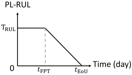
Figure 5.
Piecewise linear remaining useful life diagram, where is the tuning parameter called the remaining useful life period, is the first predicting time when the first RUL predicting occurs and is the end of use time for bearing.
The horizontal line indicates that we have given up predicting the precise lifespan in the early stage but have identified the status as “healthy.” We resume prediction when the expected number of days is less than the remaining useful life period (), which is also the model tuning parameter and has a relationship of . This approach is reasonable because it is difficult to predict in the early stages when the degradation is negligible.
2.4.3. Regression
In our case, each sensor has 257 frequency bands. Four sensors add up to 1028 nodes in the input. The selected regressor takes 1028 inputs, representing the PSD level determined by Welch’s method. It is trained on the bearing piecewise RUL of that specific day to minimize the mean square error.
This is the first time this dataset has been used in a predictive maintenance analysis in terms of machine learning and AI. Moreover, similar ultra-high pressure systems have not been investigated yet. Although all machine learning models can predict the remaining useful life of the bearing to a certain degree, their performance varies. As a result, we are motivated to seek out the most appropriate and effective methods and offer guidance to future researchers as well as practitioners.
Seven commonly used regressors were tested using Scikit-learn [38], including linear regression, support vector regression, extremely randomized trees regression [39], random forest regression [40], Adaboost regression [41], Gradient boost regression [42], and eXtreme Gradient Boosting (XGboosts) regression [43]. Extremely randomized trees (ERTs) has piecewise linear geometry [39] and is believed to perform better for piecewise linear functions. This method is similar to bagging trees; it uses extremely randomized trees instead of decision trees, randomly selecting a single attribute and cut-point at each node.
As mentioned above, our regression model takes in more than 1000 input variables, making it difficult to train and interpret. Therefore, selecting key variables and reducing the number of variables can help build smaller but more precise, stable, and interpretable models. One of the methods to select variables is to calculate the Gini importance of each feature in the ensemble trees. The method assists in determining which features (frequency bands) are potentially important in predicting the health index and provides knowledge or vision to on-site engineers. The Gini importance for specific features is calculated using Scikit-learn [38], and the process is as follows: First, compute the regression mean square errors (MSE) of each node, which is the node’s mean square error. Second, compute the decreased MSE for each node. This also means that the MSE of adding a node is reduced. Finally, the MSE of each node is normalized to a sum of 1, and the Gini importance for a specific feature is the sum of the nodes using the features to make decisions.
The predicted results of the regressor are the bearing’s PL-RUL. To ensure that each event has the same data size, we randomly oversample 350 data points in each of the 4 events.
2.4.4. Reliability Regression Results Evaluation
The prediction results must be evaluated to determine which set of hyper-parameters, regression algorithms, and target function selection is best. Mean squared error (MSE) is a popular measurement tool. However, MSE inherently magnifies the error for large values. As a result, we used relative absolute error (RAE) to solve the problem. The following Equation (10) describes how the RAE is defined:
where and represent the actual targets and their average, represents the predicted target.
Another evaluation parameter we use is Linearity, defined as the predicted linear RUL line’s mean squared error to its linear fit. The parameter evaluates the linear trend of the RUL line. A high degree of oscillation in the prediction may cause false alarms and confusion for the on-site engineers; therefore, we also value the consistency of the trend.
2.5. Health Status (HS) Division
The Health Status could be easily created by applying a suitable threshold to the regression results to predict the virtual health index (HI), which is further classified into different states. However, this approach is too sensitive to be used on-site. A time-relevant approach is added to improve system reliability, and the status of Normal, Warning, and Danger is described. The deterioration of the state happens only when the estimated reliability surpasses the threshold three times in a row. A monotonic decreasing function for the health status trend is also obtained by the design of this health status division method. It becomes an essential feature for predicting health status, which deteriorates over time.
2.6. Bearing Reliability Prediction
Bearing reliability prediction is similar to the HI construction and health status division processes. Welch’s approach is used to determine the PSD level using data collected by four sensors for 3.2 s at a sampling rate of 2560 Hz. The PSD level values and process data are fed into a trained machine learning regressor to predict a reliability value. Finally, the reliability and two previous values are compared to the threshold to determine if the bearing status is normal, warning, or dangerous.
2.7. Limitation
The prediction obtained from this study should be carefully reviewed, and we have listed the study’s limitations:
- ■
- This study’s sample size is small compared to other regularly used datasets. This study’s system is an ultra-high-pressure reactor containing polymers with a broad distribution of molecular weight. This characteristic shows that the bearing functions in a variety of conditions and the method of failure are likely to vary. The dataset may not account for all potential failure mechanisms. Consequently, if a new failure mode occurs, it may be necessary to retrain the machine learning model.
- ■
- The sampling interval for this study is once per day. Therefore, it is difficult for the model to respond to short-term events such as grade transitions. In addition, short-term events may contaminate the training dataset, causing the results to deviate from the correct long-term trend.
3. Results and Discussion
3.1. Training Using Acceleration and Motor Datasets
In this study, the cross-validation method for four events shown in Table 1 is used. In the ith cross-validation trial, we test the ith event and train using 350 oversampling on each of the other three events. For instance, in trial 1, we randomly choose 350 samples from each of events 2, 3, and 4 to train on before validating them in event 1.

Table 1.
Events for cross-validation.
The study uses two datasets: the acceleration (A) dataset and the acceleration plus motor current (A/C) dataset. Figure 6 and Figure 7 depict the prediction results using 4-fold cross-validation trained by ERTs based on two different datasets. The color of each prediction point represents the health status (green for normal, orange for warning, and red for danger). The warning and danger status threshold is manually given to be 40 and 20 days. The two models’ predictions have similar relative absolute loss values (A: 0.301, A/C: 0.307) and Linearity (A: 16.715, A/C: 15.064). It is challenging for the model to utilize the motor datasets, which are 340 times smaller than the acceleration datasets.
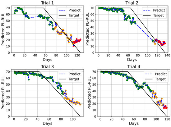
Figure 6.
4-Fold cross-validation results with days for trials 1 to 4 using A/C dataset, using Extremely randomized trees optimal Linearity setting (n_estimators = 100, max_depth = None, min_samples_leaf = 2, min_samples_split = 10).
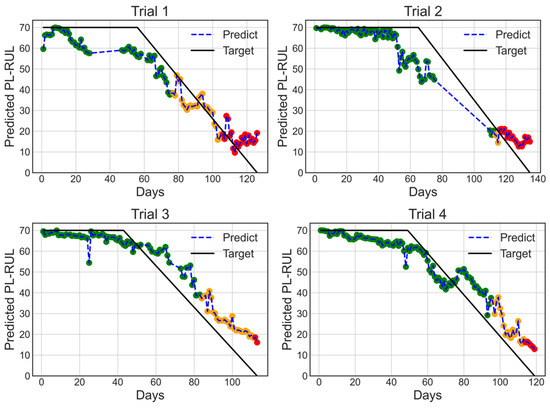
Figure 7.
4-Fold cross-validation results with days for trials 1 to 4 using A dataset, using Extremely randomized trees optimal Linearity setting (n_estimators = 100, max_dept h = None, min_samples_leaf = 2, min_samples_split = 10).
The results show that our prediction curve fits well. The predictions transition smoothly from normal to warning and warning to danger. However, we found that the stated curve can predict neither values larger than 70 days nor fewer than 10 days. The nature of the decision tree regression explains the upper bound of 70 days. The regression tree predicts based on average results. Because no training sample is larger than 70 days, no prediction result will be greater than 70 days. The lower bound of 10 days may imply that the breakdown behavior varies depending on the case. The predicted results remained at 10 days because no testing event’s breakdown behavior is highly correlated to other training events.
We have trained the models under the same parameters ten times to obtain the variance between models. The results of the RAE standard deviation of the above two ERTs models are both 0.006, and the Linearity standard deviations are 1.277 (A/C) and 0.967 (A). The values of the variance are low, indicating the model can be successfully trained recursively, and because of the random nature of the ERTs model, we believed there was little over-fitting concern.
3.2. Training Using Different Regression Methods
To fit the piecewise RUL function, seven regression methods were investigated, and the comparison and hyperparameter tuning are shown in Table 2. Four-fold cross-validation for each trial is performed on the AC dataset, as described in the Methods section, where RAE and Linearity were calculated for each test case and averaged for further evaluation. For each method, we performed the grid search on hyperparameters to get the best results in terms of lower RAE and Linearity. The results show that the XGBoost Regression method achieves the lowest average RAE, while the ERTs method has the lowest Linearity. Figure 8 shows the XGBoost prediction results with the A/C dataset using the XGBoost regressor. In this four-fold cross-validation, the color of each prediction point represents the health status (green for normal, orange for warning, and red for danger). The warning and danger status thresholds are manually given to be 40 and 20 days.
Table 2.
Comparison of seven regression methods using cross-validation with days trained on A/C dataset. The best averaged RAE and Linearity results and the parameters are obtained through grid search for each algorithm, and the grid search range is also specified in the table.
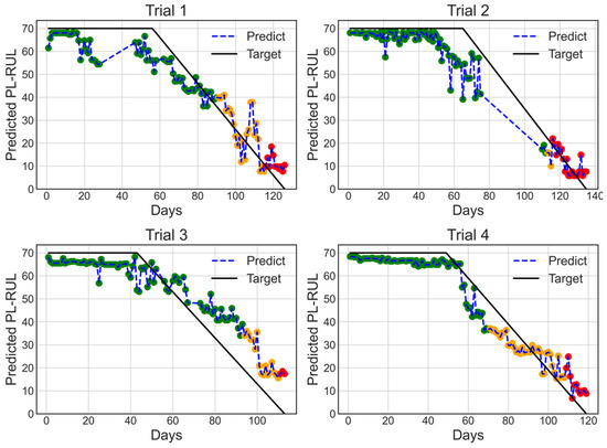
Figure 8.
4-fold cross-validation results with days for trials 1 to 4 using A/C dataset and XGBoosting regressor with optimal regressor settings (min_child_weight = 10, gamma = 1.5, n_estimators = 50, colsample_bytree = 0.6, max_depth = 4).
Although XGBoost seems more effective at minimizing RAE loss and has the lowest RAE value of 0.272, it has a significant drawback. The XGBoost prediction is staircase-like, and the piecewise RUL is either predicted to drop abruptly in a short period or to remain constant over an extended length of time. The XGBoost prediction is less linear at the linear RUL phase when compared to ERTs, which can be demonstrated by comparing the Linearity (mean squared error of the slope phase to its linear fit). The ERTs’ average Linearity is the lowest of all, which is 15.064, while XGboost is 24.381. In practice, a low Linearity index is critical for the predicted results. The on-site engineers may need clarification if the expected days show a significant fluctuation or sudden decrease. Other ensemble trees regression methods such as Gradient boost, Adaboost, and Random forest exhibit similar stair-case-like phenomena. Only the best Linearity ERTs can achieve both low RAE and Linearity.
3.3. Parameter Selection
Every system has its characteristic remaining useful life period (). An analysis was performed to search from small to large to determine the best-fit value in this study. The following procedures were applied to find the best value. Initially, choose a value of and construct the PL-RUL function. In the next step, the dataset is run through 4-fold cross-validation, and RAEs are recorded. Finally, another value is selected. We repeated these stepsto search the space for the smallest RAE fit. Figure 9 illustrates the outcome of the process.
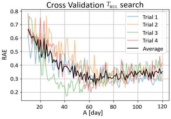
Figure 9.
Optimal search from 10 days to 120 days evaluated using RAE. Each data point represents the RAE of an ERTs with 10 estimators trained on A/C combined dataset.
All four trials have a local minimum, indicating that an optimum exists for the piecewise linear RUL function. In the 4 different trials, however, the optimum values of range from the 40s to the 80s, making it difficult to conclude the optimum value of from the best-fit viewpoint. Due to ERTs’ random construction, the result trends likewise varied significantly. In response to the abovementioned considerations, RAEs from the four trials are averaged, and the average curve trend reaches a minimum at about 70 days, which results in choosing 70 days as the value in this study.
3.4. Gini Importance
Model interpretation is an important part of today’s machine learning research. Selecting features that influence the models’ predictions and providing a connection to the system’s physical meaning can help us select features for developing small and more precise regression models.
The importance of features for prediction is calculated using the Gini importance, which aids in model interpretation. However, impurity-based feature importance can be misleading for high cardinality features and features that indirectly aid regression. We built the ERTs 20 times and then took the average to solve this problem. Figure 10 represents the 4-fold cross-validation results, which display the rotating frequency of the motor as the left orange peak, Reactor Bottom Bearing 20 Hz, which is also the peak the on-site engineers inspected. Additionally, it is vital to note that ERTs prediction based on many features compared to other ensemble trees regression techniques that only choose a few, as shown in Figure 11. ERTs, unlike other regression techniques, has a linear prediction behavior rather than a staircase one.
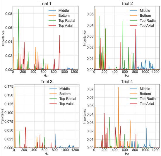
Figure 10.
4-Fold cross-validation for trials 1 to 4 of Gini importance considering 20 times averages using ERTs with optimal Linearity setting (n_estimators = 100, max_depth = None, min_samples_leaf = 2, min_samples_split = 10), and days.
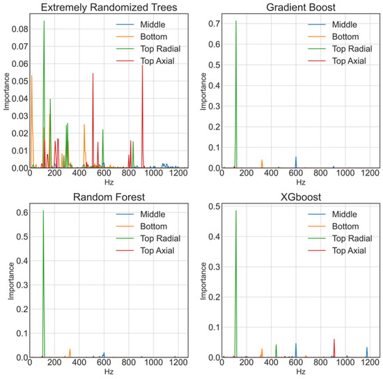
Figure 11.
Trial 1′s Gini importance of the 20 times average of using four different regressors using optimal RAE settings, with days.
3.5. Feature Selection of Gini Importance
The model in this study uses acceleration and motor current data to predict reactor health. In this case, Gini importance is used to reduce the size of the predicting model to analyze if it is helpful in prediction. Two methods are proposed for feature selection. Method 1 begins with training on an A/C dataset. After training, the ten most important features are chosen and combined with the motor current dataset to retrain. Finally, prediction outcomes are examined, which result in a similar RAE (Method 1: 0.291, Original: 0.307), but the averaged Linearity has greatly decreased (Method 1: 11.7, Original: 15.1). Figure 12 depicts the prediction results, where the color of each prediction point represents the health status (green for normal, orange for warning, and red for danger). The warning and danger status thresholds are manually given to be 40 and 20 days.
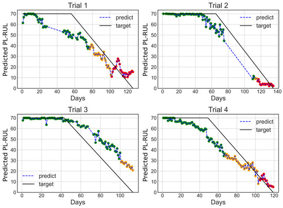
Figure 12.
4-Fold cross-validation results for trials 1 to 4 with days, trained on A/C dataset using Method 1 and ERTs regressor.
According to the above results, the high Gini importance features differ slightly between trials. We hypothesize that the features chosen are closely dependent on the training dataset. However, because the study aims to find universal features that can be used on any dataset in the system, a more complex method for selecting the critical features is proposed. To perform cross-validation, we train on three events and test on the fourth, as was previously mentioned. For Method 2, the training dataset is further split into three subsets, and separately trained. We then train a new model using the features that appear more than once in the top thirty Gini importance features of the training of the three subsets. Finally, the results are tested using the testing dataset. The two distinct feature selection processes are shown in Figure 13.
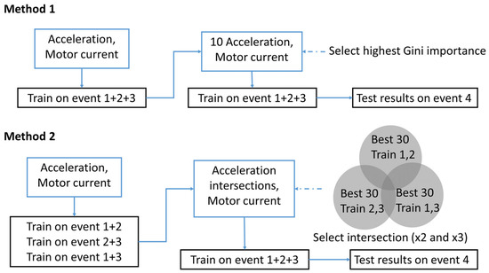
Figure 13.
Two different methods for feature selection using an example of Trial 4.
The predicted results utilizing features selected from Method 2 using the acceleration and motor dataset are shown in Figure 14. The color of each prediction point represents the health status (green for normal, orange for warning, and red for danger). The warning and danger status thresholds are manually given to be 40 and 20 days. The predicted results have an average RAE of 0.229, which is significantly less than 0.291 compared to Method 1 and is even better than the XGBoost regressor (A/C: 0.272), reaching the lowest RAE. The averaged Linearity is 11.6, which is similar to Method 1 results.
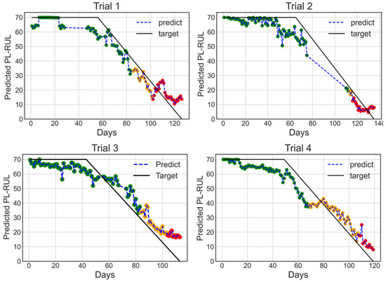
Figure 14.
4-fold cross-validation results with days for trials 1 to 4, Trained on features selected using Method 2 on A/C dataset using ERTs regressor. This result has the lowest averaged RAE.
The predicted results utilizing features selected from Method 2 using the acceleration dataset are shown in Figure 15, and the color of each prediction point represents the health status (green for normal, orange for warning, and red for danger). The warning and danger status thresholds are manually given to be 40 and 20 days. The predicted results have an average RAE of 0.253, which is slightly higher than 0.229 (A/C, Method 2). However, the average Linearity is 8.38, the smallest of all the results.
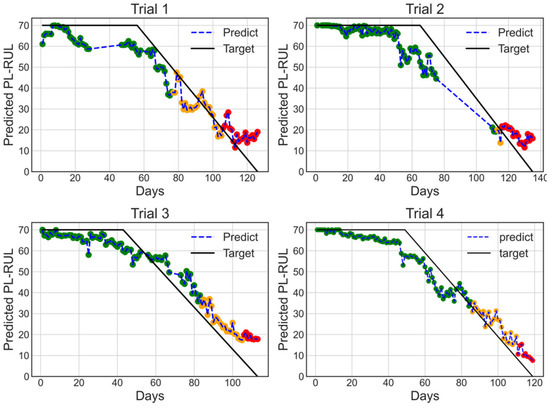
Figure 15.
4-fold cross-validation results with days for trials 1 to 4, trained on features selected using Method 2 on acceleration dataset having ERTs regressor with 100 estimators. This condition has the lowest averaged Linearity.
The response to the addition of the motor current dataset is intriguing. There is no significant difference in the results of the original method and feature selection Method 1 when adding the motor current dataset. However, when using Method 2, there are differences. Lower RAE can be achieved by adding motor currents, whereas lower Linearity can be achieved by removing motor currents. The decision tree regression process can explain this finding. The motor currents cut the decision tree in the motor currents dataset, so high-viscosity and low-viscosity conditions are dealt with separately. Better prediction and a lower RAE are the outcomes of these results. However, because fewer samples exist in each subcase, the prediction has a higher variance, resulting in higher Linearity. The Linearity could decrease if a larger dataset were provided.
4. Conclusions
This paper proposes a procedure for constructing a conditional health status prediction structure using a virtual health index, piecewise linear remaining useful life (PL-RUL), generated by machine learning regression methods trained on the acceleration and motor three-phased current (A/C) dataset for a supercritical ultra-high pressure chemical reactor bearing. The procedure remarks and findings of this research include:
- ■
- The Welch’s power spectrum density periodogram level is used to stifle strongly oscillating data and reduce the training data size by 16 times.
- ■
- We have successfully predicted the PL-RUL and health status using the Welch’s power spectrum density periodogram level and ERTs, which gives RAE and Linearity of 0.307 and 15.064, respectively.
- ■
- The analysis of the optimum selection of 70 days shows that our system has an optimum value, and PL-RUL is a better fit than RUL.
- ■
- We have performed grid search for hyperparameters tuning for seven commonly used regression algorithms. We discovered that ensemble trees algorithms have a smaller RAE than linear regression.
- ■
- Many ensemble trees algorithms, except for ERTs, have non-ideal staircase-like prediction behavior. We discovered that those with staircase-like behavior relied heavily on a few characteristic frequencies after investigating the Gini importance for each method. In contrast, the ERTs method has a large number of characteristic frequencies and hence exhibits linear behavior, making it a more suitable algorithm for this task.
- ■
- Two feature selection methods were proposed to improve prediction results. Method 1 can help improve the Linearity of the results from 15.1 to 11.7, whereas Method 2 can lower RAE from 0.307 to 0.229 in the acceleration and current combined (A/C) dataset and the Linearity from 15.1 to 8.4 in the acceleration (A) dataset.
- ■
- We have compared prediction with and without processing data (motor three-phase current) and discovered little difference between the two conditions before feature selection. However, following feature selection using Method 2, the prediction based on acceleration and motor current datasets has a lower RAE than the one without processing data. Still, the Linearity is higher, likely due to a lack of training samples.
We hope this paper would be a starting point for more researchers to notice and focus on applying machine learning predictive maintenance works for these ultra-high pressure systems. These works could greatly improve the efficiency of the reactor and reduce potential pollution and industrial safety hazards, driving us to a more sustainable future.
Author Contributions
Resources, S.-J.P.; data curation, S.-J.P.; methodology, S.-J.P.; validation, S.-J.P.; writing-original draft, S.-J.P. and M.-L.T.; investigation, M.-L.T.; software, M.-L.T.; visualization, M.-L.T.; project administration, C.-L.C.; writing-review & editing, C.-L.C.; supervision, P.T.L. and H.-Y.L. All authors have read and agreed to the published version of the manuscript.
Funding
This research was funded by the National Science and Technology Council, Taiwan (previously Ministry of Science and Technology, Taiwan), grant numbers MOST 110-2221-E-002-022 and MOST 111-2221-E-002-001.
Institutional Review Board Statement
Not applicable.
Informed Consent Statement
Not applicable.
Data Availability Statement
The data are not publicly available due to this information is confidential for anonymous company operations.
Conflicts of Interest
The authors declare no conflict of interest.
Notation
| Actual target for index | |
| Actual targets average | |
| Window energy correction factor | |
| Index of operating time | |
| Frequency band index | |
| Acceleration level of frequency band for sensor , dB | |
| Segments index | |
| Total segments | |
| Segmented, constant detrended, windowed, and zero-padded time series index | |
| Segment size | |
| Data length | |
| The predicted target for the index | |
| Periodogram of the mth block for sensor | |
| Inter-segment overlapping ratio | |
| Sensor index | |
| Welch’s power spectral density periodogram of the frequency band for the sensor | |
| Sampling frequency, Hz | |
| Current time, day | |
| End of use time of the bearing, day | |
| First predicting time, day | |
| Remaining useful life period, day | |
| The discrete sequence of the acceleration time-domain data for the sensor with index | |
| Zero-padded time series | |
| Hanning window function of length | |
| The mth segments of constant detrended, windowed, and zero-padded time series with index for sensor | |
| Frequency band with index , Hz |
Abbreviation
| A | Acceleration dataset |
| A/C | Accelerration plus motor current dataset |
| atm | Atmosphere |
| CNN | Convolution neural networks |
| DCS | Distributed control system |
| DFT | Discrete Fourier transform |
| ERTs | Extremely randomized trees |
| EVA | Ethylene-Vinyl Acetate |
| FFT | Fast Fourier Transform |
| FNN | Feed-forward neural network |
| KNN | K Nearest Neighbor |
| LCB | Long chain branch |
| LSTM | Long short-term memory |
| MI | Melting index |
| MSE | Mean square errors |
| MWD | Molecular weight distribution |
| PL-RUL | Piecewise linear remaining useful life |
| PSD | Power spectral density |
| RAE | Relative absolute error |
| RBF | Radial basis function |
| RF | Random Forest |
| RNN | Recurrent neural networks |
| RUL | Remaining useful life |
| SDGs | Sustainable Development Goals |
| SVM | Support vector machine |
| VA | Vinyl acetate |
| XGboost | eXtreme Gradient Boosting |
References
- Henderson, A. Ethylene-vinyl acetate (EVA) copolymers: A general review. IEEE Electr. Insul. Mag. 1993, 9, 30–38. [Google Scholar] [CrossRef]
- Sun, F.; Wang, G. Study on the thermal risk of the ethylene-vinyl acetate bulk copolymerization. Thermochim. Acta 2019, 671, 54–59. [Google Scholar] [CrossRef]
- Albert, J.; Luft, G. Runaway phenomena in the ethylene/vinylacetate copolymerization under high pressure. Chem. Eng. Process.-Process Intensif. 1998, 37, 55–59. [Google Scholar] [CrossRef]
- Turman, E.; Strasser, P.W. CFD modeling of LDPE autoclave reactor to reduce ethylene decomposition: Part 2 identifying and reducing contiguous hot spots. Chem. Eng. Sci. 2022, 257, 117722. [Google Scholar] [CrossRef]
- Brandolin, A.; Sarmoria, C.; Lótpez-Rodríguez, A.; Whiteley, K.S.; Del Amo Fernández, B. Prediction of molecular weight distributions by probability generating functions. Application to industrial autoclave reactors for high pressure polymerization of ethylene and ethylene-vinyl acetate. Polym. Eng. Sci. 2001, 41, 1413–1426. [Google Scholar] [CrossRef]
- Lee, H.-Y.; Yang, T.-H.; Chien, I.-L.; Huang, H.-P. Grade transition using dynamic neural networks for an industrial high-pressure ethylene–vinyl acetate (EVA) copolymerization process. Comput. Chem. Eng. 2009, 33, 1371–1378. [Google Scholar] [CrossRef]
- Sharma, P.; Sahoo, B.B. An ANFIS-RSM based modeling and multi-objective optimization of syngas powered dual-fuel engine. Int. J. Hydrogen Energy 2022, 47, 19298–19318. [Google Scholar] [CrossRef]
- Arena, S.; Florian, E.; Zennaro, I.; Orrù, P.; Sgarbossa, F. A novel decision support system for managing predictive maintenance strategies based on machine learning approaches. Saf. Sci. 2022, 146, 105529. [Google Scholar] [CrossRef]
- Hung, T.N.K.; Le, N.Q.K.; Le, N.H.; Van Tuan, L.; Nguyen, T.P.; Thi, C.; Kang, J.H. An AI-based Prediction Model for Drug-drug Interactions in Osteoporosis and Paget’s Diseases from SMILES. Mol. Inform. 2022, 41, e2100264. [Google Scholar] [CrossRef]
- Le, N.Q.K.; Do, D.T.; Nguyen, T.-T.; Le, Q.A. A sequence-based prediction of Kruppel-like factors proteins using XGBoost and optimized features. Gene 2021, 787, 145643. [Google Scholar] [CrossRef]
- Jin, S.; Sui, X.; Huang, X.; Wang, S.; Teodorescu, R.; Stroe, D.-I. Overview of Machine Learning Methods for Lithium-Ion Battery Remaining Useful Lifetime Prediction. Electronics 2021, 10, 3126. [Google Scholar]
- Lei, Y.; Li, N.; Guo, L.; Li, N.; Yan, T.; Lin, J. Machinery health prognostics: A systematic review from data acquisition to RUL prediction. Mech. Syst. Signal Process. 2018, 104, 799–834. [Google Scholar] [CrossRef]
- Moosavian, A.; Ahmadi, H.; Tabatabaeefar, A.; Khazaee, M. Comparison of Two Classifiers; K-Nearest Neighbor and Artificial Neural Network, for Fault Diagnosis on a Main Engine Journal-Bearing. Shock Vib. 2013, 20, 263–272. [Google Scholar] [CrossRef]
- Welch, P.D. The use of fast Fourier transform for the estimation of power spectra: A method based on time averaging over short, modified periodograms. IEEE Trans. Audio Electroacoust. 1967, 15, 70–73. [Google Scholar] [CrossRef]
- Long, Z.; Jun, Z. Rolling Bearing Fault Diagnosis Based on Ensemble Learning Model with WELCH Algorithm# br. Noise Vib. Control 2022, 42, 144. [Google Scholar]
- Jin, Z.; Han, Q.; Zhang, K.; Zhang, Y. An intelligent fault diagnosis method of rolling bearings based on Welch power spectrum transformation with radial basis function neural network. J. Vib. Control 2020, 26, 629–642. [Google Scholar] [CrossRef]
- Patil, S.; Phalle, V. Fault detection of anti-friction bearing using ensemble machine learning methods. Int. J. Eng. 2018, 31, 1972–1981. [Google Scholar]
- Rathore, M.S.; Harsha, S.P. Prognostic Analysis of High-Speed Cylindrical Roller Bearing Using Weibull Distribution and k-Nearest Neighbor. J. Nondestruct. Eval. Diagn. Progn. Eng. Syst. 2022, 5, 011005. [Google Scholar] [CrossRef]
- Xu, G.; Liu, M.; Jiang, Z.; Söffker, D.; Shen, W. Bearing fault diagnosis method based on deep convolutional neural network and random forest ensemble learning. Sensors 2019, 19, 1088. [Google Scholar] [CrossRef]
- Yang, Y.; Yu, D.; Cheng, J. A fault diagnosis approach for roller bearing based on IMF envelope spectrum and SVM. Measurement 2007, 40, 943–950. [Google Scholar] [CrossRef]
- Guo, L.; Li, N.; Jia, F.; Lei, Y.; Lin, J. A recurrent neural network based health indicator for remaining useful life prediction of bearings. Neurocomputing 2017, 240, 98–109. [Google Scholar] [CrossRef]
- Li, X.; Ding, Q.; Sun, J.-Q. Remaining useful life estimation in prognostics using deep convolution neural networks. Reliab. Eng. Syst. Saf. 2018, 172, 1–11. [Google Scholar] [CrossRef]
- Chen, Z.; Li, W. Multisensor feature fusion for bearing fault diagnosis using sparse autoencoder and deep belief network. IEEE Trans. Instrum. Meas. 2017, 66, 1693–1702. [Google Scholar] [CrossRef]
- Zheng, S.; Ristovski, K.; Farahat, A.; Gupta, C. Long short-term memory network for remaining useful life estimation. In Proceedings of the 2017 IEEE International Conference on Prognostics and Health Management (ICPHM), Dallas, TX, USA, 19–21 June 2017; IEEE: Piscataway, NJ, USA, 2017. [Google Scholar]
- Hu, C.; Youn, B.D.; Wang, P.; Yoon, J.T. Ensemble of data-driven prognostic algorithms for robust prediction of remaining useful life. Reliab. Eng. Syst. Saf. 2012, 103, 120–135. [Google Scholar] [CrossRef]
- Zhang, S.; Li, L.; Zhou, H.; Liu, H. Ensemble Learning Based Decision-Making Models on the Aero-Engine Bearing Fault Diagnosis. In Advances in Guidance, Navigation and Control; Springer: Berlin/Heidelberg, Germany, 2022; pp. 3829–3840. [Google Scholar]
- Zhou, H.; Cheng, L.; Teng, L.; Sun, H. Bearing Fault Diagnosis Based on RF-PCA-LSTM Model. In Proceedings of the 2021 2nd Information Communication Technologies Conference (ICTC), Nanjing, China, 7–9 May 2021; IEEE: Piscataway, NJ, USA, 2021. [Google Scholar]
- Patil, S.; Patil, A.; Phalle, V.M. Life prediction of bearing by using adaboost regressor. In Proceedings of the TRIBOINDIA-2018 An International Conference on Tribology, Mumbai, India, 13–15 December 2018. [Google Scholar]
- Shi, J.; Yu, T.; Goebel, K.; Wu, D. Remaining Useful Life Prediction of Bearings Using Ensemble Learning: The Impact of Diversity in Base Learners and Features. J. Comput. Inf. Sci. Eng. 2021, 21, 021004. [Google Scholar] [CrossRef]
- El-Thalji, I.; Jantunen, E. Dynamic modelling of wear evolution in rolling bearings. Tribol. Int. 2015, 84, 90–99. [Google Scholar] [CrossRef]
- Ramasso, E. Investigating computational geometry for failure prognostics in presence of imprecise health indicator: Results and comparisons on c-mapss datasets. In Proceedings of the PHM Society European Conference, Nantes, France, 8–10 July 2014. [Google Scholar]
- Heimes, F.O. Recurrent neural networks for remaining useful life estimation. In Proceedings of the 2008 International Conference on Prognostics and Health Management, Denver, CO, USA, 6–9 October 2008; IEEE: Piscataway, NJ, USA, 2008. [Google Scholar]
- Hong, C.-C.; Huang, S.-Y.; Shieh, J.; Chen, S.-H. Enhanced Piezoelectricity of Nanoimprinted Sub-20 nm Poly(vinylidene fluoride–trifluoroethylene) Copolymer Nanograss. Macromolecules 2012, 45, 1580–1586. [Google Scholar] [CrossRef]
- Kim, T.; Park, C.; Samuel, E.P.; Kim, Y.I.; An, S.; Yoon, S.S. Wearable sensors and supercapacitors using electroplated-Ni/ZnO antibacterial fabric. J. Mater. Sci. Technol. 2022, 100, 254–264. [Google Scholar] [CrossRef]
- Zhang, X.; Liu, Z.; Wang, J.; Wang, J. Time–frequency analysis for bearing fault diagnosis using multiple Q-factor Gabor wavelets. ISA Trans. 2019, 87, 225–234. [Google Scholar] [CrossRef]
- Wu, B.; Li, W.; Qiu, M. Remaining Useful Life Prediction of Bearing with Vibration Signals Based on a Novel Indicator. Shock Vib. 2017, 2017, 8927937. [Google Scholar] [CrossRef]
- Rahi, P.K.; Mehra, R. Analysis of power spectrum estimation using welch method for various window techniques. Int. J. Emerg. Technol. Eng. 2014, 2, 106–109. [Google Scholar]
- Pedregosa, F.; Varoquaux, G.; Gramfort, A.; Michel, V.; Thirion, B.; Grisel, O.; Blondel, M.; Prettenhofer, P.; Weiss, R.; Dubourg, V.; et al. Scikit-learn: Machine learning in Python. J. Mach. Learn. Res. 2011, 12, 2825–2830. [Google Scholar]
- Geurts, P.; Ernst, D.; Wehenkel, L. Extremely randomized trees. Mach. Learn. 2006, 63, 3–42. [Google Scholar] [CrossRef]
- Breiman, L. Random forests. Mach. Learn. 2001, 45, 5–32. [Google Scholar] [CrossRef]
- Drucker, H. Improving regressors using boosting techniques. In Proceedings of the ICML, Nashville, TN, USA, 8–12 July 1997. [Google Scholar]
- Friedman, J.H. Greedy function approximation: A gradient boosting machine. Ann. Stat. 2001, 29, 1189–1232. [Google Scholar] [CrossRef]
- Chen, T.; Guestrin, C. Xgboost: A scalable tree boosting system. In Proceedings of the 22nd ACM SIGKDD International Conference on Knowledge Discovery and Data Mining, San Francisco, CA, USA, 13–17 August 2016. [Google Scholar]
Disclaimer/Publisher’s Note: The statements, opinions and data contained in all publications are solely those of the individual author(s) and contributor(s) and not of MDPI and/or the editor(s). MDPI and/or the editor(s) disclaim responsibility for any injury to people or property resulting from any ideas, methods, instructions or products referred to in the content. |
© 2023 by the authors. Licensee MDPI, Basel, Switzerland. This article is an open access article distributed under the terms and conditions of the Creative Commons Attribution (CC BY) license (https://creativecommons.org/licenses/by/4.0/).