A Service Recommendation System Based on Dynamic User Groups and Reinforcement Learning

Abstract

Recently, advancements in machine-learning technology have enabled platforms such as short video applications and e-commerce websites to accurately predict user behavior and cater to their interests. However, the limited nature of user data may compromise the accuracy of these recommendation systems. To address personalized recommendation challenges and adapt to changes in user preferences, reinforcement-learning algorithms have been developed. These algorithms strike a balance between exploring new items and exploiting existing ones, thereby enhancing recommendation accuracy. Nevertheless, the cold-start problem and data sparsity continue to impede the development of these recommendation systems. Hence, we proposed a joint-training algorithm that combined deep reinforcement learning with dynamic user groups. The goal was to capture user preferences for precise recommendations while addressing the challenges of data sparsity and cold-start. We used embedding layers to capture representations and make decisions before the reinforcement-learning process, executing this approach cyclically. Through this method, we dynamically obtained more accurate user and item representations and provide precise recommendations. Additionally, to address data sparsity, we introduced a dynamic user grouping algorithm that collectively enhanced the recommendations using group parameters. We evaluated our model using movie-rating and e-commerce datasets. As compared to other baseline algorithms, our algorithm not only improved recommendation accuracy but also enhanced diversity by uncovering recommendations across more categories.

1. Introduction

Traditional recommendation algorithms have provided significant benefits to websites and applications that use recommendation systems. They have directly or indirectly contributed to the success of various service recommendation systems. However, recommendation systems themselves have faced several challenges that have hindered their development, leading to instability and low recommendation satisfaction during the initial stages of system operation. Researchers have tackled these issues using various methods. Singh et al. proposed a model that leveraged interactions among similar users, aggregating users’ purchase behavior as feedback to improve accuracy [1]. However, data sparsity has often resulted in insufficient data for training, and reinforcement learning, as an algorithm capable of obtaining feedback in real time, had frequently been applied to recommendation systems to enhance accuracy. Zhang et al. studied a fusion model of deep learning and reinforcement learning in order to establish a ranking framework that could effectively address data sparsity [2]. Other studies improved recommendation performance by incorporating users’ expected behaviors as feedback [3]. Some researchers have effectively used contextual features of user–object interactions to guide the selection of the next action. Similarly, in recent years, the popular multi-armed-bandit algorithms utilized contextual features as input, employing upper-confidence-interval algorithms to select the next action. Reinforcement learning has been used to maximize interests, enabling the discovery of the best strategy, and through experimentation, learning how to select the best arms for maximizing benefits [4,5,6]. When choosing the value-determining function, each experimenter must make selections based on unique characteristics and data science to achieve the highest click-through rate and utility.

However, despite the emergence of reinforcement learning allowing recommendation systems to maintain long-term learning states, the cold-start problem has persisted across various domains in recommendation systems, a consideration that our experiments also considered. The utilization of shared user-group parameters proved effective in alleviating this issue. When providing recommendations for individual users, we employed shared user-group parameters to mitigate the problem of overly specific preferences for a single user. To address the cold-start issues, users utilized features exhibiting similar preferences for the next recommendation in the group. In subsequent rounds of recommendations, this interesting point should not have to be consistently emphasized; instead, it should gradually diminish over time and with an increasing number of recommendation rounds, considering that user interests also evolve over time [7]. Therefore, our approach involved modeling the changing interests of users over time and accounting for the time-varying characteristics of user interest points.

After making recommendations, we could use these preferences to shape features that users were likely to have, even if it was not a perfect match. This was important because, during the early stages of user registration, predicting user needs accurately was challenging without sufficient data. Before users signed up, following the approach of He et al., we processed the available information [8]. We trained a neural model to help predict the probability of each action. In future recommendations, adapting to the evolving interests of users could be achieved through timely feedback, enabling dynamic recommendations.

When obtaining representations for users and items, some researchers has used pre-training methods to acquire more accurate prior probabilities for items [9,10]. Pre-training involves constructing initial features of the users and the items based on existing datasets and utilizing these features directly in subsequent recommendations. However, as user preferences may frequently change over time or due to other influencing factors, this approach had often led to sub-optimal results. In such cases, pre-constructed features had to be adjusted in some way to accommodate changes in the recommended probabilities caused by shifts in user preferences and tastes. Additionally, focusing solely on individual users or items could significantly increase the cost of recommendation systems, especially when there was insufficient interaction data available. Data sparsity and cold-start issues had hindered improvements in recommendation accuracy [4,11].

In this study, we proposed a joint-training algorithm, combining deep reinforcement learning with dynamic user clusters. As shown in Figure 1, this solution aimed to tackle the challenge of accurate representation and leveraged an enhanced Thompson sampling algorithm. The system used both rating data and preference information collected from sensors like GPS (Global Positioning System), image sensors, and biometric sensors, and input them into a database. After integrating the data, we used deep learning to obtain meaningful representations. We simultaneously updated three components: user-item embedding layers, user clusters, and reinforcement-learning back-propagation. By utilizing updates from these three components, we smoothly integrated the training of deep learning and reinforcement learning.

Figure 1. Data source and general operation process.

In the initial phase, we acquired preliminary user and item information, as well as group items, based on a scoring mechanism. In the stable phase, we continuously modified the numerical values and parameters of the three components to obtain precise user and item representations that were more conducive to recommendations.

Our specific contributions were as follows:

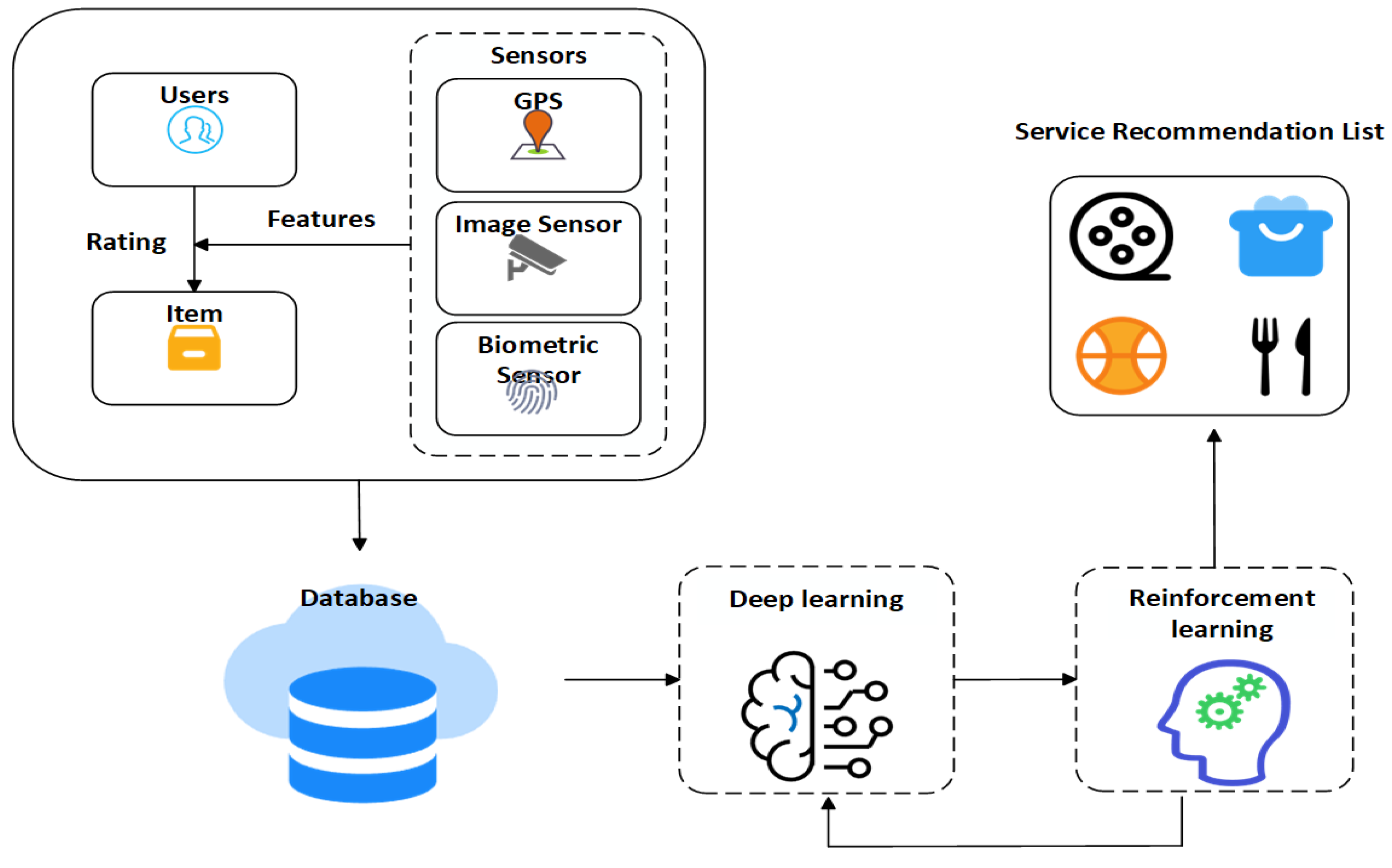
• We proposed a joint-training method using deep reinforcement learning and dynamic user grouping to address issues related to changing user preferences and data sparsity.
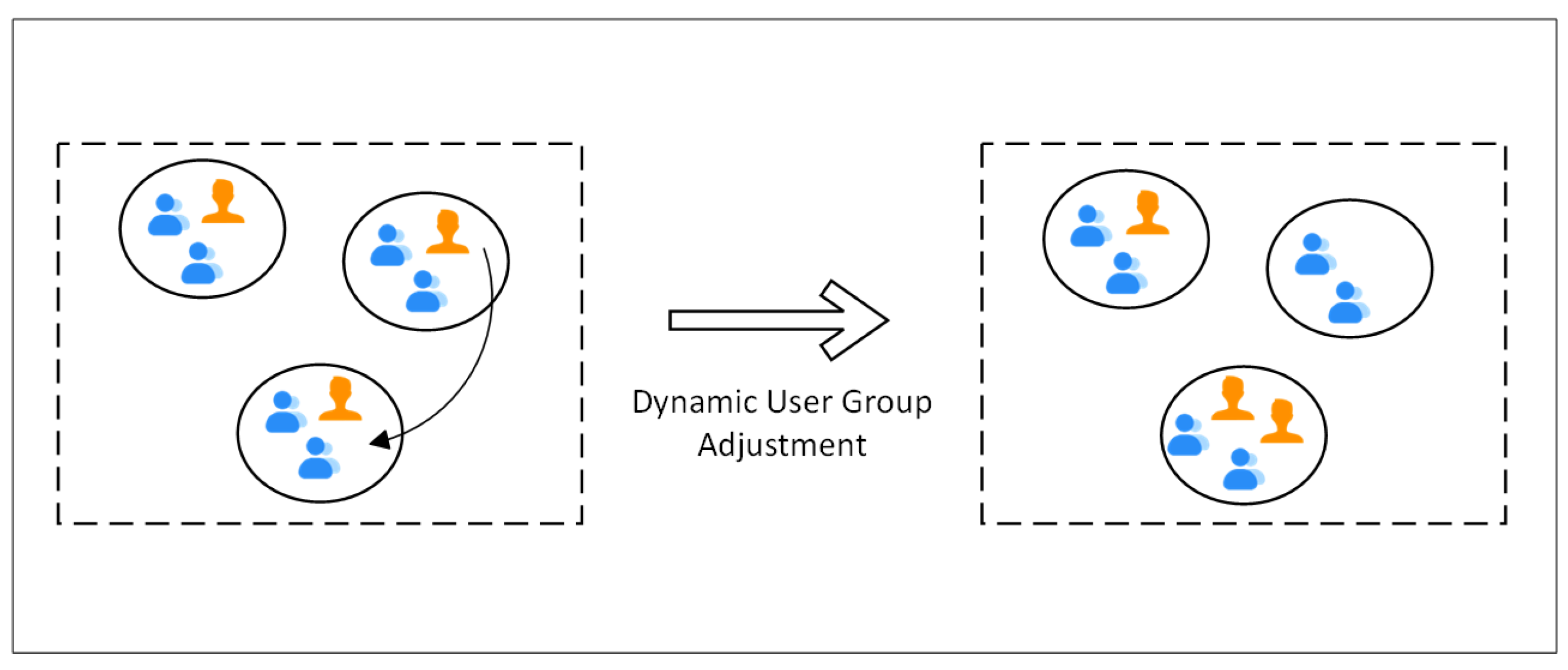
• We introduced a user-grouping mechanism that classified users based on project features. By aggregating users through shared parameters, this approach effectively alleviated challenges posed by sparse data and cold-start problems.
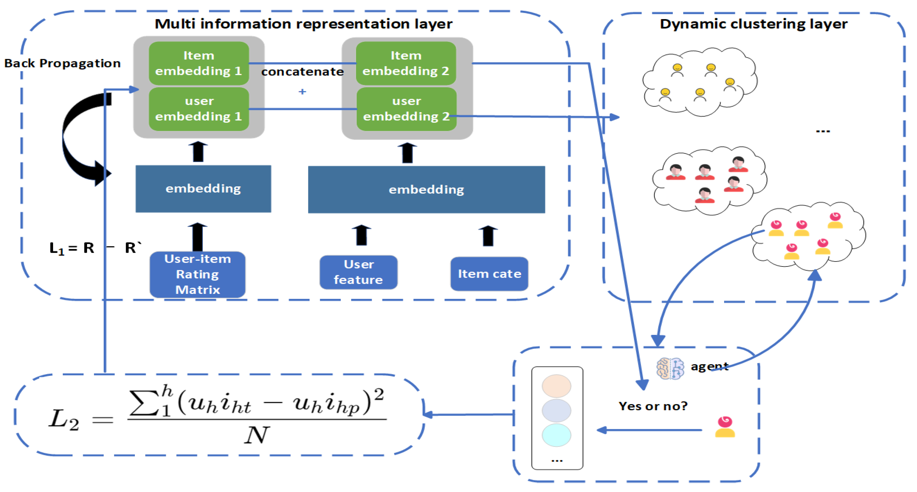
• The proposed joint-training algorithm combined deep learning and reinforcement learning. By concurrently operating between embedding layers and the decision layer in reinforcement learning, it captured users’ evolving preferences and provided optimal recommendations based on current user preferences.
• The experimental results on large datasets, such as MovieLens and Amazon, demonstrated a significant performance improvement, as compared to baseline algorithms. The model particularly excelled at mitigating cold-start and data-sparsity challenges. Additionally, its predictive accuracy surpassed that of baseline algorithms.

2. Related Work

In this section, algorithms and previous research relevant to our work are reviewed, including the matrix factorization algorithms we employed, the clustering bandit problem, the concept of user-based collaborative filtering, and attention mechanisms. These algorithms and concepts corresponded to different aspects of our study.

2.1. Matrix Factorization

Matrix factorization (MF) models are widely applied in machine-learning and recommendation systems. Recently, many MF models have been studied, aiming to decompose a large matrix into two or more smaller matrices in order to extract valuable information. A common approach has been to combine matrix factorization with other methods to create recommendation models. For example, NeuMF integrated traditional matrix methods with neural networks [12]. By using a multi-layer neural-network and matrix techniques, it captured interactions between users and items, enhancing NeuMF’s ability to model complex user–item relationships and provided more accurate personalized recommendations. BPR-MF employed a Bayesian framework specifically designed for handling implicit feedback data [13]. It learned user and item embeddings by maximizing ranking probabilities. This method was highly effective for personalized recommendations by handling implicit relationships between users and items, thereby elevating the level of personalization in recommendations. Guo et al. proposed the DeepFM model to address click-through-rate prediction problems by combining neural networks and factorization machines [14]. DeepFM could simultaneously capture low-level and high-level feature interactions, performing well in click-through-rate prediction tasks. It leveraged the powerful representation capabilities of neural networks, thus improving the accuracy of click-through-rate predictions. Most of the mentioned algorithms combined matrix factorization with other techniques to achieve the ultimate goal of recommendations, rather than solely relying on matrix factorization.

Considering existing matrix factorization algorithms, we believed that solely using matrix factorization algorithms showed excellent performance in some recommendation scenarios. Matrix factorization algorithms often needed to be combined with other algorithms to address the cold-start and data-sparsity issues and achieve optimal recommendation results. Therefore, by drawing inspiration from these works, we incorporated their ideas into our study to design our subsequent experiments. Furthermore, many matrix decompositions relied on abundant feature data, which could negatively impact the precision of the recommendation outcomes when the information was scarce. As a result, it was necessary to integrate these algorithmic concepts and devise new methods to alleviate data sparsity.

2.2. Contextual Multi-Armed Bandit Algorithm

This algorithm is distinctive in that it considers contextual information from the environment to intelligently select arms. Specifically, it employs methods like knowledge-graph embeddings to acquire contextual information about users and items. By taking into account these contextual details, the algorithm can better adapt to different environments and make wiser decisions.

In recent years, fundamental bandit algorithms have included the LinUCB [15] algorithm, Thompson [16] sampling, and emerging multi-armed bandit (MAB) algorithms based on deep reinforcement learning. For example, Gan et al. proposed a knowledge-enhanced contextual multi-armed bandit (CMAB) model that utilized knowledge-graph embeddings to obtain contextual information about users and items, ultimately treating items as arms for recommendations [17]. Other researchers have also attempted to build slot-machine models based on human emotions. For example, Huang et al. employed causal reasoning and introduced soft interventions to model arm-selection strategies [18]. This indicated they were trying to understand the interaction between user behavior and recommendation systems and use this as a foundation for devising recommendation strategies.

We drew inspiration from these experiments, as well, not only modeling items as arms in a slot machine but also considering emotions and deeper human thought processes, which were key to improving recommendation accuracy. We continuously updated user parameters based on feedback, ensuring that user preferences aligned as closely as possible with their current preferences.

2.3. User-Based Collaborative Filtering

User-based collaborative filtering (CF) has been a widely utilized approach in recommendation systems [19]. In this approach, the system identified similar users based on their item ratings and generated recommendations for the active users according to the preferences of similar users. Several similarity metrics have been proposed to measure the similarity between users, such as cosine similarity, Pearson’s correlation coefficient, and the Jaccard coefficient [20,21,22]. These metrics calculate user similarity by comparing their item ratings and have been used to construct similarity matrices representing the relationships among all pairs of users.

User-based CF has been successfully applied in various domains, like e-commerce, music, and social media. For example, Amazon.com used a user-based CF algorithm to recommend products to customers based on their purchase history and ratings [23]. New users were shown popular recommendations based on the preferences of other users, assuming their tastes aligned with the majority.

Zhao et al. focused on improving accuracy by enhancing user similarity metrics and neighborhood-selection methods to precisely capture preference relationships among users [24]. However, user-based CF had limitations, such as the cold-start problem for new users and the sparsity problem for users with few ratings. The cold-start problem occurred when a new user signed up but had not rated or expressed any preferences. In such cases, the system lacked information about the user’s preferences, hindering accurate recommendations. The sparsity problem occurred when users provided few ratings, making it challenging to identify similar users and generate accurate recommendations.

To address these challenges, various enhancement techniques have been proposed. A common technique has been neighborhood selection, involving the selection of a group of similar users to generate recommendations for the active user [25]. These techniques have successfully improved the performance of user-based CF, especially in scenarios with sparse data or a large user base.

These collaborative user-based filtering algorithms have provided us with powerful inspiration. By leveraging these fundamental algorithms, we could maximize the exploration and the utilization of user and item information, effectively alleviating data sparsity and cold-start issues. The necessary pre-training could overlook changes in user interests. Therefore, inspired by the collaborative filtering approach, we combined it with other methods to capture the evolving preferences of users.

2.4. The Attention Mechanism

The attention mechanism evaluated item features from various perspectives to emphasize those relevant to the recommendation task. Consequently, for each item, the attention mechanism adjusted its contribution in order to generate prior probabilities based on the importance of its features. This empowered the multi-armed bandit (MAB) algorithm to consider features holding higher informational value, enabling a more precise selection of optimal choices during the recommendation process.

Chen et al. proposed a collaborative filtering method using attention mechanisms and by considering different components of multimedia items [26]. This approach evaluated a user’s interest in various components of items, improving the effectiveness of multimedia recommendations. For example, Jin et al. designed an algorithm where attention mechanisms were used to extract key features from infrared images. By introducing channel attention and pixel attention, the network could focus on the more crucial parts of the task, enhancing overall visual quality. Li adopted attention mechanisms and short-term memory networks, contributing to better-capturing user interests and learning trajectories, thereby improving recommendation accuracy [27]. Wang et al. developed an algorithm that incorporated both dynamic attention-mechanism-based user-preference modeling and DL-based matching-score prediction [28]. The model integrated an attention mechanism to more effectively capture user preferences for subsequent operations. These mechanisms made the network more adaptive, enabling it to better handle diverse input scenarios. Inspired by these approaches, we designed a process for assigning attention values based on input.

3. Preliminaries

Following the reinforcement-learning (RL) paradigm [29], we treated the RL component as a multi-armed bandit problem. In the context of top-k recommendations, each item group was treated as an arm. The agent explored all arms based on their values and selected the arm with the maximum value. Subsections describe the methods employed in the reinforcement-learning part of this study.

3.1. Agent

In the design of our model, our primary objective was to guide the agent toward making choices that maximized its overall returns. We aimed for the agent to interact in various environments, learn, and optimize its decision-making strategy so that it could make decisions that could significantly increase returns when faced with diverse scenarios. Throughout this process, we focused on the adaptability of the agent’s decisions in different environments and how reinforcement-learning methods could enable it to choose actions more flexibly when encountering challenges. Through our model, we hoped the agent could learn a decision-making strategy that could perform optimally across a variety of situations.

3.2. States

Characterizing the current context of the environment involved defining a state, which was a detailed description of the environment reflecting the present location, condition, and situation where the agent was positioned. This state was influenced by the actions undertaken by the agent, as they led to changes in the environment. Specifically, in the context of our scenario, each element within the set represented a list of recommendations. The state at any given moment in time could be expressed as follows:

$$A_u=(a_{u1},a_{u2},a_{u3},\dots )$$

(1)

Here, $A_u$ symbolizes the state for a particular user u, and $a_{u1},a_{u2},a_{u3},\dots$ denotes the specific recommendations associated with that user at that specific moment. This state captures the dynamic nature of the environment, where alterations in the agent’s actions contribute to the evolution of the state, subsequently influencing the recommendations provided to the user.

3.3. Actions

In reinforcement learning, an agent can perform actions. The agent influences the environment by selecting actions. The selection of an action is the result of the agent’s policy decision in a particular state. At each moment, the system selects an action representing an arm, groups all items in the candidate pool based on the user’s preferences, and generates a recommendation list using a classifier, as follows:

$$a_u=(x_1,x_2,x_3\dots )$$

(2)

where $a_u$ is the set of candidate lists for user u.

3.4. Rewards

In our model, $x_{t,a}$ refers to the feature vector obtained by the user at time t after taking action a and pulling the arm, commonly known as the reward. This reward vector encompassed information about the changes in the environment state after the user interacted with it, serving as a crucial factor for evaluating the effectiveness of the agent’s actions.

More specifically, the reward vector $x_{t,a}$ could include a series of features reflecting the user’s preferences, behavioral history, and feedback from the environment after executing a particular action. Analyzing the reward vector allowed a deeper understanding of the outcomes of user–system interactions, guiding the learning process of the agent and optimizing recommendation strategies. In the framework of reinforcement learning, acquiring rewards was a critical step for the agent’s learning, as it reflected the contribution of user behavior to the system’s performance and provided essential information for the agent to make informed decisions in subsequent steps.

4. Proposed Method

4.1. Overview

Our problem could be divided into several main parts, including the multi-information representation module, the dynamic clustering module, the multi-level item-filtering module based on ratings, and the joint-training module. We abbreviated our model as DJT-RS and use this acronym throughout the rest of the text for reference, as shown in Figure 2. The overall implementation process is shown in Algorithm 1. Firstly, we split the problem by using a rating matrix and enhancing singular value decomposition to obtain user and item feature vectors [30]. Once we had these feature vectors, we used the nearest-neighbor algorithm to cluster users with similar preferences together, which was the role of the smart user-group module. This allowed users to spread information within the community, addressing the cold-start and data-sparsity issues. It was worth noting that when user embeddings changed, their preferences changed accordingly, leading to adjustments in the user groups. For each user U, we categorized items into several categories, forming “super arms”. Then, based on a selection strategy, we chose the most promising “arm”. During this process, we utilized back-propagation from the deep-learning and feedback values from the reinforcement learning for joint training. Based on the feedback, we adjusted user feature vectors, refined user groups, and repeated this process to achieve personalized recommendations.

Figure 2. DJT-RS Comprehensive Fact Sheet.

In the given context, $r_{ui}$ indicates the rating provided by user U to item I, ${\widehat{y}}_{ui}$ denotes the predicted rating by user U for item I, and U and I refer to the embeddings of the users and the items, respectively. The parameter $\rho$ is a regularization parameter that helps to control the model’s complexity.

Algorithm 1 Dynamic User Groups and Reinforcement Learning

Input: Rating data and contextual data. Output: Recommend list Data organization and data cleaning. for  $t=1,2,3,\dots$do     After utilizing data to obtain perceptual information in the embedding layer, acquire the average parameters $W_x$ for each user group.     Grouping of items based on current user preferences, Get all the arms $a=\mathrm{cate}\left(\right)$     The largest arm $i^{*}=arg{max}_{i\in \mathfrak{F}}\left(x_{t,a}+\alpha \sqrt{x_{t,a}^T{\overline{W}}_{\mathsf{n}}^{-1}{x}_{t,a}log(1+t)}\right)$ is carried out according to the equation     Observe the difference between the true and predicted total loss (L1+L2) for back-propagation     After examining the final results, adjust the feature information in the embedding layer based on L1.     Observe the final results again and modify the user group average parameters $W_x$ based on L2.     Adjust the user cluster where u belongs to     Move u from n1 to n2 end for

4.2. Multi-Information Representation

To make the raw data more informative, we introduced basic embedding logic into the multi-information representation layer. Unlike just obtaining embeddings, here we also dynamically updated feature vectors in coordination with other modules.

In the multi-information representation layer, the rating matrix was primarily decomposed using singular value decomposition. As shown in Figure 3, it started with the matrix decomposition, followed by feeding it into an embedding layer to obtain prediction values. Then, iterative back-propagation using the mean-squared error was applied until convergence. The loss function was defined as follows:

$$\mathrm{Loss}=\sum _{(u,i)}{(r_{ui}-{\widehat{y}}_{ui})}^2+\lambda \left({\parallel U\parallel }_F^2+{\parallel I\parallel }_F^2\right),$$

(3)

Next, to enhance representation capabilities, we obtained high-dimensional feature vectors for users (such as age, gender, occupation, etc.). Then, we obtained embeddings representing item categories. In the first round of recommendations (training), the embedding vectors of the users and the item components were connected separately. At this point, the initial feature construction was complete. The next stage involved the following tasks.

Figure 3. Eigenvector aggregation method.

After obtaining the embedding vectors, we introduced a weight redistribution mechanism. We used the obtained user and item embedding vectors, expanded them into several dimensions, and then used softmax to determine the importance of each weight. We added these dimensions together and used the average to obtain the final interpretable item feature. Please note that the attention mechanism, due to its resource-intensive nature, was only processed once before the first round and did not involve loop operations in subsequent iterations. The formula for synthesizing the final feature values for each feature domain was as follows:

$$\frac{{\sum }_{i=1}^n{\alpha }_i{x}_i}{{\sum }_{i=1}^n{x}_i},$$

(4)

4.3. Dynamic Clustering

Once we had obtained all the user feature vectors, we performed k-means clustering [31], dividing users into several user clusters. Each cluster’s parameters were represented by the average of the user feature vector within that cluster. The real-time user grouping implemented dynamic updating. For the first round of clustering, we used the Euclidean distance, the input was the user feature vector, the closest users were closely linked together, and the parameter of each user was the user feature vector calculated earlier. Therefore, the average parameter of each user group was:

$$W_n=\frac{{\sum }_{i=1}^{i=m}{u}_i}{m},$$

(5)

where u is an integer less than 50 and m is the number of users in each group. This provided the parameters shared externally by each user group $W_n$ and the use of shared parameters to mitigate the problem of under-representation of parameters by individual users.

Then, during the recommendation decision-making process, we used a user’s own feature vector, along with the parameters of the cluster to which they belonged, for personalized recommendations.

As shown in Figure 4, after each recommendation and based on feedback received, we recalculated the distances between the user and each cluster to update their cluster assignment.

Figure 4. The user leaves the original group and moves to the nearest group.

Additionally, a user’s feature vector was updated after each recommendation, not only at the end of training. This allowed the system promptly capture users’ changing preferences for more accurate recommendations. At this point, the gradient descent algorithm was used to comprehensively update user and item embedding information. The update produced a loss function that we defined as L1, as follows:

$$L_1=\frac{1}{u\ast i}\sum _{i=1}^{u\ast i}{(y_i-{\widehat{y}}_i)}^2,$$

(6)

where $y_i$ is the real rating and ${\widehat{y}}_i$ is the predictive score of the model. At this point, the training was over, and we could derive a rich vector representation of users as well as items. It was worth noting that this portion of the trained vectors was used for user clustering and prior probability initialization, and the user and vector representations were also re-scaled based on the loss values of subsequent recommendations.

Once the updates were complete, the refreshed user feature vectors were incorporated into the smart user group module for further computations.

The second phase involved using the constructed user and item features for user grouping and item categorization. This approach had the advantage of mitigating data sparsity and cold-start issues, as well as enabling the creation of personalized recommendation lists from which users could choose, thereby improving the robustness and the accuracy of the recommendation system.

Then, the k-means clustering algorithm was employed to categorize all users into groups. The clustering process began by initializing k data centroids, followed by iterative “assignment”, “update”, and “repeat” operations, until completion. In the assignment phase, assuming that $p_i$ represents the feature vector of a data point, $q_i$ is the center of cluster j, and n is the dimensionality of the feature vector, the formula for assigning data point $p_i$ to the nearest cluster center $q_i$ based on the distance was as follows:

$$d(p_i,q_j)=\sqrt{\sum _{k=1}^n{(p_{i,k}-q_{j,k})}^2},$$

(7)

for each cluster j, calculate the mean vector of all data points within that cluster as the new cluster center:

$$q_j=\frac{1}{|C_j|}\sum _{p_i\in C_j}{p}_i$$

(8)

Then, in the iterative process, minimize the loss function, which was expressed as:

$$J=\sum _{i=1}^m\sum _{j=1}^K{w}_{i,j}d(p_i,q_j),$$

(9)

where m represents the number of data points; K represents the number of clusters; $w_{i,j}$ is an variable that equals 1 if data point $p_i$ belongs to cluster j, otherwise $w_{i,j}$ equals 0; and $d(p_i,q_j)$ represents the distance between data point $p_i$ and cluster center $q_i$. In this way, we ultimately obtained k clusters. It was worth noting that, to avoid performing clustering at each recommendation, this operation was only executed once, and the subsequent updates to the clustering were handled by our algorithm.

4.4. A Multi-Level Item-Filtering Module Based on Ratings

When it came to delivering services such as news recommendations, product recommendations, and advertising, they have often been presented in the form of lists. In designing our service system, we took this into consideration. Therefore, we created a filtering mechanism to better categorize items.

First, we gathered a group of highly-rated items and divided them based on the maximum list size. Then, for items with relatively even ratings, we categorized them based on different categories. We also considered the user’s previous feedback in recommendations. Next, for lower-rated items, we shuffled and placed them in a low-probability pool, where they could be randomly selected with a low probability. This was performed because there were still many niche preferences within the broader audience.

In the design, we first categorized the highly rated items with the following formula:

$$C_i=\frac{R_i}{max\left(R\right)},$$

(10)

where $C_i$ is the categorization score of the item i, $R_i$ is the rating of the item i, and $max\left(R\right)$ is the highest rating among all the items. The categorization ensured that the high-rated items had more weight in the recommendation list.

Considering user feedback, we introduced a user feedback score:

$$S_i=\theta ·R_i+(1-\theta )·F_i,$$

(11)

where $S_i$ is the score of the item i after considering the user’s feedback, $\theta$ is a parameter that weighs the rating and the feedback, and $F_i$ is the user’s previous feedback score. To increase the selection probability of low-rated items, we used the following formula:

$$P_i=\frac{\mathrm{BaseProbability}}{\mathrm{BaseProbability}+e^{-\beta ·R_i}},$$

(12)

where BaseProbability is the base selection probability and $\beta$ is a parameter that adjusts the degree of enhancement of the selection probability of low-rated items. This selection probability function ensured that the low-rated items had additional flexibility in their probability of being selected, making them more likely to appear in the recommendation list.

4.5. Joint Training

Considering the continuously changing user preferences and behaviors based on emotions, we not only introduce reinforcement-learning algorithms to maximize returns but also utilized the changes in the embedding vectors representing users and items as a reflection of evolving user preferences [32]. Therefore, before starting the training, we spent some time training the representation layer of the users and the items. When it quickly converged, we initiated the entire system. The benefit of this approach was that it provided relatively accurate prior probabilities for the operation of selecting arms in the reinforcement learning.

During system operation, we could start recommendations at any time. After users had made recommendations, the system would update user and item embedding vectors based on the recommendation results. Simultaneously, it adjusted the parameters for the users and the user groups in the reinforcement learning. This was carried out to achieve joint training.

First, we had Loss1, which was a classic mean-squared-error (MSE) loss function. Its task was to match the model’s predictions to real data (usually user ratings or clicks) to ensure that the model performed well in terms of basic predictive accuracy.

We then introduced Loss2, which was the essence of reinforcement learning. Loss2 was computed by comparing the model’s recommendation results with the user’s actual clicking behavior. Specifically, we observed the difference between the items actually clicked on by the user and the items predicted to be clicked on by the model. The difference between the model’s recommendations and the actual clicks was interpreted as an error in its recommendations. If the model’s recommendations were very similar to the actual clicks, the Loss2 value would be close to zero. However, if the recommendations were significantly different from the actual clicks, the Loss2 value would be a large positive number. This loss function has commonly been used in reinforcement learning for tasks that were driven by rewards. The formula for L2 is shown below, where h represents the number of recommended items.

$$L_2=\frac{{\sum }_1^h{(u_h{i}_{ht}-u_h{i}_{hp})}^2}{N},$$

(13)

The final total loss was the combination of Loss1 and Loss2. Our goal was to minimize the total loss. This optimization process was performed by back-propagation, in which the parameters of the model, including the embedding vectors of the users and the items, were updated. This optimization process not only focused on the predictive accuracy of the model but also considered the performance of the model in user interactions to provide more personalized and effective recommendations.

In rating prediction, we classified different item classes based on labels and used each class to characterize the externally exposed item-feature vectors, and in the recommendation, each item class was considered as an action, i.e., an arm, which was selected based on the following equation:

$$i^{*}={argmax}_{i\in \mathfrak{F}}\left(x_{t,a}+\alpha \sqrt{x_{t,a}^T{\overline{W}}_{\mathsf{n}}^{-1}{x}_{t,a}log(1+t)}\right),$$

(14)

where $i^{*}$ denotes the best action to be selected; argmax indicates that the action to be selected is to find the action that maximizes the following expression among the set of possible actions; $i\in \mathfrak{I}$ denotes the set of optional actions, usually representing different slot arms (actions) in a multi-arm slot problem; $x_{t,a}$ denotes the value of action a at time t, usually representing the reward or benefit of a slot arm at a given time-step; $\alpha$ is a hyper-parameter used to balance the importance between the weight vector and the action feature vector; ${\overline{W}}_{\mathsf{n}}^{-1}$ is the inverse matrix of ${\overline{W}}_{\mathsf{n}}$, the matrix of the user group in which the user is located, which is often used to represent the uncertainty of the action eigenvectors; and $log(1+t)$ is a logarithmic function over time-steps, which increases over time.

The goal of this formulation was to select the action $\widehat{x}$ that should be taken at each time-step t to maximize the value of the value function. This value function consisted of the actual reward value of the action $x_{t,a}$ and a correction term that took into account uncertainty according to the inverse matrix of the covariance matrix ${\overline{W}}_{\mathsf{n}}^{-1}$. According to the equation, as time t increased, the consideration of uncertainty gradually increased, which meant that the system would choose its actions more carefully to maximize long-term returns.

This type of strategy has commonly been used in reinforcement learning to solve multi-arm slot-machine problems, where different actions (slot machine arms) could have different reward distributions. The goal was to find a strategy that maximized the total cumulative reward while accounting for uncertainty. This type of problem could be found in numerous domains, including online advertising [33,34], automated control [35,36], etc.

5. Experimental Results and Evaluation

In this section, we provide a thorough explanation of our algorithm’s experimental process. We conducted our experiments using two popular datasets, namely the MovieLens movie-rating dataset and the Amazon e-commerce dataset. We discuss detailed information about the datasets we used and also compare our results with baseline algorithms in the following sections.

5.1. Experimental Setup

5.1.1. Datasets

In this section, we explain the experimental process of our algorithm in detail. For this experiment, we used two well-known datasets: the MovieLens dataset and the Amazon e-commerce dataset. The MovieLens dataset contained rating data, user features, and item-category information. After data cleaning, there were a total of 943 users, 1682 item records, and 100,000 rating data points. In the case of the Amazon dataset, we used a dataset related to clothing purchases, which included 158 users, 98 items, and 30,000 rating data points. We provide a detailed explanation of the baseline algorithms used for comparison in the following sections.

5.1.2. Evaluation Metrics

DJT-RS primarily employed four metrics for evaluation. In addition to the three fundamental metrics for the recommendation systems, we also incorporated diversity metrics to assess the model’s ability to adapt to cold-start scenarios and alleviate data sparsity.

In our experiments, accuracy was defined as the ratio of the number of correct predictions to the overall predictions, i.e.,

$$\mathrm{Precision}=\frac{\mathrm{True}\mathrm{Positives}}{\mathrm{True}\mathrm{Positives}+\mathrm{False}\mathrm{Positives}}$$

(15)

where $\mathrm{True}\mathrm{Positives}$ is the number of users correctly predicted to be interested in the users and $\mathrm{False}\mathrm{Positives}$ is the number of users that were incorrectly predicted to be interested.

Recall was defined as how many of all true-positive category samples were correctly predicted as positive by the model.

$$\mathrm{Recall}=\frac{\mathrm{True}\mathrm{Positives}}{\mathrm{True}\mathrm{Positives}+\mathrm{False}\mathrm{Negatives}},$$

(16)

where $\mathrm{True}\mathrm{Positives}$ is the number of users correctly predicted to be interested and $\mathrm{False}\mathrm{Negatives}$ is the number of users incorrectly predicted to be uninterested.

The F1-score was a reconciled average of accuracy and recall and provided a comprehensive performance metric. It was calculated using the following formula:

$$F1=2\times \frac{\mathrm{Precision}\times \mathrm{Recall}}{\mathrm{Precision}+\mathrm{Recall}}$$

(17)

The F1-score considered the trade-off between accuracy and recall. It ranged from 0 to 1, with higher scores indicating that the model performed better in balancing precision and recall.

Finally, we defined the diversity metrics with the following formula:

$$\mathrm{Diversity}=\frac{1}{\left|\mathrm{U}\right|}\sum _{u\in U}\frac{{\sigma }_{\mathrm{domains}}\left(R\left(u\right)\right)}{{\mu }_{\mathrm{domains}}\left(R\left(u\right)\right)},$$

(18)

where U is the set of users, $R\left(u\right)$ is the recommendation list of user u, ${\sigma }_{\mathrm{domains}}$ is the standard deviation of the number of items in different categories in the recommendation list, and ${\mu }_{\mathrm{domains}}$ is the average number of items in different categories. The diversity metric evaluated the adaptability of the recommendation system in a cold-start state, that is, the larger the metric, the better the diversity of the recommendation system, in terms of providing different categories of items.

5.1.3. Baselines

When making recommendations, we used a method similar to a slot machine. During the comparison process, we focused on training both deep learning and reinforcement learning together. We selected the following algorithms to determine their effectiveness for improving data-scarcity problems within the recommendation system by analyzing user behavior patterns.

• SVD [37]: SVD is a classic matrix factorization algorithm that decomposed the rating matrix into three matrices: the user matrix, the item matrix, and the singular value matrix.
• LFM [38]: LFM is a probability-based matrix factorization method that introduced latent variables (hidden factors) to model the relationships between users and items. By learning these latent factors, the model could make personalized recommendations. This was a probabilistic matrix factorization method that introduced latent variables (hidden factors) to model the relationships between users and items. By learning these latent factors, the model could make personalized recommendations.
• NCF [39]: Neural collaborative filtering is a recommendation system method that combined the characteristics of neural networks to enhance the recommendation algorithms and improve the accuracy of personalized recommendations. It utilized neural networks to capture the complex relationships between users and items, allowing for better predictions of user interest in items. Typically, this approach introduced neural network layers on top of collaborative filtering to enhance the recommendation precision and personalization.
• LinUCB [40]: LinUCB is an algorithm for multi-armed bandit problems. It was based on linear models and the concept of confidence intervals in order to make the best decisions within a limited time frame. The algorithm estimated potential rewards and uncertainties for each choice and selected the optimal action based on these estimates.
• TS [41]: Thompson sampling is a reinforcement-learning algorithm used in multi-armed bandit problems and recommendation systems. It made optimal choices based on Bayesian probability.

5.2. Comparison with Baseline Algorithms

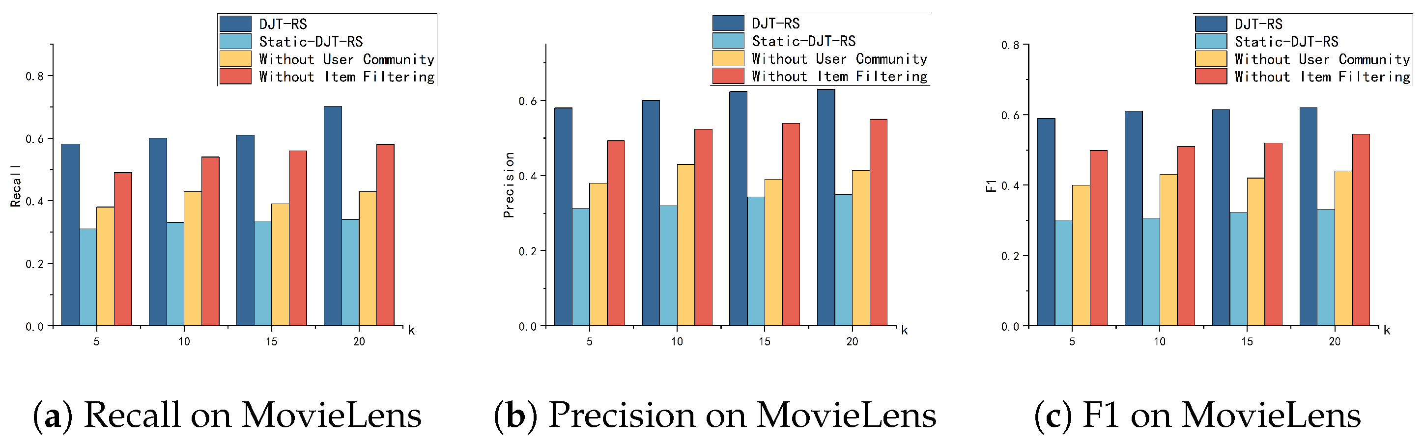
When comparing DJT-RS with other algorithms, we conducted top-k recommendations. The comparison results are shown in Table 1. Single recommendations often led to a significant drop in metrics. Here, we used three common metrics to compare various algorithms. Firstly, when k = 10, DJT-RS consistently outperformed other algorithms, regardless of which metric we examined. This was because it lacked sufficient reliable information and timely updates for recommendation results. It only performed one-time embedding. When facing sparse data, it often resulted in poor performance.

Table 1. Performance comparison on MovieLens and Amazon.

Datasets	Models	k = 10				k = 20				k = 30
		Recall	Precision	F1	Diversity	Recall	Precision	F1	Diversity	Recall	Precision	F1	Diversity
MovieLens	SVD	0.3902	0.3213	0.3538	0.2863	0.4354	0.4031	0.4186	0.2765	0.3954	0.3643	0.3793	0.3065
	LFM	0.4993	0.4214	0.4573	0.4658	0.4577	0.4003	0.4275	0.4895	0.5038	0.4357	0.4674	0.5268
	NCF	0.3894	0.3765	0.3829	0.4256	0.4038	0.3714	0.3872	0.4565	0.3953	0.3754	0.3852	0.6696
	LinUCB	0.5552	0.4662	0.5077	0.2659	0.6024	0.4721	0.5303	0.3596	0.5764	0.4921	0.5316	0.3985
	TS	0.5654	0.4532	0.5043	0.2685	0.5901	0.4601	0.5179	0.2985	0.6043	0.4945	0.5449	0.3698
	DJT-RS	0.6742	0.5364	0.5974	0.6859	0.7024	0.5572	0.6223	0.7596	0.6535	0.5313	0.5865	0.7776
Amazon	SVD	0.4353	0.3532	0.3902	0.3986	0.4662	0.4736	0.4699	0.4265	0.4276	0.3829	0.4043	0.4586
	LFM	0.5743	0.4564	0.5094	0.5463	0.4985	0.4355	0.4655	0.5796	0.5434	0.4875	0.5144	0.5593
	NCF	0.5432	0.4865	0.5139	0.5996	0.4576	0.4053	0.4301	0.6059	0.4363	0.3955	0.4148	0.6003
	LinUCB	0.6342	0.5334	0.5793	0.3236	0.6742	0.5623	0.6137	0.3363	0.5323	0.5231	0.5276	0.3238
	TS	0.6341	0.5962	0.6145	0.3696	0.6465	0.6041	0.6246	0.3889	0.5873	0.5437	0.5648	0.3826
	DJT-RS	0.6643	0.5923	0.6266	0.7652	0.6924	0.5963	0.6404	0.7966	0.6389	0.5212	0.5742	0.7652

For example, when k varied, the SVD algorithm had the highest metrics of recall 0.4354, precision 0.4031, and F1-score 0.4186. In the Amazon dataset, the corresponding recall, precision, and F1-score metrics were 0.4662, 0.4736, and 0.4699, which are relatively lower, as compared to other algorithms.

Comparatively, the LFM algorithm showed a slight improvement over the SVD algorithm. It could provide personalized lists for each user and utilized latent factors to fully explore implicit relationships in the data. However, it also lacked updates for the recommendation results, resulting in average performance.

Similarly, NCF was limited by data sparsity, which restricted its performance. In contrast, when using algorithms like Linucb and Thompson sampling, they could provide timely feedback on the recommendation results in order to guide the next recommendation. These two algorithms notably enhanced performance, as compared to the top three deep-learning algorithms.

Finally, at k = 10, the DJT-RS algorithm improved recall by 19% and 16% on MovieLens and Amazon, respectively. Precision increased by 15% on MovieLens, and F1-scores improved by 17% and 2% on MovieLens and Amazon, respectively. Similar improvements were observed at k = 20 and 30. For example, on MovieLens, at k = 20, the accuracy reached 0.5572, representing a 21% performance increase. This indicated that the algorithm’s accuracy gradually improved and captured user preferences through iterative trial and exploration. On Amazon, the accuracy was slightly lower than Thompson sampling due to the algorithm’s inclination to recommend more items to users, increasing recall while introducing more false positives and, thus, reducing accuracy. However, recall and F1-scores were consistently higher than Thompson sampling, demonstrating that our algorithm tended to strike a balance between exploration and exploitation and leaned towards trying new items for user recommendations. Additionally, in both datasets, when k = 20, the three metrics were generally higher than when k = 10 or k = 30, suggesting that recommending lists at k = 20 aligned more with user preferences and achieved the highest recommendation accuracy after balancing exploration and exploitation.

To assess the effectiveness of the algorithm for addressing data-sparsity and cold-start issues, we employed the standard-deviation diversity-detection method. The results indicated that DJT-RS, by utilizing a joint-training approach and providing timely feedback control for the recommended results, consistently exhibited superior diversity performance for any given value of k. This suggested that the DJT-RS method excelled at offering diverse items in the early stages of a recommendation system, mitigating biases towards popular items. It involved a wide range of item categories, ensuring better fairness for each item in the recommendation pool.

5.3. Ablation Study

5.3.1. Basic Ablation Study

During the analysis, we discussed the impact of various components of our model, such as the joint-training module, item-categorization module, and intelligent user-group module, on algorithm performance.

Firstly, we set k to different values in order to limit the number of recommended items. We split it into four values: k = 5, k = 10, k = 15, and k = 20. Then, we dissected the joint module, updating only the reinforcement learning without modifying the already trained user embeddings. This algorithm was referred to as static-DJT-RS, as shown in Figure 5 and Figure 6. If the embeddings had not been updated, system efficiency significantly decreased. This happened because user interests no longer adapted to changing preferences. Personalized recommendation efficiency also decreased, which was especially evident on the Amazon dataset, where user and item feature information were relatively scarce, as compared to the MovieLens dataset, leading to missing embedding-layer information and insufficient interest updates, resulting in a noticeable performance drop.

Figure 5. DJT-RS ablation experiment on the MovieLens dataset.

Figure 6. DJT-RS ablation experiment on the Amazon dataset.

Subsequently, we removed the intelligent user-group module, opting for recommendations based on individual user information without relying on their community. This algorithm was referred to as “without user community”. We observed that the achieved thresholds were not very high for any k-value. This was due to the user-group setting, effectively mitigating cold-start and data-sparsity issues.

Finally, removing the item-categorization module, referred to as “without item filtering”, resulted in a slight decline in system performance. In Figure 5, the effect was the same as the complete DJT-RS, but in other performance metrics, it still had a positive impact on recommendations. Possibly, in some recommendation rounds, the item-filtering module, based on ratings, effectively categorized items and filtered out popular items among users, leading to an improvement that may not have been significant.

In summary, the algorithm performed best when equipped with all three components: the joint-training module, intelligent user-group module, and item-categorization module. Each component enhanced user satisfaction to varying degrees, especially the joint-training module.

5.3.2. Diversity Comparison

To compare the DJT-RS algorithm with other baseline algorithms in terms of addressing data sparsity and overcoming cold-start challenges, we conducted top-k recommendations on the MovieLens dataset. We set k to 20 and performed tests on the first 100 users. All baseline algorithms were trained and tested from the same starting point. As shown in Figure 7, our algorithm exhibited a significant improvement in diversity, as compared to the other algorithms. This indicated that our algorithm could recommend items from a wider range of categories to users while maintaining stable increases in the accuracy and recall metrics. A higher diversity value implied a greater variety of recommended item categories, showcasing a higher proportion of exploration in the recommendations. This provided evidence that our algorithm could mitigate cold-start and data-sparsity issues, to some extent.

Figure 7. Comparison of diversity between DJT-RS and baseline algorithms.

6. Conclusions

Our experimental results indicated that, as compared to algorithms trained directly with deep learning for feature extraction, our joint-training approach was more conducive to capturing dynamically changing preferences among users. Unlike the multi-armed bandit algorithm, our input context was both interpretable and time-varying. User preferences evolve over time, and in the initial recommendation stage, our algorithm could quickly identify user points of interest, significantly reducing the cold-start time of the recommendation system. In summary, our proposed service recommendation system based on dynamic user groups and reinforcement learning was an effective recommendation system that could provide insights and inspiration for practical application scenarios. In the future, we will continue to explore ways to further enhance the efficiency and the accuracy of the algorithm in order to make more significant contributions to the development of recommendation systems.

References

1. Singh, J.; Sajid, M.; Yadav, C.S.; Singh, S.S.; Saini, M. A Novel Deep Neural-based Music Recommendation Method considering User and Song Data. In Proceedings of the 2022 6th International Conference on Trends in Electronics and Informatics (ICOEI), Tirunelveli, India, 28–30 April 2022; pp. 1–7. [Google Scholar]
2. Zha, D.; Feng, L.; Tan, Q.; Liu, Z.; Lai, K.H.; Bhushanam, B.; Tian, Y.; Kejariwal, A.; Hu, X. Dreamshard: Generalizable embedding table placement for recommender systems. Adv. Neural Inf. Process. Syst. 2022, 35, 15190–15203. [Google Scholar]
3. Intayoad, W.; Kamyod, C.; Temdee, P. Reinforcement learning based on contextual bandits for personalized online learning recommendation systems. Wirel. Pers. Commun. 2020, 115, 2917–2932. [Google Scholar] [CrossRef]
4. Sanz-Cruzado, J.; Castells, P.; López, E. A simple multi-armed nearest-neighbor bandit for interactive recommendation. In Proceedings of the 13th ACM Conference on Recommender Systems, Copenhagen, Denmark, 16–20 September 2019; pp. 358–362. [Google Scholar]
5. Elena, G.; Milos, K.; Eugene, I. Survey of multiarmed bandit algorithms applied to recommendation systems. Int. J. Open Inf. Technol. 2021, 9, 12–27. [Google Scholar]
6. Qin, L.; Chen, S.; Zhu, X. Contextual combinatorial bandit and its application on diversified online recommendation. In Proceedings of the 2014 SIAM International Conference on Data Mining, Philadelphia, PA, USA, 24–26 April 2014; pp. 461–469. [Google Scholar]
7. Jiang, J.; Jiang, Y. Leader-following consensus of linear time-varying multi-agent systems under fixed and switching topologies. Automatica 2020, 113, 108804. [Google Scholar] [CrossRef]
8. Li, S.; Lei, W.; Wu, Q.; He, X.; Jiang, P.; Chua, T.S. Seamlessly unifying attributes and items: Conversational recommendation for cold-start users. Acm Trans. Inf. Syst. (TOIS) 2021, 39, 1–29. [Google Scholar] [CrossRef]
9. Aldayel, M.; Al-Nafjan, A.; Al-Nuwaiser, W.M.; Alrehaili, G.; Alyahya, G. Collaborative Filtering-Based Recommendation Systems for Touristic Businesses, Attractions, and Destinations. Electronics 2023, 12, 4047. [Google Scholar] [CrossRef]
10. Lv, Z.; Tong, X. A Reinforcement Learning List Recommendation Model Fused with Graph Neural Networks. Electronics 2023, 12, 3748. [Google Scholar] [CrossRef]
11. Ahmadian, S.; Ahmadian, M.; Jalili, M. A deep learning based trust-and tag-aware recommender system. Neurocomputing 2022, 488, 557–571. [Google Scholar] [CrossRef]
12. Ahmadian, M.; Ahmadian, S.; Ahmadi, M. RDERL: Reliable deep ensemble reinforcement learning-based recommender system. Knowl.-Based Syst. 2023, 263, 110289. [Google Scholar] [CrossRef]
13. Rendle, S.; Freudenthaler, C.; Gantner, Z.; Schmidt-Thieme, L. BPR: Bayesian personalized ranking from implicit feedback. arXiv 2012, arXiv:1205.2618. [Google Scholar]
14. Guo, H.; Tang, R.; Ye, Y.; Li, Z.; He, X. DeepFM: A factorization-machine based neural network for CTR prediction. arXiv 2017, arXiv:1703.04247. [Google Scholar]
15. Semenov, A.; Rysz, M.; Pandey, G.; Xu, G. Diversity in news recommendations using contextual bandits. Expert Syst. Appl. 2022, 195, 116478. [Google Scholar] [CrossRef]
16. Kawale, J.; Bui, H.H.; Kveton, B.; Tran-Thanh, L.; Chawla, S. Efficient Thompson sampling for Online Matrix-Factorization Recommendation. In Proceedings of the Advances in Neural Information Processing Systems, Montreal, QC, Canada, 7–12 December 2015; Volume 28. [Google Scholar]
17. Gan, M.; Kwon, O.C. A knowledge-enhanced contextual bandit approach for personalized recommendation in dynamic domains. Knowl.-Based Syst. 2022, 251, 109158. [Google Scholar] [CrossRef]
18. Huang, W.; Zhang, L.; Wu, X. Achieving counterfactual fairness for causal bandit. Proc. AAAI Conf. Artif. Intell. 2022, 36, 6952–6959. [Google Scholar] [CrossRef]
19. Setiowati, S.; Adji, T.B.; Ardiyanto, I. Point of Interest (POI) Recommendation System using Implicit Feedback Based on K-Means+ Clustering and User-Based Collaborative Filtering. Comput. Eng. Appl. J. 2022, 11, 73–88. [Google Scholar] [CrossRef]
20. Yunanda, G.; Nurjanah, D.; Meliana, S. Recommendation system from microsoft news data using TF-IDF and cosine similarity methods. Build. Inform. Technol. Sci. (BITS) 2022, 4, 277–284. [Google Scholar] [CrossRef]
21. van den Heuvel, E.; Zhan, Z. Myths about linear and monotonic associations: Pearson’s r, Spearman’s ρ, and Kendall’s τ. Am. Stat. 2022, 76, 44–52. [Google Scholar] [CrossRef]
22. Jain, G.; Mahara, T.; Sharma, S.C.; Sangaiah, A.K. A cognitive similarity-based measure to enhance the performance of collaborative filtering-based recommendation system. IEEE Trans. Comput. Soc. Syst. 2022, 9, 1785–1793. [Google Scholar] [CrossRef]
23. Linden, G.; Smith, B.; York, J. Amazon.com recommendations: Item-to-item collaborative filtering. IEEE Internet Comput. 2003, 7, 76–80. [Google Scholar] [CrossRef]
24. Zhao, Z.D.; Shang, M.S. User-based collaborative-filtering recommendation algorithms on hadoop. In Proceedings of the 2010 Third International Conference on Knowledge Discovery and Data Mining, Phuket, Thailand, 9–10 January 2010; pp. 478–481. [Google Scholar]
25. Hsieh, F.S. Trust-based recommendation for shared mobility systems based on a discrete self-adaptive neighborhood search differential evolution algorithm. Electronics 2022, 11, 776. [Google Scholar] [CrossRef]
26. Chen, J.; Zhang, H.; He, X.; Nie, L.; Liu, W.; Chua, T.S. Attentive collaborative filtering: Multimedia recommendation with item-and component-level attention. In Proceedings of the 40th International ACM SIGIR conference on Research and Development in Information Retrieval, Tokyo, Japan, 7–11 August 2017; pp. 335–344. [Google Scholar]
27. Li, B. Optimisation of UCB algorithm based on cultural content orientation of film and television in the digital era. Int. J. Netw. Virtual Organ. 2023, 28, 265–280. [Google Scholar] [CrossRef]
28. Wang, R.; Wu, Z.; Lou, J.; Jiang, Y. Attention-based dynamic user modeling and deep collaborative filtering recommendation. Expert Syst. Appl. 2022, 188, 116036. [Google Scholar] [CrossRef]
29. Aramayo, N.; Schiappacasse, M.; Goic, M. A Multiarmed Bandit Approach for House Ads Recommendations. Mark. Sci. 2023, 42, 271–292. [Google Scholar] [CrossRef]
30. Al-Ajlan, A.; Alshareef, N. Recommender System for Arabic Content Using Sentiment Analysis of User Reviews. Electronics 2023, 12, 2785. [Google Scholar] [CrossRef]
31. Ikotun, A.M.; Ezugwu, A.E.; Abualigah, L.; Abuhaija, B.; Heming, J. K-means clustering algorithms: A comprehensive review, variants analysis, and advances in the era of big data. Inf. Sci. 2022, 622, 178–210. [Google Scholar] [CrossRef]
32. Dang, C.N.; Moreno-García, M.N.; Prieta, F.D. An approach to integrating sentiment analysis into recommender systems. Sensors 2021, 21, 5666. [Google Scholar] [CrossRef]
33. Naeem, M.; Rizvi, S.T.H.; Coronato, A. A gentle introduction to reinforcement learning and its application in different fields. IEEE Access 2020, 8, 209320–209344. [Google Scholar] [CrossRef]
34. Iacob, A.; Cautis, B.; Maniu, S. Contextual bandits for advertising campaigns: A diffusion-model independent approach. In Proceedings of the 2022 SIAM International Conference on Data Mining (SDM), Alexandria, VA, USA, 28–30 April 2022; pp. 513–521. [Google Scholar]
35. Ding, Q.; Kang, Y.; Liu, Y.W.; Lee, T.C.M.; Hsieh, C.J.; Sharpnack, J. Syndicated bandits: A framework for auto tuning hyper-parameters in contextual bandit algorithms. Adv. Neural Inf. Process. Syst. 2022, 35, 1170–1181. [Google Scholar]
36. London, B.; Joachims, T. Control Variate Diagnostics for Detecting Problems in Logged Bandit Feedback. 2022. Available online: https://www.amazon.science/publications/control-variate-diagnostics-for-detecting-problems-in-logged-bandit-feedback (accessed on 12 December 2023).
37. Colace, F.; Conte, D.; De Santo, M.; Lombardi, M.; Santaniello, D.; Valentino, C. A content-based recommendation approach based on singular value decomposition. Connect. Sci. 2022, 34, 2158–2176. [Google Scholar] [CrossRef]
38. Fang, H.; Bao, Y.; Zhang, J. Leveraging decomposed trust in probabilistic matrix factorization for effective recommendation. In Proceedings of the AAAI Conference on Artificial Intelligence, Quebec City, QC, Canada, 27–31 July 2014; Volume 28. [Google Scholar] [CrossRef]
39. He, X.; Liao, L.; Zhang, H.; Nie, L.; Hu, X.; Chua, T.S. Neural collaborative filtering. In Proceedings of the 26th International Conference on World Wide Web, Perth, Australia, 3–7 April 2017; pp. 173–182. [Google Scholar]
40. Shi, Q.; Xiao, F.; Pickard, D.; Chen, I.; Chen, L. Deep Neural Network with LinUCB: A Contextual Bandit Approach for Personalized Recommendation. In Proceedings of the Companion Proceedings of the ACM Web Conference 2023, Austin, TX, USA, 30 April–4 May 2023; pp. 778–782. [Google Scholar]
41. Agrawal, S.; Goyal, N. Analysis of thompson sampling for the multi-armed bandit problem. In Proceedings of the Conference on Learning Theory, Lyon, France, 29–31 October 2012; JMLR Workshop and Conference Proceedings. pp. 39.1–39.26. [Google Scholar]
Disclaimer/Publisher’s Note: The statements, opinions and data contained in all publications are solely those of the individual author(s) and contributor(s) and not of MDPI and/or the editor(s). MDPI and/or the editor(s) disclaim responsibility for any injury to people or property resulting from any ideas, methods, instructions or products referred to in the content.
Article Metrics
Citations
Article Access Statistics
Multiple requests from the same IP address are counted as one view.