Article

Enhancing Outdoor Moving Target Detection: Integrating Classical DSP with mmWave FMCW Radars in Dynamic Environments

by
Debjyoti Chowdhury
1,
Nikhitha Vikram Melige
2,3,*,
Biplab Pal
2,3 and
Aryya Gangopadhyay
2,3
1
Heritage Institute of Technology, Kolkata 700107, India
2
Department of Information Systems, University of Maryland Baltimore County, Baltimore, MD 21250, USA
3
Center for Real-Time Distributed Sensing and Autonomy, University of Maryland Baltimore County, Baltimore, MD 21250, USA
*
Author to whom correspondence should be addressed.
Electronics 2023, 12(24), 5030; https://doi.org/10.3390/electronics12245030
Submission received: 14 October 2023 / Revised: 8 December 2023 / Accepted: 14 December 2023 / Published: 16 December 2023
(This article belongs to the Special Issue Machine Learning for Radar and Communication Signal Processing)

Abstract

:
This paper introduces a computationally inexpensive technique for moving target detection in challenging outdoor environments using millimeter-wave (mmWave) frequency-modulated continuous-wave (FMCW) radars leveraging traditional signal processing methodologies. Conventional learning-based techniques for moving target detection suffer when there are variations in environmental conditions. Hence, the work described here leverages robust digital signal processing (DSP) methods, including wavelet transform, FIR filtering, and peak detection, to efficiently address variations in reflective data. The evaluation of this method is conducted in an outdoor environment, which includes obstructions like woods and trees, producing an accuracy score of 92.0% and precision of 91.5%. Notably, this approach outperforms deep learning methods when it comes to operating in changing environments that project extreme data variations.

1. Introduction

Radar technology plays a critical role in both civilian and military applications, employing electromagnetic waves to detect targets, regardless of weather conditions or time of day [1,2,3]. However, the complexity of real-world environments and the diversity of targets pose challenges in radar detection, potentially due to weaknesses in target returns [4,5,6]. To address these challenges, researchers worldwide are focusing on developing adaptive and resilient target identification techniques. A significant challenge in radar target identification lies in characterizing cluttered features using specific distribution models in dynamic and complex environments [7,8,9]. To overcome these challenges, radar systems increasingly incorporate self-learning, adapting, and self-optimizing processing capabilities. The advent of artificial intelligence technologies has provided valuable support for intelligent radar design. Deep learning, a branch of machine learning encompassing convolutional neural networks (CNNs) [10] and recurrent neural networks (RNNs) [11], has demonstrated remarkable capabilities in automatic feature learning and extraction, enabling tasks such as intelligent recognition of speech information and image segmentation [12]. Deep learning has also been successfully applied in radar, particularly for the intelligent detection and processing of high-resolution synthetic aperture radar (SAR) images [13]. However, these techniques often struggle when applied to environments that differ from those they were trained in, and they can also be computationally demanding. Traditional radar target identification methods are categorized based on processing domains: time domain, frequency domain, and time-frequency (TF) domain. While effective in many scenarios, traditional time-domain processing techniques, such as constant false-alarm rate (CFAR) detection [14] and coherent or non-coherent accumulation, face difficulties in dynamic and changing environments with non-Gaussian, non-stationary, and non-linear features. Frequency domain techniques, such as moving target indicator (MTI) and moving target detection (MTD), utilize Doppler information extracted through the Fourier transform [13]. Moving target detection (MTD) is a crucial task in various applications, ranging from conventional surveillance to autonomous driving. The increased adoption of mmWave Frequency Modulated Continuous Wave (FMCW) radars for MTD is driven by their advantages, including high resolution, broad operational range, and obstacle penetration. However, mmWave FMCW radars are susceptible to noise and interference in unconstrained environments. Conventional MTD algorithms for mmWave FMCW radars often rely on classical signal processing techniques like wavelet transforms, finite impulse response (FIR) filtering, and peak detection.
In response to these challenges, this paper introduces an innovative MTD approach specifically tailored for mmWave FMCW radars, intending to identify moving targets in areas with dense to medium foliage from a distance of 30 m to the radar. The proposed methodology integrates classical Digital Signal Processing (DSP) techniques with novel strategies, aiming to provide a holistic and robust approach to extreme data variations [15,16,17]. This integration leverages the strengths of both traditional signal processing and innovative methodologies, effectively addressing inherent limitations. The goal is to establish the applicability of classical signal processing in resource-limited practical scenarios and set a performance benchmark by comparing signal processing-based MTD with available deep learning-based techniques. Consequently, this research seeks to bridge the gap between classical signal processing and emerging deep learning techniques, fostering the development of more robust, practical, and efficient MTD solutions for mmWave FMCW radar systems, thereby advancing the state-of-the-art in radar-based sensing [18].
The key contributions of the work are as follows:
  • Development of computationally inexpensive MTD algorithm.
  • Tackle data variations in range-Doppler data through classical DSP techniques.
  • Develop a low-cost edge deployed radar-based MTD system
This paper is structured to provide a comprehensive understanding of the research. In Section 1, the introduction outlines the objectives and context for subsequent sections. Section 2 delves into the signal processing pipeline and presents a mathematical description of the mmWave radar’s range-Doppler data. This section elucidates the methodology and data processing intricacies. Section 3 covers experimental aspects, with Section 3.1 detailing the setup and configuration for data collection. Section 3.2 addresses performance parameters, and the comparative analysis with other techniques is given in Section 3.3. The concluding Section 4 summarizes the findings and insights derived from the research.

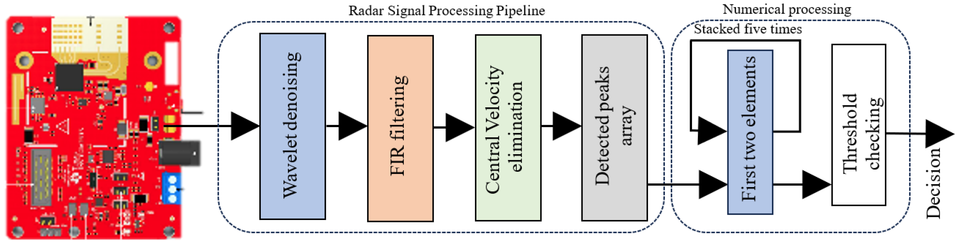
2. System Description

The experimental research utilizes the Texas Instruments AWR 1642 BOOST [19] radar, employing frequency-modulated continuous waves (FMCW or chirps) transmitted by the onboard Cortex®-R4F MCU. Chirp settings are configured for transmission, and RX antennas capture reflected signals. The onboard ADC converts analog IF signals to digital signals, providing object range information and velocity data based on phase differences. The digitized data are processed through a hardware accelerator (HWA) for 1D Fast Fourier Transform (range-FFT) to generate range-time maps. DSP C67x then performs 2D-FFT (velocity-FFT) on the maps to generate velocity-time maps. The first dimension of the FFT is the range dimension, and the second dimension is the Doppler dimension. An FMCW radar, as previously stated, generates a series of wideband chirp signals to illuminate the monitored area. The burst of N c up-chirps can be expressed at the TX antenna input terminals as Equation (1) [20].
S t x ( t ) = A t x n c = 0 N c 1 cos [ Ψ ( t ) ] t T c 2 n c T P R I T c
Here, A t x represents the signal amplitude, and Ψ ( t ) = 2 π ( f 0 t s + 0.5 μ t s 2 ) denotes the up-chirp phase. Here, T c is the duration of a single up-chirp, T P R I is the pulse repetition interval (PRI), and t s = t n c T P R I defines the fast-time, with t s restricted to the interval [ 0 , T c ] , where n c is the slow-time index. The parameters f 0 , μ = B / T c , and B represent the starting frequency, sweep rate, and bandwidth of the sweep, respectively. The function ( χ ) yields 1 when | χ | 1 / 2 and 0 otherwise. Between successive up-chirps, a recovery time, where T P R I > T c , is typically inserted. During this period, the frequency synthesizer resets to its initial state, and the relative echo signal is disregarded. The collection of chirps, referred to as a frame, has a duration of T C P I = T P R I N c , where C P I stands for the coherent processing interval. A specific interval is commonly inserted before the next burst, resulting in a frame period T f that exceeds T C P I .
q I F ( n s , n c ) = A I F e j 2 π ( f b T s n s f D T T R I n c ) with n s = 0 , , N s 1 , n c = 0 , , N c 1
where, A I F is proportional to the strength of the received echo, denoted as A r x , and T s is the sampling period, several parameters are involved. The Doppler shift, given by f D = 2 v r / λ 0 , is associated with the radial velocity v r (where v r > 0 signifies departing targets). The wavelength λ 0 is calculated as λ 0 = c / f 0 , where c is the speed of light and f 0 is the starting frequency. The beat frequency f b = π τ 0 , known as the FMCW radar range equation [21], involves τ 0 = 2 r 0 / c , representing the time-of-flight for the range r 0 at the onset of the chirp. The second term in the exponent of Equation (2) is recognized as spatial Doppler [22,23]. It is important to note that this analysis assumes the presence of a single point-like target. If there are multiple targets with various reflective points (extended targets are typically modeled with different point-like scatterers in this framework), the mixer output will be the sum of the intermediate frequency (IF) signals associated with each individual point. The range-Doppler map therefore can be expressed as Equation (3).
R D ( K s f ) ( n r , n D ) = F D N D { F r N R { u ω r K s f } ω D K s f } ( n r , n D )
where, u is the filtered matrix after removing the clutters [22], n s = 0 , , N s 1 , n c = 0 , , N c ω r K s f and ω D K s f are the Kaiser windows to be applied on the beat frequency and Doppler dimensions with a shape factor K s f , and F r N R and F D N D are the range-FFT and Doppler-FFT outputting sequences of length N R and N D , respectively. After the processing, the RD map (as shown in Figure 1) has the dimension N R × N D , where N R = 16 and N D = 256 .
It should be noted that in FMCW radar systems, the Doppler shift is associated with the radial velocity component of a target, which is the component along the line of sight. This means that the radar measures the change in frequency of the reflected signal, and this change is directly related to the radial velocity of the target, i.e., the velocity component along the line from the radar to the target.

2.1. Radar Signal Processing Pipeline

The range-Doppler data from the radar are passed through a couple of processing steps shown in Figure 2, which are intended to improve the quality of radar data for further analysis. This first stage, which is started by a wavelet denoiser is employed to gradually lower noise and enhance signal clarity in radar returns. A pulse Doppler filter is then applied after the denoising process to help separate target signals from stationary clutter in the radar data. This carefully planned series of processing actions guarantees the preparation and improvement of radar data and is essential for identifying and emphasizing moving targets of interest.
After the data processing phase, the subsequent stage involves peak detection, a critical process where local maxima are identified, potentially representing targets of interest. A noteworthy step within this pipeline is the structured organization of these peak detections in the form of a 5 × 2 matrix. This matrix architecture provides a concise and organized representation of potential targets. Following this, the processed data matrix undergoes a threshold operation, a crucial step enabling the judicious selection of true targets based on specific criteria. This threshold operation acts as a filter, refining the identified peaks and ensuring that only those surpassing predefined criteria are considered valid targets.

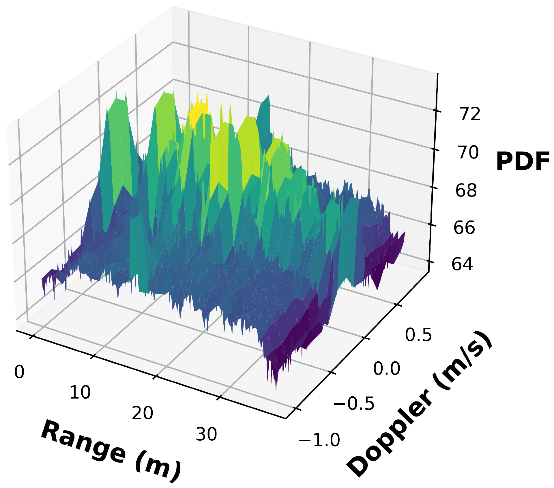
2.1.1. Wavelet Denoising

The initial stage in refining the quality of range-Doppler data, often plagued by various environmental noise sources [24], involves the application of a discrete wavelet transform (DWT) [25]. Initially, the original range-Doppler matrix ( R D ) is decomposed into approximation ( A L L ) and detail coefficients ( H L , V L , D L L ) through a 2D wavelet transform [26].
T ( x ) = s i g n ( x ) × m a x ( | x | λ )
The threshold function T ( x ) , where x is any given element on the range-Doppler matrix given in Equation (4), subtracts a threshold value λ from the absolute value of a specific element from the range-Doppler matrix. As a result, noise below a specific significance level (specified by the value of λ ) is effectively suppressed. The s i g n ( x ) function keeps the element’s sign, which is important since it keeps the directional information associated with the range-Doppler data.
Subsequently, the thresholding operation is applied individually to the horizontal ( H L ), vertical ( V L ), and diagonal ( D L L ) detail coefficients. The denoised range-Doppler matrix ( R D d e n o i s e d ) is then reconstructed by combining the approximation coefficients with the modified detail coefficients. The denoised range-Doppler data are shown in Figure 3.
The wavelet denoiser helps clean unwanted noise associated with the received range-Doppler data from the radar, shown in Figure 3.

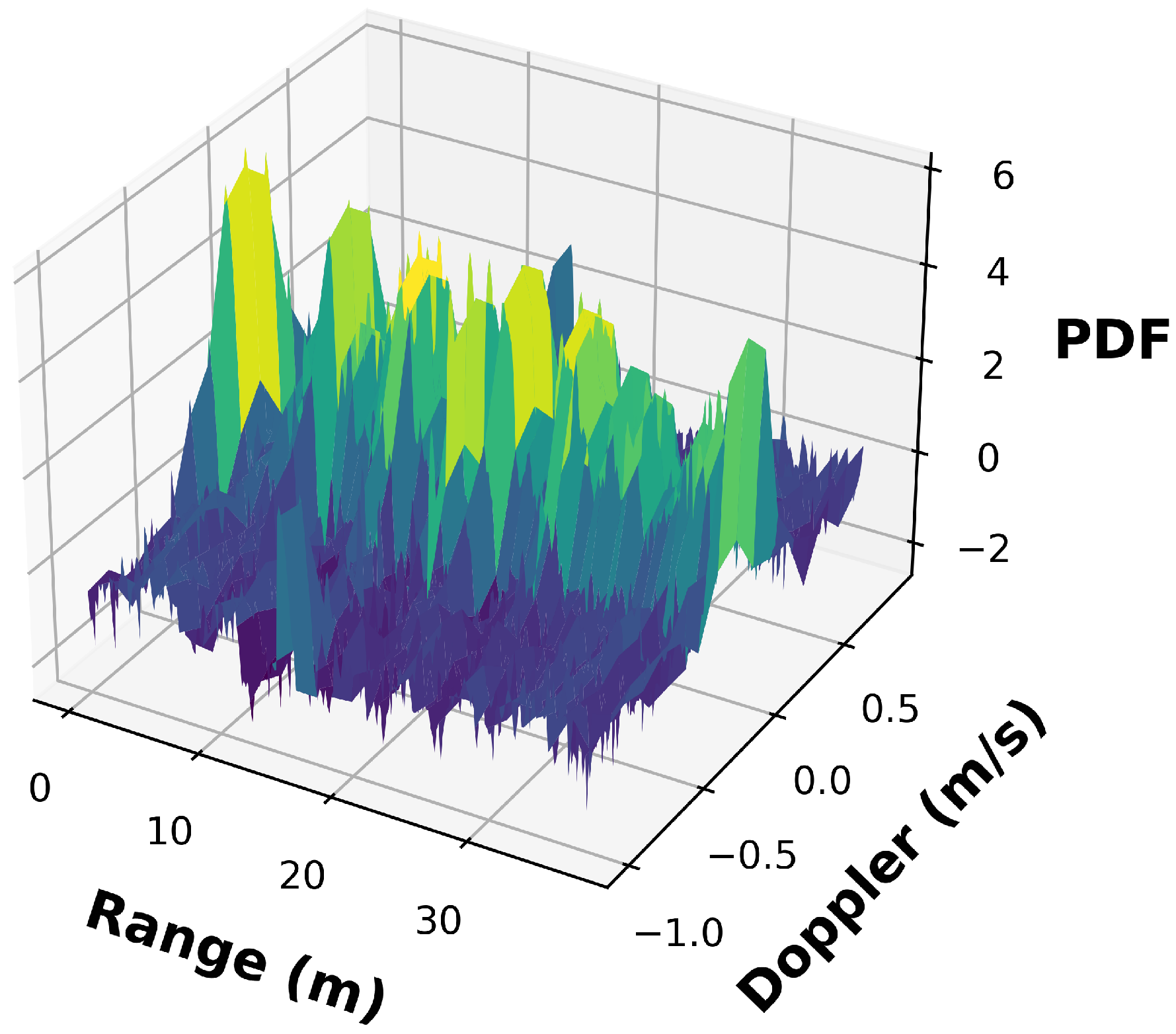
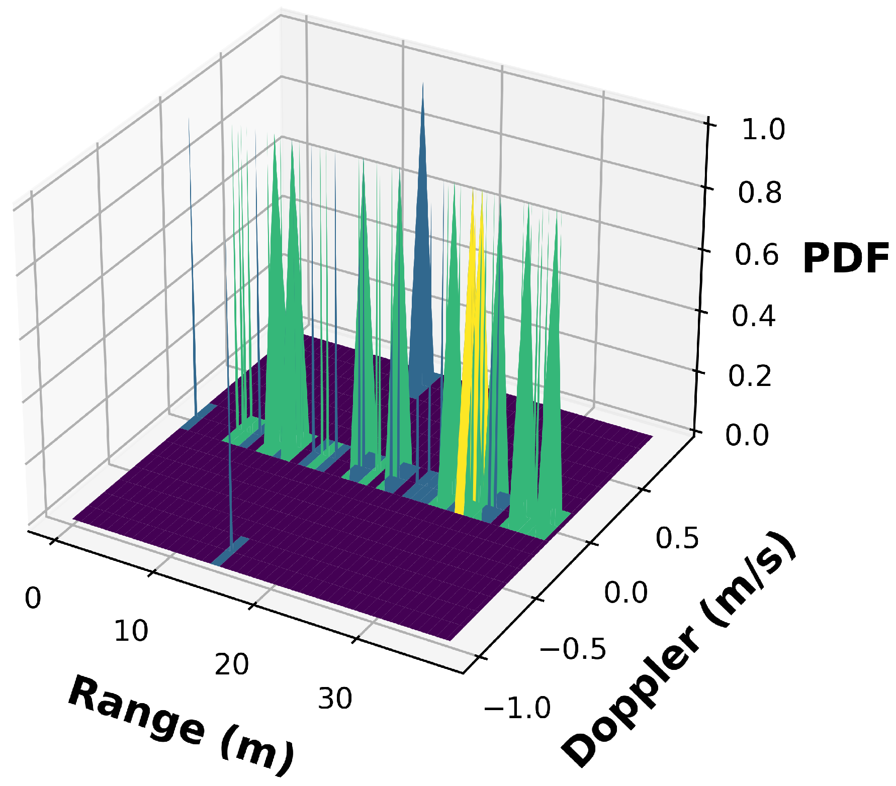
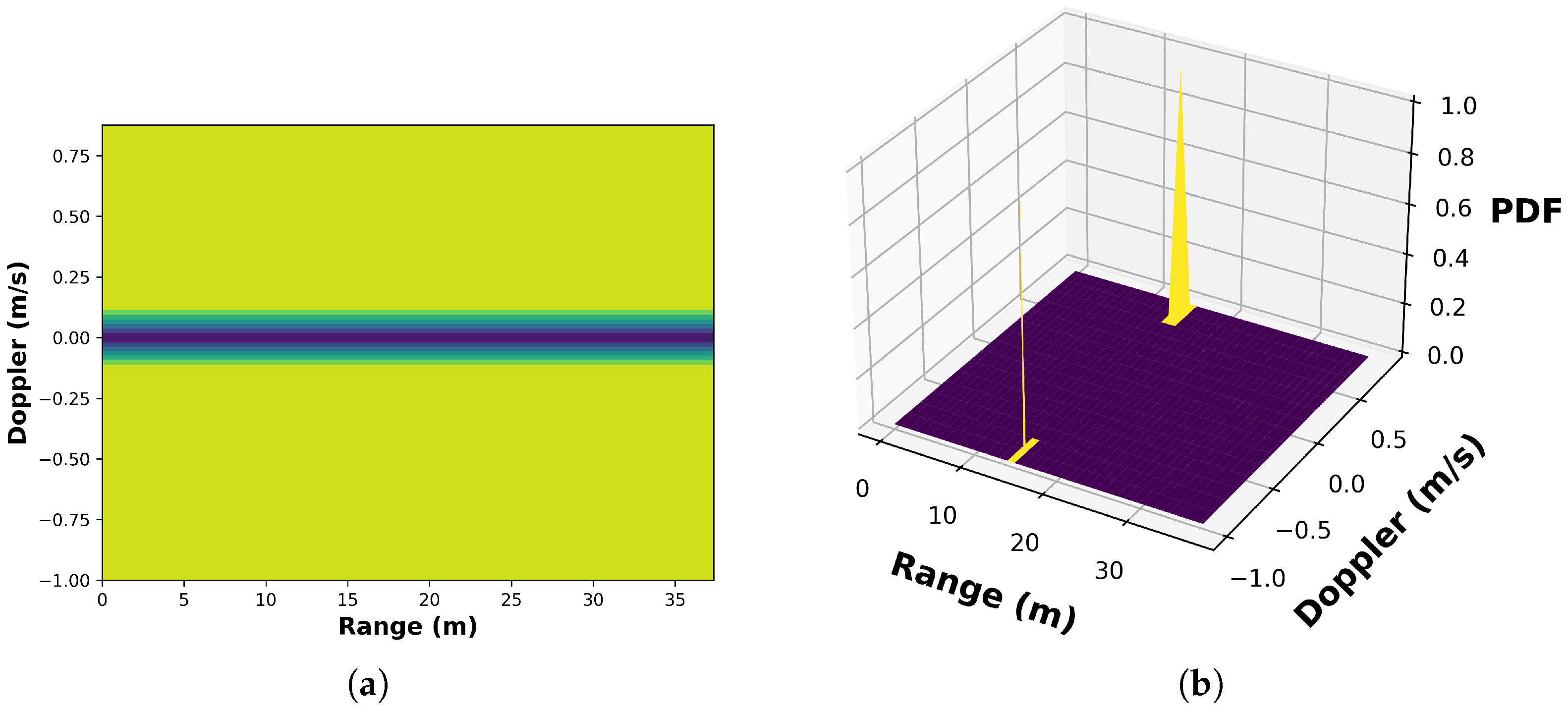
2.1.2. Doppler Filtering

The denoised data obtained from the previous processing stage are subsequently input into a Doppler filter [27]. This filter is used to bolster the radar system’s capacity to detect and distinguish moving targets, all while effectively suppressing stationary clutter and unwanted noise. The denoised radar data matrix ( R D d e n o i s e d ), undergoes a convolution operation with Doppler filter coefficients h. The filtered data Y is obtained by convolving each column of R D d e n o i s e d with the filter coefficients h. The convolution operation can be expressed mathematically as Equation (5), which captures the relationship between the input radar data and the Doppler filter [28].
R D f i l t e r e d [ n ] = k = 0 N 1 R D d e n o i s e d [ n k ] h [ k ]
where, R D f i l t e r e d [ n ] is the value at position n column of the filtered data, h [ k ] denotes the kth filter coefficients, and R D d e n o i s e d [ n k ] is the value at position n k of the radar data [29]. The filtered range-Doppler data are shown in Figure 4.

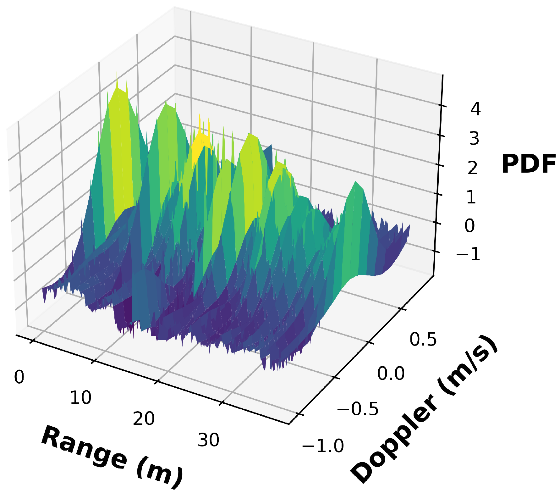
2.1.3. Peak Detection

The filtered range-Doppler data from the previous section contains the intensity of the reflected signals at different ranges and Doppler frequencies. Therefore, to identify targets that reflect radar signals the range-Doppler data from the radar are subjected to peak detection [30]. The range-Doppler matrix with elements R D f i l t e r e d [ i , j ] , where i represents the range index and j the Doppler frequency index is subjected to peak detection as given in Equation (6).
Peak [ i , j ] = 1 , i f R D f i l t e r e d [ i , j ] ( t o p , b o t t o m , l e f t , r i g h t ) and R D f i l t e r e d [ i , j ] threshold , 0 , otherwise .
where, t o p = R D f i l t e r e d [ i 1 , j ] is the element corresponding to the range above the current range, b o t t o m = R D f i l t e r e d [ i + 1 , j ] is the element corresponding to the range below the current range, l e f t = R D f i l t e r e d [ i , j 1 ] is the element corresponding to the Doppler frequency to the left of the current frequency and r i g h t = R D f i l t e r e d [ i , j + 1 ] is the element corresponding to the Doppler frequency to the right of the current frequency. However, to discern and eliminate the peaks associated with objects having zero Doppler frequency, notably visible as a central band in Figure 5, a targeted correction is applied. To achieve this, the range-Doppler data undergo a multiplication process with a two-dimensional mask (shown in Figure 6a).
This mask is strategically designed with zero values in its central cells, effectively creating a void in the area corresponding to stationary objects. Subsequently, this mask is multiplied with the matrix containing the detected peaks, selectively nullifying contributions from stationary objects in the central band while retaining those associated with moving targets. The outcome of this mask multiplication is reflected in Figure 6b, illustrating the processed peak detection output after applying the mask.
The range-Doppler matrix obtained after the previous steps contains peaks (with value 1) for an object with some Doppler frequency as seen in Figure 6b. When dealing with moving objects, these peaks shift cell by cell in the processed range-Doppler plot as it accumulates over time [31]. To determine whether the object is in motion or stationary, a temporal stacking operation is applied to the range-Doppler matrix. The resulting array undergoes threshold evaluation, with the threshold determined through experimentation. If any element in the stacked array surpasses this threshold, the system classifies the outcome as “Moving target detected”. Conversely, if all elements remain below the threshold, the classification is “No moving target detected”. This stacking and threshold-based classification are repeated for every five consecutive frames of the range-Doppler plot, providing a systematic way to identify the presence of moving targets.

3. Experiment, Results, and Discussion

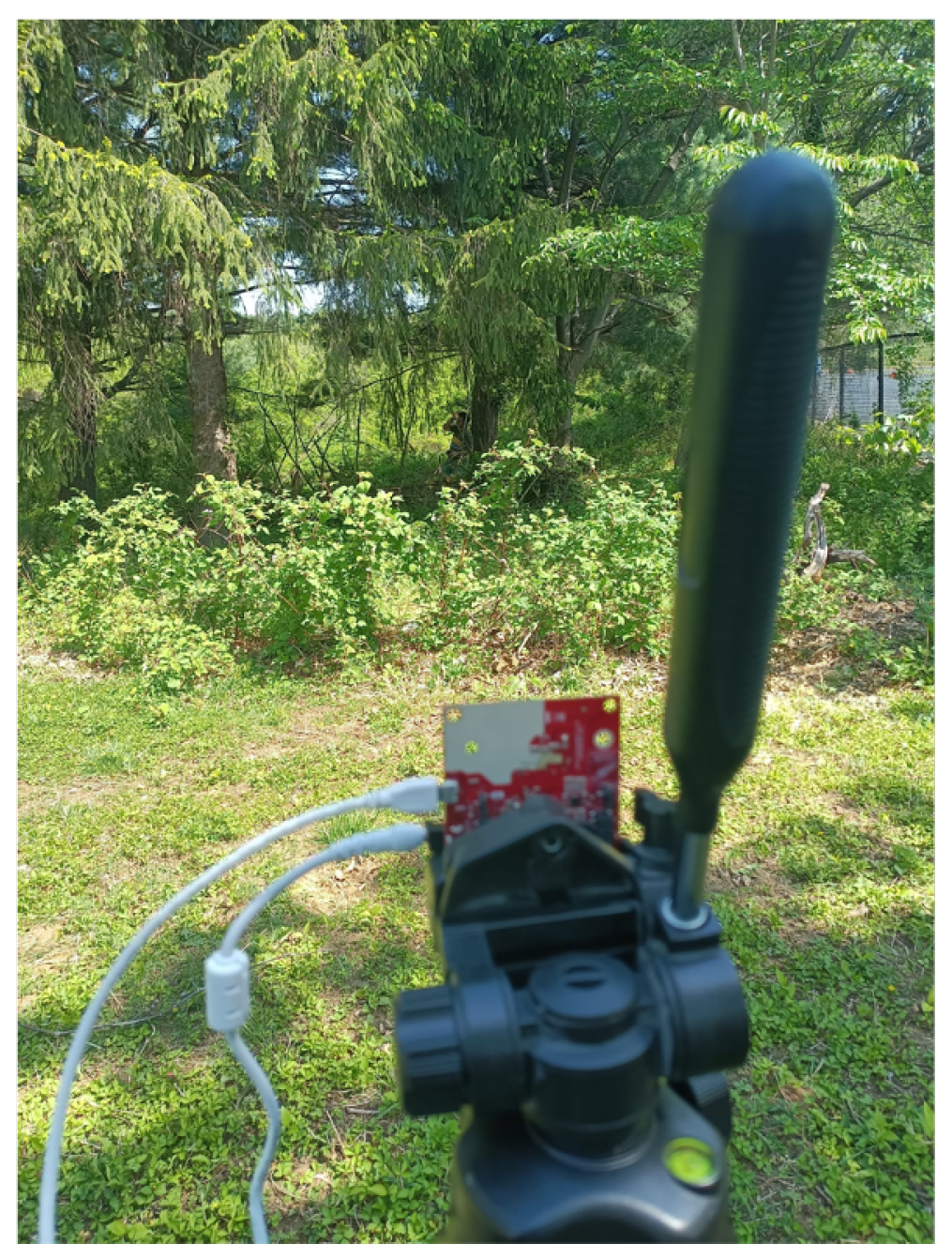
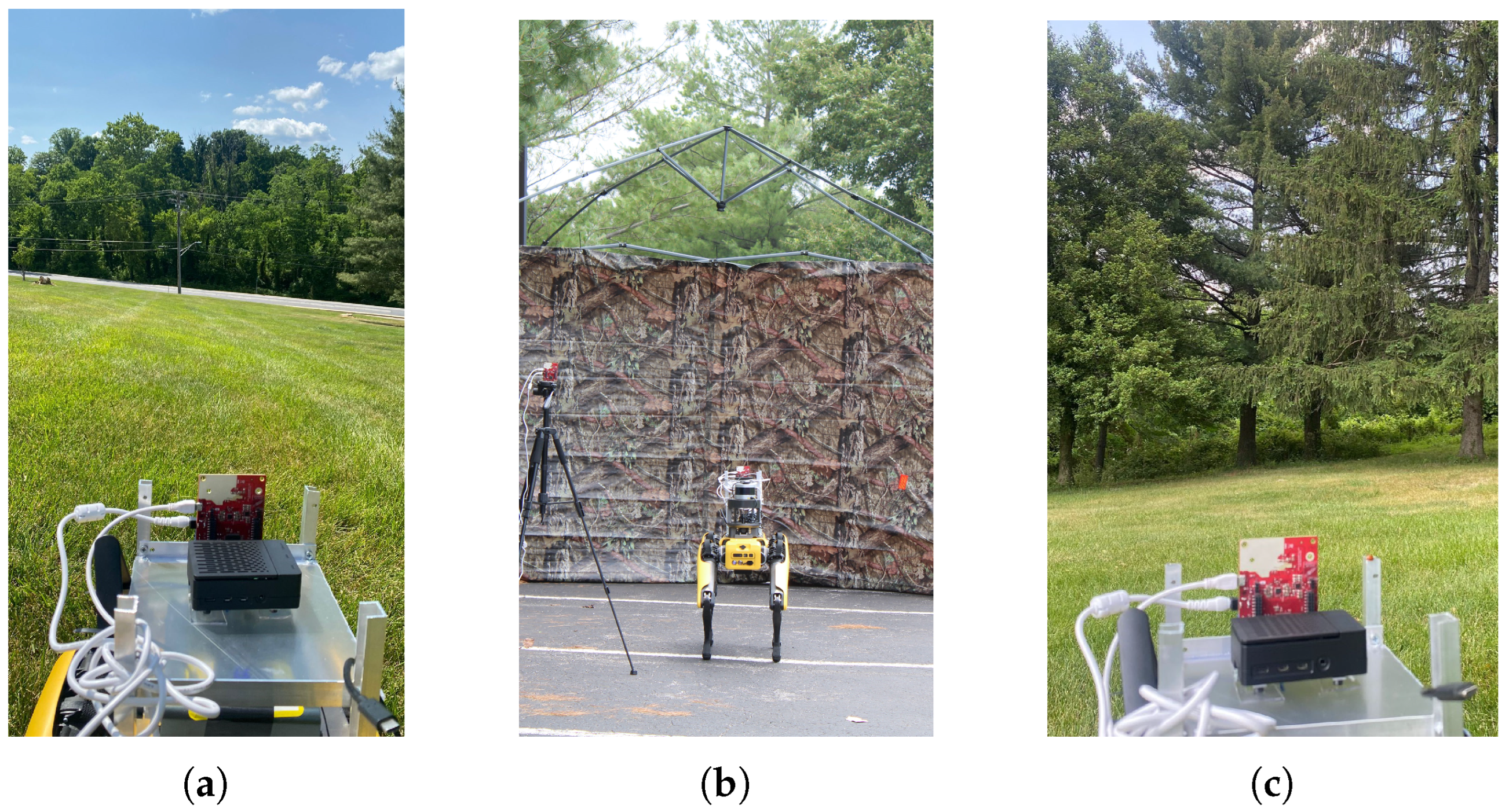
3.1. Experimental Setup

The experimental setup for evaluating the proposed moving target identification system was carefully designed to ensure accurate and reliable results. The setup was situated in an open area within the Center for Real-time Distributed Sensing and Autonomy at the University of Maryland, Baltimore County, as shown in Figure 7. This location provided a controlled environment free from external interference, allowing for precise data collection and analysis. The core components of the experimental setup included a Texas Instruments AWR1642 BOOST mmWave radar sensor and a Raspberry Pi single-board computer.
The mmWave radar sensor, equipped with two transmit antennas and four receiving antennas [32], was the primary sensing device responsible for detecting and tracking a moving person. In this setup, four receive antennas capture signals from varied angles, enhancing Doppler shift information. Simultaneously, two transmit antennas create multiple beams, offering coverage flexibility and enabling beam steering for improved radar performance. The Raspberry Pi served as the data acquisition and processing platform, capturing and processing the radar sensor’s output signals. The mmWave radar sensor’s configuration was optimized to achieve the desired performance characteristics. It transmitted 256 chirps using each coherent processing interval (CPI), with a bandwidth of 3 GHz and a duration of 51.2 s. This configuration resulted in a range resolution of 0.146 m, a velocity resolution of 1.0018 m per second (m/s), and a maximum range of 33.75 m. These parameters were carefully chosen to balance the trade-offs between range resolution, velocity resolution, and maximum range, ensuring that the system could effectively detect and track moving targets within the specified range and velocity range. The signal processing pipeline from the previous section is implemented in Python language [33], and the entire software stack is deployed on the Raspberry Pi acting as the data acquisition and processing platform. The Raspberry Pi’s capabilities were sufficient to handle the real-time data processing demands of the radar sensor, while its compact size and low power consumption made it a suitable choice for field testing and deployment.

3.2. Experimental Results

In this section, the accuracy results in terms of a binary classification problem are presented. In this case, the classes “Moving target detected” and “No moving target detected” are considered. The following notations are used when a total of 1000 tests were performed, 650 True positives (TP) are moving targets detected correctly classified, 60 false positives (FP) are non-moving targets incorrectly classified as moving, 270 true negatives (TN) are non-moving targets correctly classified, 20 false negatives (FN) are moving targets incorrectly classified as non-moving. The following metrics are then adopted:
  • Accuracy (Acc.), Acc = TP+TN/TP+TN+FP+FN, indicates the correctness of the classifications.
  • Precision (PR), PR = TP/TP+FP, indicates how many predicted positive labels are positive.
  • Sensitivity (SE), SE = TP/TP+FN, indicates how much a model is accurate to predict the positive class
  • Specificity (SP), SP= TN/TN+FP, indicates how much a model is accurate to predict the negative class.
The results are presented in Table 1 proves that the proposed system is capable of distinguishing moving targets from non-moving ones.

3.3. Comparison with Similar Techniques

The work described here in this paper is directly compared with various state-of-the-art approaches, as outlined in Table 2, by taking the developed MTD algorithm along with a couple of techniques available in the literature for field trial as seen in Figure 8.
The evaluation spanned diverse environmental scenarios, ranging from the first environment characterized by minimal foliage, through the second environment with a moderate density of foliage, to the final environment featuring the maximum density of foliage shown in Figure 8. Throughout these experiments, the targeted moving object maintained a consistent distance of 30 m from the mmWave Radar. It is worth emphasizing the noteworthy progress observed in the field of moving target detection, a fact corroborated by the impressive advancements documented in prior studies, specifically references [34,35]. In these seminal works, the authors demonstrated remarkable accuracy rates, achieving 98.7% and 99.75%, respectively. Notably, these exceptional outcomes were realized by employing cutting-edge deep learning-based classifier architectures, such as Convolutional Neural Networks (CNN) and SqueezeNet. A similar scenario can be seen in the case of [36,37,38,39,40], where the accuracy of the detection technique falls as the environment becomes cluttered. This comparison serves to underscore the significance of our newly proposed methodology, as it not only competes favorably with these highly advanced approaches but, importantly, showcases its own merits, particularly in scenarios characterized by varying levels of foliage density.
The rigorous evaluation process validates the robustness and adaptability of our moving target identification system, affirming its potential as a leading solution in the ever-evolving landscape of advanced radar-based sensing systems.

3.4. Comparison Based on Computational Complexity

The computational complexity of the developed radar signal processing pipeline is very critical for real-time applications. The wavelet filtering, applied to the range-Doppler data in the very first step, exhibits a typical complexity of O ( N ) [41], where N represents the size of the input signal (in this case, 16 by 256). Simultaneously, Doppler processing involves techniques such as the Fast Fourier Transform (FFT) in the Doppler domain, which comes with a complexity of O ( N d l o g N d ) , where N d is the number of Doppler bins. However, in the case of CNNs, the computational complexity of a convolutional layer is often expressed as O ( K N M ) , where K is the number of filters, N is the size of the input feature map, and M is the size of the filter. Similarly, for pooling operations, complexity is generally lower than convolution, often O ( P ) , where P is the number of pooling operations [42]. After convolutional and pooling layers, fully connected layers involve matrix multiplications. If F is the number of neurons in the fully connected layer, the complexity is O ( F C ) , where C is the number of input neurons.

4. Conclusions

In conclusion, this paper presents an innovative approach to moving target detection using the AWR 1642 BOOST mmWave Radar. Our digital signal processing pipeline, consisting of a wavelet denoiser, pulse Doppler filter, and peak detection algorithm, outperforms traditional machine learning-based methods. Our approach’s effectiveness is demonstrated by transforming peak data into a 5 × 2 matrix and applying a threshold test, yielding an impressive accuracy rate of 92.0% (seen in Table 1). It can be observed from Table 2 that the methodology proposed here in this work is not as accurate as MTD applications that use learning-based techniques at a much lower computational complexity, as discussed in Section 3.3. However, it can also be seen from Table 2 that the proposed techniques suffer less degradation when the type of environment changes. Hence, in applications requiring precise target detection, such as autonomous vehicles and surveillance systems [43], our method represents a significant advancement this technique will prove advantageous. In subsequent research, we will use radars that are capable of overcoming the speed and range resolution constraints to address the multi-target categorization challenge using a similar DSP-based technique.

Author Contributions

Conceptualization, D.C., B.P. and A.G.; Data curation, N.V.M. All authors have read and agreed to the published version of the manuscript.

Funding

This research is supported by U.S. Army Grant No. W911NF2120076.

Data Availability Statement

Data are contained within the article.

Conflicts of Interest

The authors declare no conflict of interest.

References

  1. Yadav, S.S.; Agarwal, R.; Bharath, K.; Rao, S.; Thakur, C.S. TinyRadar: MmWave radar based human activity classification for edge computing. In Proceedings of the 2022 IEEE International Symposium on Circuits and Systems (ISCAS), Austin, TX, USA, 27 May–1 June 2022; pp. 2414–2417. [Google Scholar]
  2. Lee, M.J.; Kim, J.E.; Ryu, B.H.; Kim, K.T. Robust Maritime Target Detector in Short Dwell Time. Remote Sens. 2021, 13, 1319. [Google Scholar] [CrossRef]
  3. Petrovskaya, A.; Thrun, S. Model based vehicle detection and tracking for autonomous urban driving. Auton. Robot. 2009, 26, 123–139. [Google Scholar] [CrossRef]
  4. Goswami, P.; Rao, S.; Bharadwaj, S.; Nguyen, A. Real-time multi-gesture recognition using 77 GHz FMCW MIMO single chip radar. In Proceedings of the 2019 IEEE International Conference on Consumer Electronics (ICCE), Las Vegas, NV, USA, 11–13 January 2019; pp. 1–4. [Google Scholar]
  5. Yan, H.; Chen, C.; Jin, G.; Zhang, J.; Wang, X.; Zhu, D. Implementation of a modified faster R-CNN for target detection technology of coastal defense radar. Remote Sens. 2021, 13, 1703. [Google Scholar] [CrossRef]
  6. Lin, Z.; Niu, H.; An, K.; Hu, Y.; Li, D.; Wang, J.; Al-Dhahir, N. Pain without Gain: Destructive Beamforming from A Malicious RIS Perspective in IoT Networks. IEEE Internet Things J. 2023; early access. [Google Scholar] [CrossRef]
  7. Lin, Z.; Lin, M.; Champagne, B.; Zhu, W.P.; Al-Dhahir, N. Secrecy-energy efficient hybrid beamforming for satellite-terrestrial integrated networks. IEEE Trans. Commun. 2021, 69, 6345–6360. [Google Scholar] [CrossRef]
  8. An, K.; Lin, M.; Ouyang, J.; Zhu, W.P. Secure transmission in cognitive satellite terrestrial networks. IEEE J. Sel. Areas Commun. 2016, 34, 3025–3037. [Google Scholar] [CrossRef]
  9. Lin, Z.; Niu, H.; An, K.; Wang, Y.; Zheng, G.; Chatzinotas, S.; Hu, Y. Refracting RIS-aided hybrid satellite-terrestrial relay networks: Joint beamforming design and optimization. IEEE Trans. Aerosp. Electron. Syst. 2022, 58, 3717–3724. [Google Scholar] [CrossRef]
  10. Jin, F.; Zhang, R.; Sengupta, A.; Cao, S.; Hariri, S.; Agarwal, N.K.; Agarwal, S.K. Multiple patients behavior detection in real-time using mmWave radar and deep CNNs. In Proceedings of the 2019 IEEE Radar Conference (RadarConf), Boston, MA, USA, 22–26 April 2019; pp. 1–6. [Google Scholar]
  11. Jiang, W.; Ren, Y.; Liu, Y.; Leng, J. Artificial neural networks and deep learning techniques applied to radar target detection: A review. Electronics 2022, 11, 156. [Google Scholar] [CrossRef]
  12. Liang, S.; Chen, R.; Duan, G.; Du, J. Deep learning-based lightweight radar target detection method. J. Real-Time Image Process. 2023, 20, 61. [Google Scholar] [CrossRef]
  13. Kavitha, V.; Prabakar, D.; subramanian, S.R.; Balambigai, S. Radar optical communication for analysing aerial targets with frequency bandwidth and clutter suppression by boundary element mmwave signal model. Opt. Quantum Electron. 2023, 55, 1142. [Google Scholar] [CrossRef]
  14. Renhe, L.; Renli, Z.; Tiancheng, L.; Weixing, S. ISRJ identification method based on Chi-square test and range equidistant detection. In Proceedings of the 2023 International Conference on Microwave and Millimeter Wave Technology (ICMMT), Qingdao, China, 14–17 May 2023; pp. 1–3. [Google Scholar]
  15. Kuang, C.; Wang, C.; Wen, B.; Hou, Y.; Lai, Y. An improved CA-CFAR method for ship target detection in strong clutter using UHF radar. IEEE Signal Process. Lett. 2020, 27, 1445–1449. [Google Scholar] [CrossRef]
  16. Li, Y.; Zhang, G.; Doviak, R.J. Ground clutter detection using the statistical properties of signals received with a polarimetric radar. IEEE Trans. Signal Process. 2013, 62, 597–606. [Google Scholar] [CrossRef]
  17. Chen, X.; Guan, J.; Bao, Z.; He, Y. Detection and extraction of target with micromotion in spiky sea clutter via short-time fractional Fourier transform. IEEE Trans. Geosci. Remote Sens. 2013, 52, 1002–1018. [Google Scholar] [CrossRef]
  18. Anghel, A.; Vasile, G.; Cacoveanu, R.; Ioana, C.; Ciochina, S. Short-range wideband FMCW radar for millimetric displacement measurements. IEEE Trans. Geosci. Remote Sens. 2014, 52, 5633–5642. [Google Scholar] [CrossRef]
  19. Iyer, N.C.; Pillai, P.; Bhagyashree, K.; Mane, V.; Shet, R.M.; Nissimagoudar, P.; Krishna, G.; Nakul, V. Millimeter-wave AWR1642 RADAR for obstacle detection: Autonomous vehicles. In Proceedings of the Innovations in Electronics and Communication Engineering: Proceedings of the 8th ICIECE 2019, Hyderabad, India, 2–3 August 2019; Springer: Berlin/Heidelberg, Germany, 2020; pp. 87–94. [Google Scholar]
  20. Jeng, S.L.; Chieng, W.H.; Lu, H.P. Estimating speed using a side-looking single-radar vehicle detector. IEEE Trans. Intell. Transp. Syst. 2013, 15, 607–614. [Google Scholar] [CrossRef]
  21. Jankiraman, M. FMCW Radar Design; Artech House: Norwood, MA, USA, 2018. [Google Scholar]
  22. Richards, M.A. Fundamentals of Radar Signal Processing; Mcgraw-Hill: New York, NY, USA, 2005; Volume 1. [Google Scholar]
  23. Tavanti, E.; Rizik, A.; Fedeli, A.; Caviglia, D.D.; Randazzo, A. A short-range FMCW radar-based approach for multi-target human-vehicle detection. IEEE Trans. Geosci. Remote Sens. 2021, 60, 2003816. [Google Scholar] [CrossRef]
  24. Su, B.Y.; Ho, K.; Rantz, M.J.; Skubic, M. Doppler radar fall activity detection using the wavelet transform. IEEE Trans. Biomed. Eng. 2014, 62, 865–875. [Google Scholar] [CrossRef]
  25. Lee, S.; Lee, J.Y.; Kim, S.C. Mutual interference suppression using wavelet denoising in automotive FMCW radar systems. IEEE Trans. Intell. Transp. Syst. 2019, 22, 887–897. [Google Scholar] [CrossRef]
  26. Jin, Y.; Duan, Y. 2d wavelet decomposition and fk migration for identifying fractured rock areas using ground penetrating radar. Remote Sens. 2021, 13, 2280. [Google Scholar] [CrossRef]
  27. Fitasov, E.; Legovtsova, E.; Pal’guev, D.; Kozlov, S.; Saberov, A.; Borzov, A.; Vasil’ev, D. Experimental estimation of the projection method of the doppler filtering of radar signals when detecting air objects with low radial velocities. Radiophys. Quantum Electron. 2022, 64, 300–308. [Google Scholar] [CrossRef]
  28. Xu, J.; Yu, J.; Peng, Y.N.; Xia, X.G. Radon-Fourier transform for radar target detection, I: Generalized Doppler filter bank. IEEE Trans. Aerosp. Electron. Syst. 2011, 47, 1186–1202. [Google Scholar] [CrossRef]
  29. Papić, V.D.; Đurović, Ž.M.; Kvaščev, G.S.; Tadić, P.R. A new approach to Doppler filter adaptation in radar systems. In Proceedings of the 2011 19thTelecommunications Forum (TELFOR) Proceedings of Papers, Belgrade, Serbia, 22–24 November 2011; pp. 707–714. [Google Scholar]
  30. Kim, J.Y.; Park, J.H.; Jang, S.Y.; Yang, J.R. Peak detection algorithm for vital sign detection using Doppler radar sensors. Sensors 2019, 19, 1575. [Google Scholar] [CrossRef] [PubMed]
  31. Tabassum, N.; Vaccari, A.; Acton, S. Speckle removal and change preservation by distance-driven anisotropic diffusion of synthetic aperture radar temporal stacks. Digit. Signal Process. 2018, 74, 43–55. [Google Scholar] [CrossRef]
  32. Pirkani, A.; Pooni, S.; Cherniakov, M. Implementation of mimo beamforming on an ots fmcw automotive radar. In Proceedings of the 2019 20th International Radar Symposium (IRS), Ulm, Germany, 26–28 June 2019; pp. 1–8. [Google Scholar]
  33. Python Releases for Windows. Available online: https://www.python.org/downloads/windows/ (accessed on 24 June 2021).
  34. Dai, Y.; Liu, D.; Hu, Q.; Yu, X. Radar Target Detection Algorithm Using Convolutional Neural Network to Process Graphically Expressed Range Time Series Signals. Sensors 2022, 22, 6868. [Google Scholar] [CrossRef] [PubMed]
  35. Li, G.; Tong, N.; Zhang, Y.; Feng, W.; Liu, C. Moving Target Detection Classifier for Airborne Radar Using SqueezeNet. J. Phys. Conf. Ser. 2021, 1883, 012003. [Google Scholar] [CrossRef]
  36. Tang, X.; Chen, W.; Zhu, W. Radar emitter recognition method based on AdaBoost and decision tree. In Proceedings of the 2017 2nd International Conference on Automation, Mechanical Control and Computational Engineering (AMCCE 2017), Beijing, China, 25–26 March 2017; pp. 326–330. [Google Scholar]
  37. Patel, K.; Rambach, K.; Visentin, T.; Rusev, D.; Pfeiffer, M.; Yang, B. Deep learning-based object classification on automotive radar spectra. In Proceedings of the 2019 IEEE Radar Conference (RadarConf), Boston, MA, USA, 22–26 April 2019; pp. 1–6. [Google Scholar]
  38. Xie, R.; Sun, Z.; Wang, H.; Li, P.; Rui, Y.; Wang, L.; Bian, C. Low-resolution ground surveillance radar target classification based on 1D-CNN. In Proceedings of the Eleventh International Conference on Signal Processing Systems, Chengdu, China, 15–17 November 2019; Volume 11384, pp. 199–204. [Google Scholar]
  39. Xie, R.; Dong, B.; Li, P.; Rui, Y.; Wang, X.; Wei, J. Automatic target recognition method for low-resolution ground surveillance radar based on 1D-CNN. In Proceedings of the Twelfth International Conference on Signal Processing Systems, Shanghai, China, 6–9 November 2021; Volume 11719, pp. 48–55. [Google Scholar]
  40. Jiang, W.; Ren, Y.; Liu, Y.; Leng, J. A method of radar target detection based on convolutional neural network. Neural Comput. Appl. 2021, 33, 9835–9847. [Google Scholar] [CrossRef]
  41. Wen, M.; Zheng, B.; Kim, K.J.; Di Renzo, M.; Tsiftsis, T.A.; Chen, K.C.; Al-Dhahir, N. A survey on spatial modulation in emerging wireless systems: Research progresses and applications. IEEE J. Sel. Areas Commun. 2019, 37, 1949–1972. [Google Scholar] [CrossRef]
  42. Li, J.; Dang, S.; Wen, M.; Li, Q.; Chen, Y.; Huang, Y.; Shang, W. Index modulation multiple access for 6G communications: Principles, applications, and challenges. IEEE Netw. 2023, 37, 52–60. [Google Scholar] [CrossRef]
  43. Turpin, J.P.; Sieber, P.E.; Werner, D.H. Absorbing ground planes for reducing planar antenna radar cross-section based on frequency selective surfaces. IEEE Antennas Wirel. Propag. Lett. 2013, 12, 1456–1459. [Google Scholar] [CrossRef]
Figure 1. The raw range-Doppler data obtained from the Radar.
Electronics 12 05030 g001
Figure 2. The signal processing pipeline for the Radar.
Electronics 12 05030 g002
Figure 3. Wavelet denoised range-Doppler data from the Radar.
Electronics 12 05030 g003
Figure 4. Processed range-Doppler data after Doppler filter.
Electronics 12 05030 g004
Figure 5. The processed range-Doppler data.
Electronics 12 05030 g005
Figure 6. The peak detection algorithm (a) with zero Doppler frequency elimination mask and (b) masked to remove chirp returns from objects with zero Doppler frequency (stationary).
Electronics 12 05030 g006
Figure 7. The experiment setup with AWR1642 BOOST mmWave radar, mounted on tripod.
Electronics 12 05030 g007
Figure 8. The experimental setup with AWR1642 BOOST mmWave radar at (a) an empty landscape (b) a moderately dense and (c) a dense foliage environment.
Electronics 12 05030 g008
Table 1. Experimental results from a controlled lab environment.
S No.MetricsValues
1Accuracy (Acc.)0.920
2Precision (PR)0.915
3Sensitivity (SE)0.970
4Specificity (SP)0.818
Table 2. Comparison with similar moving target detection techniques.
S No.FrameworkDetectionPeak Accuracy
FeaturesArchitectureFirst
Environment
Second
Environment
Third
Environment
1This workRange-DopplerDoppler filter
with thresholding
91.2%90.8%91.3%
2Yan Dai, et al. [34]Range-DopplerCNN98.7%90.6%87.6%
3Li, et al. [35]Range-DopplerSqueezeNet99.75%96.12%95.23%
4Tang, et al. [36]Range-DopplerAdaBoost93.78%90.11%89.23%
5Patel, et al. [37]Range-DopplerCNN98.11%91.20%88.23%
6Xie, et al. [38]Range-Doppler1D-CNN98.0%97.2%96.3%
7Xie, et al. [39]Range-Doppler1D-CNN99.0%98.1%97.8%
8Jiang, et al. [40]Raw dataCNN98.5%97.7%96.4%
Disclaimer/Publisher’s Note: The statements, opinions and data contained in all publications are solely those of the individual author(s) and contributor(s) and not of MDPI and/or the editor(s). MDPI and/or the editor(s) disclaim responsibility for any injury to people or property resulting from any ideas, methods, instructions or products referred to in the content.

