Vehicle Simulation Algorithm for Observations with Variable Dimensions Based on Deep Reinforcement Learning

Abstract

Vehicle simulation algorithms play a crucial role in enhancing traffic efficiency and safety by predicting and evaluating vehicle behavior in various traffic scenarios. Recently, vehicle simulation algorithms based on reinforcement learning have demonstrated excellent performance in practical tasks due to their ability to exhibit superior performance with zero-shot learning. However, these algorithms face challenges in field adaptation problems when deployed in task sets with variable-dimensional observations, primarily due to the inherent limitations of neural network models. In this paper, we propose a neural network structure accommodating variations in specific dimensions to enhance existing reinforcement learning methods. Building upon this, a scene-compatible vehicle simulation algorithm is designed. We conducted experiments on multiple tasks and scenarios using the Highway-Env traffic environment simulator. The results of our experiments demonstrate that the algorithm can successfully operate on all tasks using a neural network model with fixed shape, even with variable-dimensional observations. Our model exhibits no degradation in simulation performance when compared to the baseline algorithm.

1. Introduction

The primary objective of vehicle simulation is to emulate potential vehicle trajectories within the traffic system, enabling prediction of vehicle behavior in various traffic scenarios. Vehicle simulation provides substantial simulated data support for various downstream tasks across diverse scenarios. Consequently, it plays a crucial role in practical applications. Dawood et al. [1] utilized a knowledge-driven simulation system to seek reliable road construction strategies, thereby preventing wasted resources. Gambardella et al. [2] incorporated the simulation system into the combined rail/road transport system, which improved the operational efficiency of the system. Wang et al. [3] deployed vehicle simulation methods in the context of path planning and devised individualized driving trajectories for vehicles by setting constraint factors. Aycin et al. [4] investigated car-following models using simulation algorithms, with Li et al. [5] providing a thorough analysis and proposing vehicular congestion control strategies based on these models. Building upon this, Wang et al. [6] used vehicle simulation techniques to investigate intersection traffic scenarios and formulated car-following and lane-changing rules applicable to varied traffic conditions. Krajzewicz et al. [7] followed similar methods and proposed an efficient traffic signal light control method. Considering that these tasks are oriented towards real-world scenarios, the design of a simulation algorithm capable of adequately representing real-world characteristics has long been a focal point in academic research.

Traditional vehicle simulation algorithms typically employ mathematical models to describe the driving of vehicles within traffic systems [8,9]. These mathematical models often focus on the primary factors influencing vehicles, such as lead vehicle speed and inter-vehicle gaps [10], and possess strong interpretability [11]. However, due to the constraints of model complexity, these mathematical models are often only applicable to relatively simple traffic systems, such as the single-lane car-following model and simple intersections with few vehicles and influencing factors [12]. Describing complex traffic systems using mathematical models is exceedingly challenging due to the multitude of factors involved and the potential interactions among them, resulting in model distortion or rendering the construction of such mathematical models infeasible.

In recent years, with the rapid advancement of machine learning theories, an increasing number of researchers have begun to explore the use of deep neural networks to address complex scenarios that are difficult to simulate using traditional mathematical models [13], achieving remarkable results. Machine learning leverages neural networks with a large number of parameters to learn and analyze real-world data. For instance, machine learning has been utilized for the analysis of sandstorm conditions [14]. In the field of transportation, neural networks have been extensively deployed for the analysis of driver behavior [15] and for prediction of road traffic conditions [16], capturing intricate relationships among various influential factors. Consequently, it enables more accurate modeling of vehicle behavior and traffic conditions [17], thereby making vehicle simulations in complex environments possible. Regrettably, machine learning is a data-driven modeling approach, necessitating a large amount of data for model-learning to effectively extract implicit data features and patterns [18,19]. The demand for training data restricts the efficacy of such simulation methods in real-world scenarios that lack adequate data due to limited vehicular traffic or other related factors.

To solve the aforementioned shortcomings, some researchers have begun exploring self-supervised machine learning methods to alleviate the reliance on data [20]. Out of all the self-supervised learning algorithms, reinforcement learning methods are the most widespread and have been used to analyze car-following models [21], traffic signal control [22], and traffic scheduling problems [23]. In contrast to supervised learning, which relies on labeled data as input, reinforcement learning is a goal-driven method [24,25]. Researchers predefine the objectives they wish to achieve in specific environments and assign rewards based on the significance of attaining these objectives. The entity interacting with the environment, often referred to as the agent, learns through trial and error within the environment, reinforcing the strategy that led to a satisfactory reward. Vehicle simulation algorithms based on reinforcement learning have shown unexpected success, particularly in micro-level scenarios [26].

Considered from the perspective of current technological developments, the popularity of electric vehicles, represented by Tesla, has been booming in automotive markets worldwide [27], including Europe, the United States, and China. Consequently, the vehicle-control problem associated with autonomous vehicles is garnering increased attention from researchers [28]. Reinforcement learning methods, with their robust capability of interactions with the real-world, support making decisions in complex and uncertain environments, demonstrating adaptiveness and predictiveness. This has led to a majority of vehicle control techniques being grounded in reinforcement learning methods [29,30]. However, constrained by the mathematical nature of neural networks, reinforcement learning models require the observation dimensions provided by the environment to be fixed, otherwise rendering them inoperable within matrices of neural networks. In the real world, observation dimensions may fluctuate for various reasons. For instance, rainy or foggy conditions narrow visibility, while congested traffic increases the number of vehicles within the field of view. These variations pose challenges for reinforcement learning models. This challenge permeates not only vehicle-control problems but also the field of vehicle simulation, which suffers from the relationships between vehicles, thereby exacerbating the complexity of the issue [31].

In this paper, we construct a deep reinforcement learning neural network model capable of handling observations with variable dimensions. Building upon this, we propose a vehicle simulation algorithm that can be utilized across a set of traffic systems or scenarios where dimensions of observations may vary. The main contribution of this method lies in the design of processing networks that map variable-dimensional observations into fixed-dimensional feature matrices, integrating them into a deep neural network framework for reinforcement learning. This approach inherits advantages from both machine learning theory and reinforcement learning methods, enabling the algorithm to handle complex traffic systems, extract their inherent features, and, even in cases of limited or absent data, seek vehicle operational patterns and conduct vehicle simulations through goal-driven and trial-and-error approaches. These advantages can be extended within our framework to a broader range of traffic systems, particularly those involving tasks and scenarios with non-fixed observation dimensions. We illustrate the scalability of this structure, indicating that more advanced feature extraction and decision-making methods can be integrated into the neural network model.

To provide a more practical demonstration of the model’s applicability, we implemented our algorithm in the Highway-Env traffic environment simulator and conducted experiments on a diverse set of tasks with variable-dimensional observations. The results indicate that a neural network model with fixed shape can operate effectively across various scenarios, aligning the vehicle’s behavior with predetermined objectives, even when observation dimensions across tasks are dissimilar. A reasonable concern regarding this model pertains to the potential training difficulties posed by additional neural networks, thereby impacting the effectiveness of simulation results. We compared the results of our model with those of a baseline model, demonstrating that this structure does not compromise performance.

2. Related Work

2.1. Vehicle Simulation

The methods of vehicle simulation vary based on the granularity of the model tailored to practical demands. Generally, micro-level models focus on detailed representation of individual vehicles, considering interactions among vehicles and their interaction with the road network [32]. Conversely, macro-level traffic models employ aggregated variables and mathematical equations to describe traffic, emphasizing the overall properties of the traffic system, including macroscopic indicators such as speed, traffic flow, and traffic density. These models utilize large-scale data and variables to describe and predict traffic without involving the behavior of individual vehicles [33]. Given the focus of this paper on inter-vehicle interactions and vehicle behavior prediction, micro-level models are more relevant.

In the micro-level model, the primary mathematical approach is based on vehicle-following models. These models simulate highway traffic conditions through differential equations.The mathematical expression based on density is as follows:

$$\frac{d\rho }{dt}+\frac{d\left(Q\left(\rho \right)\right)}{dx}$$

(1)

In the above equation, the symbol $\rho$ represents traffic density (i.e., the number of vehicles per unit length), t represents time, and x denotes spatial coordinates. $Q\left(\rho \right)$ represents the flow-density relationship function, expressing the pattern of traffic flow variation with density. The specific form of the function $Q\left(\rho \right)$ depends on the traffic flow model employed. Taking the LWR model (Lighthill–Whitham–Richards model) as an example, its flow-density relationship typically manifests in the following form:

$$Q\left(\rho \right)=V\left(\rho \right)\times \rho$$

(2)

The model exhibits significant interpretability advantages and effectively describes real-world scenarios; however, it also possesses certain limitations, such as inadequate adaptation to characteristics of specific road segments or complex intersections.

Building upon this, some scholars have proposed behavior-based modeling approaches. Such approaches emphasize simulating the behavior and interactions of traffic participants to more accurately analyze real traffic phenomena. Taking cellular automata as an example, this approach discretizes intersections into a grid of cells to model vehicle movement. While this approach offers greater flexibility, its discretization may limit the model’s computational speed and accuracy [34]. Furthermore, heuristic-based driver task modeling approaches attempt to create agents capable of driving on the road, but they may struggle to fully simulate real driver behaviors [35].

2.2. Reinforcement Learning

Reinforcement learning is a subfield of machine learning and is typically characterized by an agent–environment framework [36]. In this framework, the agent selects actions to interact with the environment, altering the environmental state and obtaining pre-defined rewards [37]. Such interactions will be repeated over a sequence of timesteps until the environment emits the termination signal or the time limit is reached. Generally speaking, the interaction between agents and environment is modeled as a Markov decision process (MDP) [38], denoted as the tuple <$\mathcal{S},\mathcal{A},\mathcal{D},\mathcal{T},\mathcal{R}$>. $\mathcal{S}$ denotes the state space of the environment, while $\mathcal{A}$ represents the action space that the agent can choose from. $\mathcal{D}\in P\left(\mathcal{S}\right)$ signifies the probability distribution of the initial state within the state space, and $\mathcal{T}:\mathcal{S}\times \mathcal{A}\to P\left(\mathcal{S}\right)$ stands for the state transition probability function. $\mathcal{R}\in \mathcal{S}\times \mathcal{A}\times \mathcal{S}\to \mathbb{R}$ is the function that determines the rewards obtained by the agent. In the above definition, $P\left(\mathcal{S}\right)$ refers to a probability distribution over the state space $\mathcal{S}$.

The agent possesses a policy function $\pi \left(s\right):\mathcal{S}\to P\left(\mathcal{A}\right)$ for the selection action and interacts with the environment [39]. The policy function computes the probability distribution of selecting action a from the action space $\mathcal{S}$ when the agent is in a given state $s\in \mathcal{S}$. The aim of the agent is to accumulate as much total reward $R_{tot}={\sum }_{t=0}^{\infty }{R}_t$ as possible through its interactions with the environment. Considering the temporal effects, immediate rewards are preferred over delayed rewards of equal value. Therefore, an additional discount factor $\gamma \in \left[0,1\right]$ is introduced to decrease the value of future rewards, thus evaluating using the cumulative discounted reward $R_{tot}={\sum }_{t=0}^{\infty }{\gamma }^t{R}_t$. In order to optimize the policy of the agent, a series of tuples <$s_t,a_t,r_t,s_{t+1}$> is used to record the trajectory of the agent–environment interactions. $s_t$ is the state of the environment at time t. $a_t$ is the action taken by agent at time t. $r_t$ is the reward obtained by the agent at time t, and $s_{t+1}$ represents the state of the environment at time $t+1$. The agent needs to discern patterns of environmental changes and learn a policy that can maximize the rewards obtained.

The state value function $V^{\pi }\left(s\right)$ is defined as the expectation of a cumulative discounted reward obtained by the agent from state s to the end following policy $\pi$, denoted as $V^{\pi }\left(s\right)$:= $\mathbb{E}\left[{\sum }_{t=0}^{\infty }{\gamma }^t\mathcal{R}\left(s_t,a_t,s_{t+1}\right)|s_0=s;a_t\sim \pi \left(·|s_t\right)\right]$ [40]. Based on this, the state-action value function $Q^{\pi }\left(s,a\right)$:= $\mathbb{E}\left[{\sum }_{t=0}^{\infty }{\gamma }^t\mathcal{R}\left(s_t,a_t,s_{t+1}\right)|s_0=s;a_0=a;a_t\sim \pi \left(·|s_t\right)\right]$ is defined as the expectation of a cumulative discounted reward when selecting action a in state s. Considering its mathematical significance, a reasonable strategy is to greedily select the action that maximizes the reward expectations at each timestep, i.e., $\pi \left(s\right)$:= $\underset{a\in \mathcal{A}}{argmax}Q\left(s,a\right)$. This shifts the objective of reinforcement learning towards accurately estimating $V^{\pi }\left(s\right)$ and $Q^{\pi }\left(s,a\right)$ as much as possible.

2.3. Deep Q-Learning

The Bellman equation [41] establishes the relationship between the current state-action and the future state-action based on dynamic programming, i.e., $Q^{\pi }\left(s,a\right)$:= $\mathbb{E}[r_t+\gamma max$$Q^{\pi }\left(s_{t+1},a_{t+1}\right)|s_t=s;a_t=a]$. Building upon this, traditional Q-learning methods use a Q-table to estimate $V^{\pi }\left(s\right)$ and $Q^{\pi }\left(s,a\right)$ [42,43]. However, such methods suffer from the “curse of dimensionality” and cannot be applied to environments with a vast number of states. On one hand, the immense number of states would elevate the dimensionality of the table to unacceptable levels that cannot be recorded or calculated. On the other hand, exploration would make it difficult to traverse all possible states in the environment, with unexplored states posing a potentially destructive impact on the algorithm. Therefore, a computational model capable of handling a large number of states and robust to unvisited states is imperative.

With the development of deep neural networks, researchers have begun to explore the use of deep learning as a solution for reinforcement learning, known as deep Q-learning (DQN) [44,45]. Neural networks take states as inputs and then output $Q^{\pi }\left(s,a\right)$ for each action. Unlike other deep learning tasks, the target of DQN is hard to obtain due to the length and randomness of MDP. Therefore, such networks often update parameters by comparing the difference in value estimation between two steps with the reward between these two steps. Temporal difference loss function $los{s}_{TD}={\{\left[Q_t^{\pi }\left(s_t,a_t\right)-V_{t+1}^{\pi }\left(s\right)\right]-r_t\}}^2$ is used in the training phase of DQN [46].

3. Methods

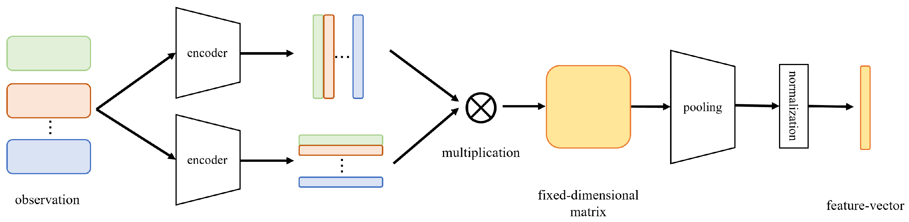
3.1. Variable-Dimensional Observation Processing Network

We propose a deep neural network structure capable of handling variable-dimensional observations. This network can map input observations that undergo changes in specific dimensions to a fixed-dimensional matrix. The network structure leverages the fundamental idea of matrix multiplication. Two matrices can be multiplied if the number of columns in the first matrix is equal to the number of rows in the second matrix., and the shape of multiplication result is independent of the specific dimension. Based on this, we construct two encoders that map the input observations to a high-dimensional feature space along the unchanging dimensions. These two feature matrices will be multiplied across the changeable dimension after mapping. Since both feature matrices are derived from the same observation, their corresponding dimensions are guaranteed to be the same. After completing the matrix multiplication, dimensions of the feature matrices are determined only by the shape of the encoders. The data-flow diagram of the network is shown in Figure 1.

Using a specific situation as an example, consider an input observation $obs\in {\mathbb{R}}^{n\times di{m}_{fixed}}$, where n is variable and $di{m}_{fixed}$ is fixed. Two encoders, $f_1:{\mathbb{R}}^{di{m}_{fixed}}\to {\mathbb{R}}^{di{m}_1}$ are $f_2:{\mathbb{R}}^{di{m}_{fixed}}\to {\mathbb{R}}^{di{m}_2}$, are employed in the neural network structure to process inputs. $di{m}_1$ and $di{m}_2$ are values set as hyper-parameters during the initialization of the neural network and will not change while the network is running. After the input observation undergoes processing by the encoders, the model will output two feature matrices: $f_1\left(obs\right)\in {\mathbb{R}}^{n\times di{m}_1}$ and $f_2\left(obs\right)\in {\mathbb{R}}^{n\times di{m}_2}$. Transpose one of the feature matrices (taking $f_1\left(obs\right)$, for instance) and multiply it with the other feature matrix to obtain the final result $f_{final}\left(obs\right)=f_1^T\left(obs\right)\times f_2\left(obs\right)\in {\mathbb{R}}^{di{m}_1\times n}\times {\mathbb{R}}^{n\times di{m}_2}={\mathbb{R}}^{di{m}_1\times di{m}_2}$. Since the values of $di{m}_1$ and $di{m}_2$ are hyper-parameters, it is implied that the dimension of this result is always fixed, and the dimension of the result can be determined based on the specific tasks.

Additionally, as shown in Figure 1, the input observation undergoes further processing through pooling and normalization layers. The main purpose of the pooling layer is to reduce the dimension of the output, since downstream networks, such as the feature processing network and decision networks, often prefer low-dimensional inputs. The pooling layer is helpful in scenarios where the dimension of the original input is high. The normalization layer aims to standardize the vector after pooling. This operation enhances generalizability of the neural network. Although the network can always process the input observation to a determinant dimension, the value of the output feature matrix increases as the dimension of the input observation increases. Normalization can avoid inconsistency in the output matrix caused by this.

3.2. Decision Networks and Vehicle Simulation Algorithm

The process of driving can be regarded as a Markov decision process (MDP) [47] where the next state of a vehicle only depends on its current state and on the actions it takes in this state. Simulating vehicle behavior essentially involves studying how vehicles choose their actions in specific scenarios. In this paper, we model the decision-making problem during the process of driving as a reinforcement learning problem. As the components of reinforcement learning, the driving scenarios are regarded as the environment;

The behaviors that vehicles can take are considered the action; and the goals of the vehicles are seen as the reward.

We generalize the goals of real-world vehicles into three aspects:

(1)

Purpose: Vehicles typically aim to reach a predefined destination, such as a specific exit at an intersection or a particular location on the road.

(2)

Velocity: Vehicles want to arrive at their destination as quickly as possible by increasing their driving speed.

(3)

Safety: Vehicles always strive to avoid collisions with other vehicles.

These three goals guide the training of vehicle strategies in the simulation through the reward function. Building upon this, the reward function typically consists of three components:

(1)

Purpose reward: If the target vehicle reaches its destination, it will receive the purpose reward.

(2)

Velocity reward: At each timestep, the target vehicle will receive a velocity reward related to its driving speed.

(3)

Collision reward (penalty): If the target vehicle collides with other vehicles, it will incur a collision reward (penalty).

Generally speaking, the purpose reward is assigned a relatively large value, while the velocity reward is relatively small. Since collisions are undesirable, the collision reward is typically represented as a negative value. It should be noted that not every scenario necessarily includes all three types of rewards. The composition of the reward function depends on the specific scenario. For instance, a highway scenario often lacks a purpose reward, while a parking scenario does not provide a velocity reward. Depending on specific conditions, special rewards may also be provided by the environment.

The structure of the decision neural network is shown in Figure 2. As the most value-based reinforcement learning algorithm, we construct a neural network model to estimate the expected rewards for each action that the vehicle can take based on the current observations of the environment. The neural network model consists of the three following components, and the pseudocode for the neural network is presented as Algorithm 1.

(1)

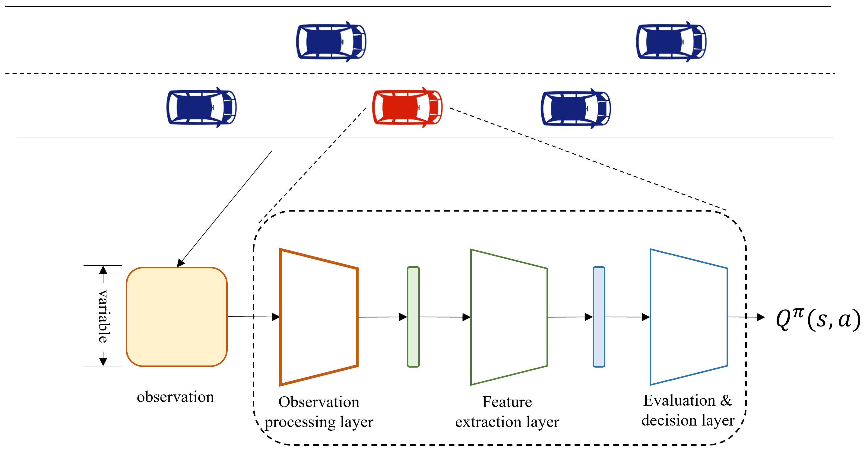
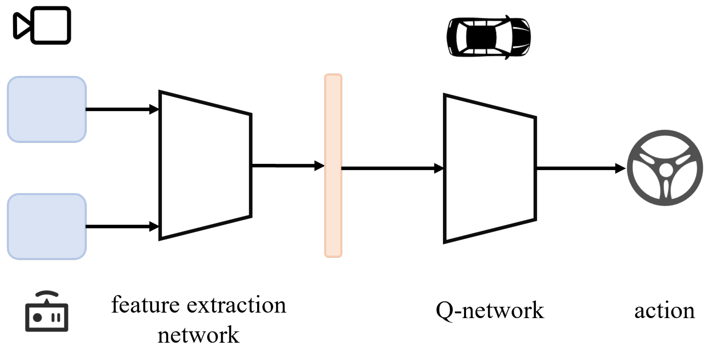
Observation Processing Layer: The purpose of this layer is to map the input observations, which may vary in specific dimensions, to fixed-dimensional feature matrices. The fixed-dimensional matrices will be provided to downstream networks. In this paper, we employ the variable-dimensional observation processing network proposed in Section 3.1.

(2)

Feature Extraction Layer: The aim of the feature extraction layer is to extract the underlying information in the fixed-dimensional feature matrices to assist the downstream network in evaluating the expected rewards. A single-layer linear network is used to achieve this goal.

(3)

Evaluation & Decision Layer: The purpose of this layer is to estimate the reward the vehicle can gain after choosing each action in the current environmental state based on the input features. With the help of value estimation, the vehicle can always greedily select the action with the highest expected reward, in line with the goals encouraged by the rewards. A multi-layer perceptron is employed in this model for evaluating the actions.

Algorithm 1: Deep Neural Network Model
	Data: Current observation of vehicle $obs$
	Result: Estimated value of each action $Q^{\pi }\left(s,a\right)$
1	Initialize the following network: $f_1\left(x\right),f_2\left(x\right):R^{di{m}_1}\to R^{di{m}_{in}}$, $f_{feature}\left(x\right):R^{di{m}_{in}}\to R^{di{m}_{out}}$, $f_Q\left(x\right):R^{di{m}_{out}}\to R^{di{m}_{action}}$;
2	Map observations to the specified feature space: $y_1,y_2=f_1\left(obs\right),f_2\left(obs\right)\in R^{n\times di{m}_{in}}$;
3	Multiply matrices: $y_{fix}=y_1^T{y}_2\in R^{di{m}_{in}\times di{m}_{in}}$. Pool and normalize the fixed-dimensional matrices into input feature vectors: $y_{in}=Norm\left(POO{L}_{mean}\left(y_{fix}\right)\right)\in R^{di{m}_{in}}$;
4	Extract features of input vectors: $y_{out}=f_1\left(y_{in}\right)\in R^{di{m}_{out}}$;
5	Calculate reward expectations for each action through evaluation layer: $Q^{\pi }\left(s,a\right)=f_Q\left(y_{out}\right)\in R^{di{m}_{action}}$

The objective of the whole neural network is to fit the expected reward for each action. Considering that the exact value of cumulative rewards is difficult to obtain, a temporal-difference loss function is used to optimize the neural network, as shown in the Equation (3), where the target value $y_t^{target}=(r_t+ma{x}_{a\in A}{Q}_{t+1}(s_{t+1},a))$ represents the expected cumulative rewards starting from the next state based on the current policy:

$$los{s}_{TD}=\sum _{t=0}^n{[Q_t\left(s_t,a_t\right)-y_t^{target}]}^2.$$

(3)

To avoid the instability caused by the simultaneous updates of estimated value and target value in the loss function, an independent network is used to compute the target values during training. This independent network will not be updated with gradients but rather synchronized with the original network periodically through deep copying.

During the training phase, the neural network receives state inputs from the environment and calculates the expected total rewards for executing each action under the given situation. A separately established target network processes the state inputs of the next timestep, predicting the expected total rewards for executing each action under the next state. Considering that, at each timestep, the vehicle invariably performs an action and receives a single-step reward from the environment as feedback, this reward should approach the difference between the expected total reward for the action taken in the current timestep and the estimated total reward under the best action in the next timestep. This is referred to as the temporal-difference loss function, as shown in Equation (3). The neural network employs the back- algorithm and stochastic gradient descent to update parameters to minimize this difference. This training process is repeated for several rounds until the limit is reached.

Considering the complexity of the traffic system, vehicles are encouraged to choose the most favorable action at each step in trial-and-error learning if they intend to attain the optimal trajectory. This suggests that, in the process of exploring the environment, vehicles should select actions with higher expected rewards to probe for greater rewards.

Unfortunately, when the neural network has not been fully trained, the selection of actions based solely on computed values can pose risks, as there might be a likelihood of being stuck in a local optimal predicament. To address this trade-off, this paper employs $\epsilon$-exploration to enhance the performance of the model. The parameter $\epsilon$ is introduced in the exploration phase. During the exploration phase in the training process, the vehicle stochastically selects actions with a probability of $\epsilon$, otherwise it selects the action with the highest estimated reward. $\epsilon$ is a parameter that decreases over time, starting with a relatively high value to encourage the vehicle to explore the environment at the beginning of training, and decreasing to a lower value in the later stages of training to encourage the vehicle to maximize its rewards.

Additionally, to provide an ample training dataset for the neural network, the experience replay technique is applied in the training process. Instead of being discarded after a single update, each interaction trajectory is stored in an experience replay buffer and repeatedly utilized until the buffer reaches capacity, at which point it is replaced by recent trajectories [48]. The overall pseudo-code for the training of the neural network is presented in Algorithm 2.

Algorithm 2: Training Algorithm for Deep Neural Network
	Data: Simulation environment
	Result: A deep neural network model based on environment
1	#training phase;
2	Initialize the experience replay buffer and parameter $\phi$ of model;
3	while training do
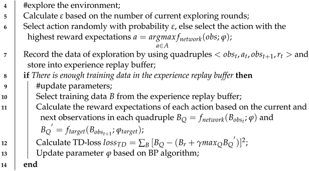15	end

During the simulation phase, we posit the following assumption: at each timestep, the vehicle consistently endeavors to achieve the predefined objectives within the environment, as dictated by the real-world significance of these objectives. Therefore, we prompt the vehicle to select actions greedily by always choosing the action with the highest reward expectations based on the current observation and thereby generating the vehicle’s trajectory within the environment. Considering that the rewards within the environment are provided based on predefined objectives, the more rewards the vehicle obtains, the stronger the consistency between the vehicle’s behavior and the objectives, thus rendering the algorithm rational. The pseudo-code for the simulation algorithm is shown in Algorithm 3.

Algorithm 3: Simulation Algorithm
	Data: Simulation environment
	Result: Simulated trajectory of vehicle
1	Initialize the simulation environment;
2	while This round of simulation has not terminated do
5	end

4. Experiments

4.1. Experimental Environment and Setting

We tested our neural network model and simulation algorithm in the Highway-Env traffic environment simulator (ver1.8.2) [49]. The Highway-Env traffic environment simulator is an open-source environment based on the GYM (ver0.29.1) reinforcement learning environment framework developed by OpenAI [50]. It provides various task scenarios that are reflective of real-world situations. In order to facilitate the smooth operation of our model, the following hyper-parameters were set during the experiments:

(1)

Learning rate: $5\times {10}^{-4}$. The learning rate determines the update extent to the parameters of the neural network at each step based on the loss function during the training process. A higher learning rate leads to larger parameter updates per iteration, making it less likely to get stuck in local optima; however, stability becomes a challenge, and vice versa. To strike a balance, we opted for the value of $5\times {10}^{-4}$ which is commonly used in most reinforcement learning models.

(2)

Replay buffer capacity: 15,000. The capacity of the replay buffer determines the number of tuples it can store. When the number of stored tuples reaches the limit, the earliest data in the buffer are replaced by the most recently obtained data. A larger capacity means data can be stored in the buffer for a longer interval. This provides a greater quantity of diverse data but also leads to lower policy consistency, and vice versa. Since the value-based methods employed in this paper require a considerable amount of data for training and necessitate diverse data for a comprehensive environmental assessment, we chose a larger capacity for the replay buffer.

(3)

Discount factor: 0.8. The discount factor determines the model’s emphasis on future rewards. A higher discount factor means that future rewards have a larger value at the current timestep, indicating a greater emphasis on future rewards, and vice versa. The traffic simulation problem can be considered a Markov decision process with evenly distributed rewards. Vehicles should focus more on the reward of the current timestep. To achieve this goal, a relatively lower discount factor should be selected.

(4)

Target network update interval: 50. The target network update interval determines the frequency at which the target network synchronizes with the source network. A larger interval leads to a lower synchronization frequency, resulting in more stable training but also in poorer consistency between the target and source networks, and vice versa. With the aim of balancing stability and consistency during the training process, the update interval is set to a moderately averaged value.

We constructed our deep neural network model and simulation algorithm using the open-source machine learning package PyTorch (ver11.8), which is based on python (ver3.8). To ensure the fairness of our results, we employed Stable-Baselines3 (ver2.1) [51] as the baseline for reinforcement learning. The code was deployed on a server equipped with an Intel i9-13900KF processor made in Chinese Mainlandand NVIDIA GeForce RTX 4090 made in Chinese Mainland for computation.

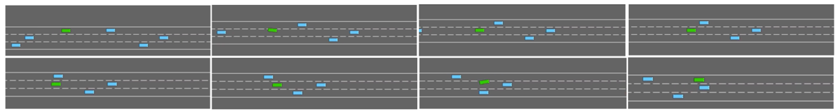
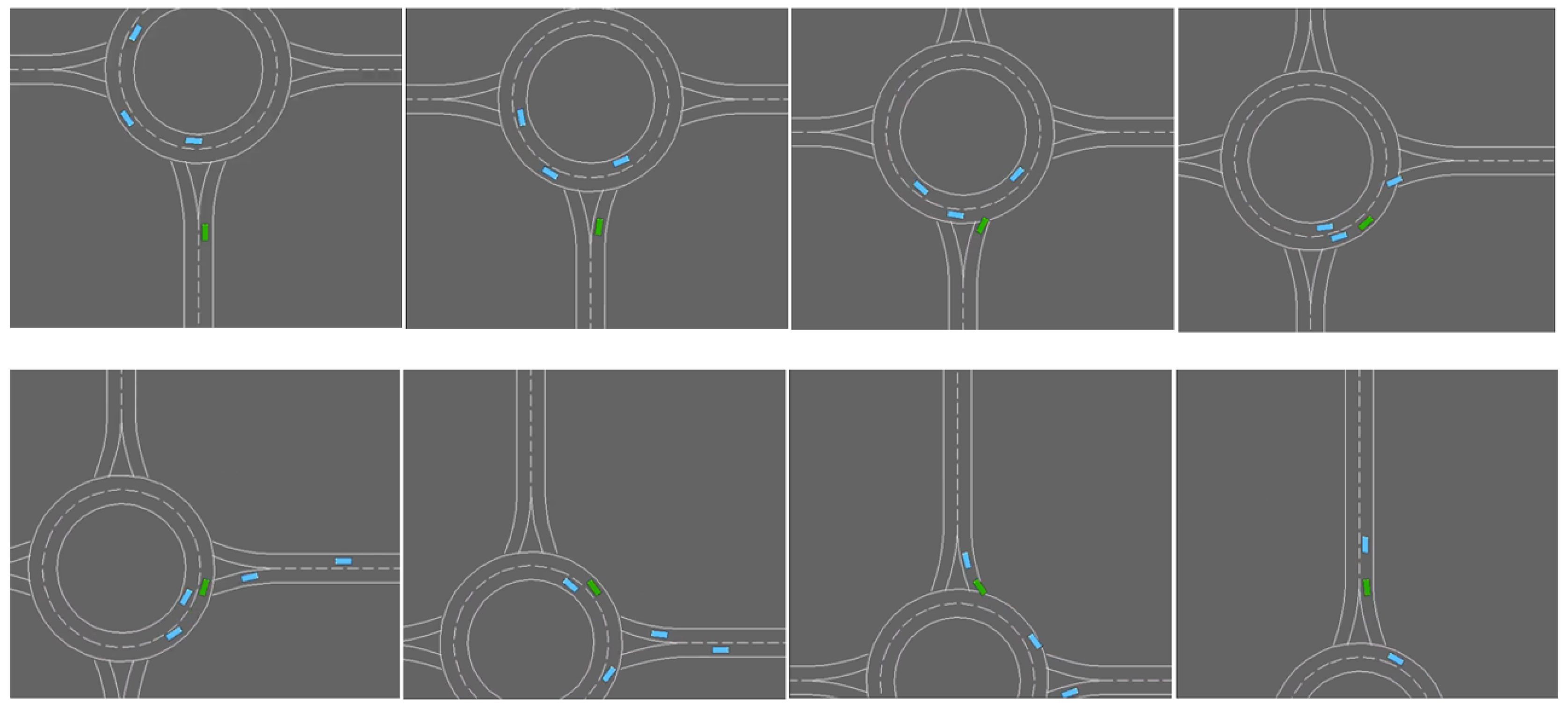
4.2. Feasibility Verification

In this section, we select two highly representative real-world scenarios, highway driving and roundabout navigation, to validate the feasibility of our model in practical situations. In both scenarios, the traffic environment simulator generates a vehicle controlled by a reinforcement learning neural network and several vehicles controlled by predefined non-heuristic algorithms within the simulator. At each timestep of the simulation, the neural network is required to select one and only one action from the simulator’s predefined meta actions—➀ accelerate, ➁ maintain speed, ➂ decelerate, ➃ change lane left, and ➄ change lane right—and to interact with the environment. The details of each environment are as follows. In the interest of fairness, the reward values were configured using the default settings provided by the simulator.

Highway driving: The simulator provides a road system consisting of several straight lanes. The vehicle controlled by the neural network starts from one side of the road and travels toward the other side. The road is long enough that the simulation is focused on the vehicle’s driving process without a destination. In this scenario, the vehicle is encouraged to drive at a high speed as much as possible. The vehicle will receive a velocity reward proportional to the driving speed, with the maximum velocity reward of 0.4 achieved at the maximum allowable speed. In the real world, vehicles are encouraged to be in the rightmost lane, i.e., the carriageway. Therefore, if the vehicle is in the rightmost lane, it will receive a special reward of 0.1. Collisions with other vehicles are strictly to be avoided. If a collision occurs during driving, the simulator will provide a negative reward of $-1$ and forcibly shut down the current simulation. The total reward for the vehicle at each timestep is the sum of the mentioned rewards.

Roundabout navigation: The simulator provides a roundabout system consisting of two circular lanes and three exits. The vehicle controlled by the neural network enters the roundabout from a specified entrance and exits from another specified exit. As the target exit of the reinforcement learning vehicle may not always be the same as that of other vehicles, the vehicle must learn to avoid collisions with exiting vehicles. In this scenario, high-speed driving is mildly encouraged, and the vehicle will be rewarded proportionally to its driving speed, with a maximum velocity reward of 0.2 at maximum speed. A collision with another vehicle results in a negative reward of $-1$ and shuts down the current simulation. Furthermore, from the perspective of traffic regulations, changing lanes within the roundabout is considered to be an unsupervised behavior. It may cause difficulties for other vehicles on the road. Therefore, whenever the vehicle selects the “change lane” action, the simulator will provide a negative reward of $-0.05$. The total reward for the vehicle at each timestep is the sum of the mentioned rewards.

As an essential basis for determining the selected actions of the vehicle and as the input for the reinforcement learning neural network, the simulator provides observations at the current time to the neural network at each timestep. In the aforementioned two scenarios, the observations consist of the states of vehicles closest to the reinforcement learning vehicle. The state of each vehicle comprises five elements: x, y, $v_x$, $v_y$, and $presence$. x and y represent the lateral and longitudinal coordinates of the vehicle, while $v_x$ and $v_y$ represent the vehicle’s lateral and longitudinal velocities. The $presence$ element is a special mask, and its value is usually 1. However, when the number of vehicles within the observation range is less than the capacity of the observation, a state with coordinates and velocities both set to 0 will be used to fill the observation. In this situation, $presence$ will be set to 0 to indicate that the corresponding observation is invalid. As a central aspect of this paper, we seek to verify the ability of the designed neural network to handle observations with variable dimensions. Therefore, the highway driving scenario is configured to observe the closest four vehicles, while the roundabout navigation scenario is configured to observe the closest five vehicles. This means the observation dimensions are 4 × 5 for the highway scenario and 5 × 5 for the roundabout scenario. We deployed the neural network and simulation algorithm in the simulator consistent with the pseudocode. Considering the small data scale and medium complexity within the simulation environment, as well as the limit of computational resources, we opted for a moderate hidden layer dimension of 256. The parameter dimensions of each layer of the neural network are shown in

Table 1. Parameter dimensions of each layer.

Layer	Name	Dimension	Activation Function
Observation Processing Layer	$f_1\left(x\right)$	$5\times 256$	ReLU
	$f_2\left(x\right)$	$5\times 256$	ReLU
Feature Extraction Layer	$f_{feature}\left(x\right)$	$256\times 256$	ReLU
Evaluation & Decision Layer	$f_Q\left(x\right)$	$256\times 5$	-

. It should be clarified that the Rectified Linear Unit (ReLU) activation function is employed to further process the output values by the network. This is aimed at circumventing the issue of gradient vanishing in multi-layer neural networks. Concurrently, the ReLU activation function is linear only within the positive domain, while it remains constant at zero within the negative domain, resulting in a sparse representation in the network, which aids in better learning of the distinctive features. The efficacy of this activation function has been validated in several successful research works [52,53].

The neural network is trained for 10,000 timesteps in each scenario of the simulator, and it generated replays using the trained neural network for simulation. Figure 3 presents eight snapshots of the highway scenario simulation. In this simulation, the reinforcement learning vehicle (indicated in green) is driving in the way. In order to maintain a relatively high speed, when encountering slower vehicles (depicted in blue), the reinforcement learning vehicle overtakes by changing lanes twice successively and then returns to the original lane to continue its journey. Figure 4 displays eight snapshots of the roundabout scenario simulation. In this simulation, the reinforcement learning vehicle (indicated in green) adeptly controlled its speed to avoid collisions with other vehicles (indicated in blue) upon entering the roundabout and passing the first exit (non-target exit), and then exited correctly at the second exit (target exit). The simulation snapshots demonstrate that the neural network designed in this paper is capable of handling observations of varying dimensions using a fixed-size neural network and ultimately achieves consistent simulation results with the scenario objectives, thereby proving its feasibility.

4.3. Comparative Analysis

The neural network designed in this paper is an advancement on the deep Q-Learning network, achieved by devising a fixed-shape network that endows the model with the ability to handle observations of variable dimensions. However, the process of observation requires careful validation, as improper processes may result in information loss and lead to a decline in model performance. This concern is also present in the network designed in this paper. In order to verify that the process of transforming variable-dimensional observations into fixed-dimensional features does not lead to the loss of information in observation, we additionally deployed a baseline network using only the deep Q-Learning network in the experimental environment. In the baseline network, the input observations are reshaped into column vectors without any processing. The deep Q-Learning network is incapable of handling inputs of various dimensions. Therefore, we separately configured and trained feature extractors for each scenario to provide the deep Q-Learning network with fixed-dimensional features. The parameter dimensions of the deep Q-Learning network used are shown in

Table 2. Parameter dimensions of each layer (deep Q-Learning network).

Layer	Name	Dimension	Activation Function
Feature Extraction Layer	$f_{feature}\left(x\right)$	$di{m}_{obs}\times 256$	ReLU
	$f_2\left(x\right)$	$256\times 256$	ReLU
Evaluation & Decision Layer	$f_Q\left(x\right)$	$256\times 5$	-

, where $di{m}_{obs}$ represents the current observation dimension and varies across scenarios.

To more comprehensively demonstrate the contrast in training phases between our neural network and the deep Q-Learning network, we introduced two additional scenarios in the simulator for testing purposes: merge junction and U-shaped lane. Both the merge junction and U-shaped lane scenarios focus on the process of driving on roadways. The merge junction scenario consists of two straight lanes and one merging lane, as shown in Figure 5a. The reinforcement learning vehicle departs from one side of the straight lane and needs to learn how to handle merging vehicles during its process of driving, enabling itself to travel at higher speeds without colliding with other vehicles. In the merge junction scenario, the total reward comprises a velocity reward proportional to the speed, with a maximum value of 0.2; a 0.1 reward for traveling in the right lane; a −1 collision penalty; and a −0.05 lane change penalty. The U-shaped lane consists of two lanes shaped similarly to the letter “U”, as shown in Figure 5b. The reinforcement learning vehicle must learn to handle overtaking and lane cruising, especially during turning. The total reward in the U-shaped lane scenario includes a velocity reward proportional to the speed, with a maximum value of 0.4; a 0.1 reward for traveling in the inner lane; and a −1 collision penalty.

We conducted experiments on the neural network designed in this paper and the deep Q-Learning network serving as the baseline for 10,000 timesteps each and collected their rewards obtained during the training process, as shown in Figure 6. The reward reflects the consistency between the action of the reinforcement learning vehicle and the objectives, thus serving as an indicator of the model’s performance. The trend depicted in the figure illustrates that training efficiency of our method is not inferior to that of the deep Q-Learning network in those scenarios. This indicates that our observation processing network does not compromise the quality of the resulting features and represents a method that can be practically applied.

5. Conclusions and Discussion

In this paper, we designed a neural network model based on reinforcement learning that is capable of handling variable-dimensional observation with a fixed network shape to accommodate the differences in observation dimensions offered by various real-world traffic systems. Correspondingly, we propose a neural network training algorithm and a vehicle simulation algorithm based on the neural network. Our method circumvents the strict limitations on input dimensions inherent to the mathematical nature of neural networks, thereby facilitating the application of reinforcement learning methods with excellent data processing capabilities to a broader range of vehicle simulation tasks.

Our method exhibits strong scalability. Our primary contribution lies in the design of the neural network that maps input observation with variable dimensions to fixed-dimensional feature matrices. From the perspective of structure, the neural network represents a transformation of the feature, signifying compatibility with other feature processing methods. Feature processing methods such as attention mechanisms and recurrent neural networks can be employed to reinforce fixed-dimensional feature vectors. In particular, dimension-independent feature processing methods like convolutional neural networks can also be applied to handle variable-dimensional observations. This adaptability allows our framework to accommodate prospective feature processing methods, thereby achieving superior performance.

From an application standpoint, our method can likewise be implemented in the vehicle-control problem. This is due to our method of mapping the present state into actions, which is also the solution to the vehicle-control problem. In this situation, the input for the network would be supplied by the real-world environment instead of a simulator. Real-world information is primarily gathered via onboard devices such as cameras and sensors. The data provided by these devices comprise environmental snapshots, which are differ from the detailed environmental information offered by simulators. Therefore, a pretrained feature extraction network is recommended to process the data before data is fed into the Q-network. The Q-network can be designed as discussed in Section 3, and data can be converted into value estimations. In practice, the Q-network employed could either be a pretrained one with fixed parameters or a pretrained neural network that is fine-tuned through imitation learning. Nevertheless, the use of untrained neural networks is strongly discouraged due to the unacceptable cost of trial-and-error in the real-world. Once the action is selected, given that the vehicle interacts with the real world via mechanical devices such as wheels, the Q-network would need to be connected to an external controller to enact the selected actions in the real world. Figure 7 illustrates a schematic representation of how our method can be deployed in vehicular control problems. In fact, there have already been some studies attempting to use reinforcement learning methods for vehicle control [54,55], but their network structures differ from the method in this paper.

In future work, considering that this paper is based on observations that vary across a specific dimension, an important question pertains to how to extend the network’s structure so that it can be applied to observations that may vary across other dimensions. Furthermore, a potential method that needs further exploration lies in model transfer and generalization [56]. Historically, the transfer of neural network models from one environment to another without excessive loss of performance has been a focal point for reinforcement learning researchers [57]. Excellent transfer algorithms enable models to perform well across multiple scenarios while reducing training time and storage cost. In real-world traffic scenarios, vehicles may encounter highly variable situations. Neural network models that can adapt to diverse environments are of paramount importance in vehicle simulation tasks. The present work enables models to perform adequately across multiple scenarios, even when the offered dimensions of observation differ. Such models provide a prerequisite for cross-scenario research, including investigations about parameter sharing [58], knowledge representation [59], and related issues. Building upon this work, methods such as environment modeling and representation learning can be integrated into the model to assist in making targeted decisions across different environments. Moreover, the ultimate strategy of reinforcement learning is highly correlated with the environment used. Consequently, from the perspective of the real-world, constructing simulators for reinforcement learning that closely align with real-world situations is a task deserving attention in future research, aiming to aid models in learning decisions applicable to real-world scenarios. For instance, even though scenarios with multiple round lines and exits in a roundabout environment exhibit some homogeneity with those involving two round lines and three exits, they still show differences in numerous subtle aspects. Implementing simulations of such scenarios in the simulator and deploying simulation algorithms for this set of conditions constitute a research endeavor worth pursuing.

References

- Dawood, N.N.; Castro, S.S. Automating road construction planning with a specific-domain simulation system. J. Inf. Technol. Constr. 2009, 1, 556–573. [Google Scholar]
- Gambardella, L.M.; Rizzoli, A.E.; Funk, P. Agent-based planning and simulation of combined rail/road transport. Simulation 2002, 78, 293–303. [Google Scholar] [CrossRef]
- Wang, J.; Yan, Y.; Zhang, K.; Chen, Y.; Cao, M.; Yin, G. Path planning on large curvature roads using driver-vehicle-road system based on the kinematic vehicle model. IEEE Trans. Veh. Technol. 2021, 71, 311–325. [Google Scholar] [CrossRef]
- Aycin, M.; Benekohal, R. Comparison of car-following models for simulation. Transp. Res. Rec. 1999, 1678, 116–127. [Google Scholar] [CrossRef]
- Li, Y.; Sun, D. Microscopic car-following model for the traffic flow: The state of the art. J. Control Theory Appl. 2012, 10, 133–143. [Google Scholar] [CrossRef]
- Wang, J.; Lv, W.; Jiang, Y.; Qin, S.; Li, J. A multi-agent based cellular automata model for intersection traffic control simulation. Phys. A Stat. Mech. Its Appl. 2021, 584, 126356. [Google Scholar] [CrossRef]
- Krajzewicz, D.; Brockfeld, E.; Mikat, J.; Ringel, J.; Rössel, C.; Tuchscheerer, W.; Wagner, P.; Wösler, R. Simulation of modern traffic lights control systems using the open source traffic simulation SUMO. In Proceedings of the 3rd Industrial Simulation Conference 2005, EUROSIS-ETI, Berlin, Germany, 9–11 June 2005; pp. 299–302. [Google Scholar]
- Gipps, P.G. A behavioural car-following model for computer simulation. Transp. Res. Part B Methodol. 1981, 15, 105–111. [Google Scholar] [CrossRef]
- Koukounaris, A.I.; Stephanedes, Y.J. Connected Intelligent Transportation System Model to Minimize Societal Cost of Travel in Urban Networks. Sustainability 2023, 15, 15383. [Google Scholar] [CrossRef]
- Zhao, X.M.; Gao, Z.Y. A new car-following model: Full velocity and acceleration difference model. Eur. Phys. J. B-Condens. Matter Complex Syst. 2005, 47, 145–150. [Google Scholar] [CrossRef]
- Saifuzzaman, M.; Zheng, Z. Incorporating human-factors in car-following models: A review of recent developments and research needs. Transp. Res. Part C Emerg. Technol. 2014, 48, 379–403. [Google Scholar] [CrossRef]
- Ranjitkar, P.; Nakatsuji, T.; Kawamua, A. Car-following models: An experiment based benchmarking. J. East. Asia Soc. Transp. Stud. 2005, 6, 1582–1596. [Google Scholar]
- Shokri, D.; Larouche, C.; Homayouni, S. A Comparative Analysis of Multi-Label Deep Learning Classifiers for Real-Time Vehicle Detection to Support Intelligent Transportation Systems. Smart Cities 2023, 6, 2982–3004. [Google Scholar] [CrossRef]
- Wang, X.; Yang, Z.; Feng, H.; Zhao, J.; Shi, S.; Cheng, L. A Multi-Stream Attention-Aware Convolutional Neural Network: Monitoring of Sand and Dust Storms from Ordinary Urban Surveillance Cameras. Remote Sens. 2023, 15, 5227. [Google Scholar] [CrossRef]
- Alsrehin, N.O.; Gupta, M.; Alsmadi, I.; Alrababah, S.A. U2-Net: A Very-Deep Convolutional Neural Network for Detecting Distracted Drivers. Appl. Sci. 2023, 13, 11898. [Google Scholar] [CrossRef]
- Wang, N.; Zhang, B.; Gu, J.; Kong, H.; Hu, S.; Lu, S. Urban Road Traffic Spatiotemporal State Estimation Based on Multivariate Phase Space–LSTM Prediction. Appl. Sci. 2023, 13, 12079. [Google Scholar] [CrossRef]
- Jin, Z.; Noh, B. From prediction to prevention: Leveraging deep learning in traffic accident prediction systems. Electronics 2023, 12, 4335. [Google Scholar] [CrossRef]
- Bowman, L.A.; Narayanan, R.M.; Kane, T.J.; Bradley, E.S.; Baran, M.S. Vehicle Detection and Attribution from a Multi-Sensor Dataset Using a Rule-Based Approach Combined with Data Fusion. Sensors 2023, 23, 8811. [Google Scholar] [CrossRef]
- Manderna, A.; Kumar, S.; Dohare, U.; Aljaidi, M.; Kaiwartya, O.; Lloret, J. Vehicular Network Intrusion Detection Using a Cascaded Deep Learning Approach with Multi-Variant Metaheuristic. Sensors 2023, 23, 8772. [Google Scholar] [CrossRef]
- Liu, G.; He, S.; Han, X.; Luo, Q.; Du, R.; Fu, X.; Zhao, L. Self-Supervised Spatiotemporal Masking Strategy-Based Models for Traffic Flow Forecasting. Symmetry 2023, 15, 2002. [Google Scholar] [CrossRef]
- Zhu, M.; Wang, X.; Wang, Y. Human-like autonomous car-following model with deep reinforcement learning. Transp. Res. Part C Emerg. Technol. 2018, 97, 348–368. [Google Scholar] [CrossRef]
- Wei, H.; Zheng, G.; Yao, H.; Li, Z. Intellilight: A reinforcement learning approach for intelligent traffic light control. In Proceedings of the 24th ACM SIGKDD International Conference on Knowledge Discovery & Data Mining, London, UK, 19–23 August 2018; pp. 2496–2505. [Google Scholar]
- Chinchali, S.; Hu, P.; Chu, T.; Sharma, M.; Bansal, M.; Misra, R.; Pavone, M.; Katti, S. Cellular network traffic scheduling with deep reinforcement learning. In Proceedings of the AAAI Conference on Artificial Intelligence, New Orleans, LA, USA, 2–7 February 2018; Volume 32. [Google Scholar]
- François-Lavet, V.; Henderson, P.; Islam, R.; Bellemare, M.G.; Pineau, J. An introduction to deep reinforcement learning. Found. Trends® Mach. Learn. 2018, 11, 219–354. [Google Scholar] [CrossRef]
- Henderson, P.; Islam, R.; Bachman, P.; Pineau, J.; Precup, D.; Meger, D. Deep reinforcement learning that matters. In Proceedings of the AAAI Conference on Artificial Intelligence, New Orleans, LA, USA, 2–7 February 2018; Volume 32. [Google Scholar]
- Dai, X.; Li, C.K.; Rad, A.B. An approach to tune fuzzy controllers based on reinforcement learning for autonomous vehicle control. IEEE Trans. Intell. Transp. Syst. 2005, 6, 285–293. [Google Scholar] [CrossRef]
- Yurtsever, E.; Lambert, J.; Carballo, A.; Takeda, K. A survey of autonomous driving: Common practices and emerging technologies. IEEE Access 2020, 8, 58443–58469. [Google Scholar] [CrossRef]
- Liu, L.; Lu, S.; Zhong, R.; Wu, B.; Yao, Y.; Zhang, Q.; Shi, W. Computing systems for autonomous driving: State of the art and challenges. IEEE Internet Things J. 2020, 8, 6469–6486. [Google Scholar] [CrossRef]
- Liu, H.; Kiumarsi, B.; Kartal, Y.; Taha Koru, A.; Modares, H.; Lewis, F.L. Reinforcement learning applications in unmanned vehicle control: A comprehensive overview. Unmanned Syst. 2023, 11, 17–26. [Google Scholar] [CrossRef]
- Ma, X.; Driggs-Campbell, K.; Kochenderfer, M.J. Improved robustness and safety for autonomous vehicle control with adversarial reinforcement learning. In Proceedings of the 2018 IEEE Intelligent Vehicles Symposium (IV), Changshu, China, 26–30 June 2018; pp. 1665–1671. [Google Scholar]
- Alghodhaifi, H.; Lakshmanan, S. Autonomous vehicle evaluation: A comprehensive survey on modeling and simulation approaches. IEEE Access 2021, 9, 151531–151566. [Google Scholar] [CrossRef]
- Yang, Q.I.; Koutsopoulos, H.N. A microscopic traffic simulator for evaluation of dynamic traffic management systems. Transp. Res. Part C Emerg. Technol. 1996, 4, 113–129. [Google Scholar] [CrossRef]
- Adams, S.; Yu, L. An Evaluation of Traffic Simulation Models for Supporting Its Development; Technical Report; Center for Transportation Training and Research, Texas Southern University: Houston, TX, USA, 2000. [Google Scholar]
- Ruskin, H.J.; Wang, R. Modeling traffic flow at an urban unsignalized intersection. In Proceedings of the Computational Science—ICCS 2002: International Conference, Amsterdam, The Netherlands, 21–24 April 2002; Springer: Berlin/Heidelberg, Germany, 2002; pp. 381–390. [Google Scholar]
- Reece, D.A.; Shafer, S.A. A computational model of driving for autonomous vehicles. Transp. Res. Part A Policy Pract. 1993, 27, 23–50. [Google Scholar] [CrossRef]
- Sutton, R.S.; Barto, A.G. Reinforcement Learning: An Introduction; MIT Press: Cambridge, MA, USA, 1998; Volume 22447. [Google Scholar]
- Russell, S.J.; Norvig, P. Artificial Intelligence a Modern Approach; Prentice Hall: London, UK, 2010. [Google Scholar]
- Puterman, M.L. Markov Decision Processes: Discrete Stochastic Dynamic Programming; John Wiley & Sons: Hoboken, NJ, USA, 2014. [Google Scholar]
- Schulman, J.; Wolski, F.; Dhariwal, P.; Radford, A.; Klimov, O. Proximal policy optimization algorithms. arXiv 2017, arXiv:1707.06347. [Google Scholar]
- Mnih, V.; Kavukcuoglu, K.; Silver, D.; Graves, A.; Antonoglou, I.; Wierstra, D.; Riedmiller, M. Playing atari with deep reinforcement learning. arXiv 2013, arXiv:1312.5602. [Google Scholar]
- Bellman, R. On the theory of dynamic programming. Proc. Natl. Acad. Sci. USA 1952, 38, 716–719. [Google Scholar] [CrossRef] [PubMed]
- Whiteson, S. A Theoretical and Empirical Analysis of Expected Sarsa. In Proceedings of the 2009 IEEE Symposium on Adaptive Dynamic Programming and Reinforcement Learning, Nashville, TN, USA, 30 March–2 April 2009. [Google Scholar]
- Watkins, C.J.C.H. Learning from Delayed Rewards. Ph.D. Thesis, Cambridge University, Cambridge, UK, 1989. [Google Scholar]
- Mnih, V.; Kavukcuoglu, K.; Silver, D.; Rusu, A.A.; Veness, J.; Bellemare, M.G.; Graves, A.; Riedmiller, M.; Fidjeland, A.K.; Ostrovski, G.; et al. Human-level control through deep reinforcement learning. Nature 2015, 518, 529–533. [Google Scholar] [CrossRef] [PubMed]
- Hausknecht, M.; Stone, P. Deep recurrent q-learning for partially observable mdps. In Proceedings of the 2015 AAAI Fall Symposium Series, Arlington, VA, USA, 12–14 November 2015. [Google Scholar]
- Tesauro, G. Temporal difference learning and TD-Gammon. Commun. ACM 1995, 38, 58–68. [Google Scholar] [CrossRef]
- Hu, Q.; Yue, W. Markov Decision Processes with Their Applications; Springer Science & Business Media: Berlin/Heidelberg, Germany, 2007; Volume 14. [Google Scholar]
- Schaul, T.; Quan, J.; Antonoglou, I.; Silver, D. Prioritized experience replay. arXiv 2015, arXiv:1511.05952. [Google Scholar]
- Leurent, E. An Environment for Autonomous Driving Decision-Making. 2018. Available online: https://github.com/eleurent/highway-env (accessed on 28 April 2018).
- Brockman, G.; Cheung, V.; Pettersson, L.; Schneider, J.; Schulman, J.; Tang, J.; Zaremba, W. OpenAI Gym. arXiv 2016, arXiv:1606.01540. [Google Scholar]
- Raffin, A.; Hill, A.; Gleave, A.; Kanervisto, A.; Ernestus, M.; Dormann, N. Stable-Baselines3: Reliable Reinforcement Learning Implementations. J. Mach. Learn. Res. 2021, 22, 12348–12355. [Google Scholar]
- Sunehag, P.; Lever, G.; Gruslys, A.; Czarnecki, W.M.; Zambaldi, V.; Jaderberg, M.; Lanctot, M.; Sonnerat, N.; Leibo, J.Z.; Tuyls, K.; et al. Value-decomposition networks for cooperative multi-agent learning. arXiv 2017, arXiv:1706.05296. [Google Scholar]
- Rashid, T.; Samvelyan, M.; De Witt, C.S.; Farquhar, G.; Foerster, J.; Whiteson, S. Monotonic value function factorisation for deep multi-agent reinforcement learning. J. Mach. Learn. Res. 2020, 21, 7234–7284. [Google Scholar]
- Pan, X.; You, Y.; Wang, Z.; Lu, C. Virtual to real reinforcement learning for autonomous driving. arXiv 2017, arXiv:1704.03952. [Google Scholar]
- Kiran, B.R.; Sobh, I.; Talpaert, V.; Mannion, P.; Al Sallab, A.A.; Yogamani, S.; Pérez, P. Deep reinforcement learning for autonomous driving: A survey. IEEE Trans. Intell. Transp. Syst. 2021, 23, 4909–4926. [Google Scholar] [CrossRef]
- Taylor, M.E.; Stone, P. Transfer learning for reinforcement learning domains: A survey. J. Mach. Learn. Res. 2009, 10, 1633–1685. [Google Scholar]
- Da Silva, F.L.; Costa, A.H.R. A survey on transfer learning for multiagent reinforcement learning systems. J. Artif. Intell. Res. 2019, 64, 645–703. [Google Scholar] [CrossRef]
- Kaushik, M.; Singhania, N.; Krishna, K.M. Parameter sharing reinforcement learning architecture for multi agent driving. In Proceedings of the Advances in Robotics, Chennai, India, 2–6 July 2019; pp. 1–7. [Google Scholar]
- Comanici, G.; Precup, D.; Barreto, A.; Toyama, D.K.; Aygün, E.; Hamel, P.; Vezhnevets, S.; Hou, S.; Mourad, S. Knowledge Representation for Reinforcement Learning Using General Value Functions. 2018; openreview. [Google Scholar]