Abstract
Effective vehicle detection plays a crucial role in various applications in cities, including traffic management, urban planning, vehicle transport, and surveillance systems. However, existing vehicle detection methods suffer from low recognition accuracy, high computational costs, and excessive parameters. To address these challenges, this paper proposed a high-precision and lightweight detector along with a new dataset for construction-related vehicles. The dataset comprises 8425 images across 13 different categories of vehicles. The detector was based on a modified version of the You Only Look Once (YOLOv4) algorithm. DenseNet was utilized as the backbone to optimize feature transmission and reuse, thereby improving detection accuracy and reducing computational costs. Additionally, the detector employed depth-wise separable convolutions to optimize the model structure, specifically focusing on the lightweight neck and head components. Furthermore, H-swish was used to enhance non-linear feature extraction. The experimental results demonstrated that the proposed detector achieves a mean average precision (mAP) of 96.95% on the provided dataset, signifying a 4.03% improvement over the original YOLOv4. The computational cost and parameter count of the detector were 26.09GFLops and 16.08 MB, respectively. The proposed detector not only achieves lower computational costs but also provides higher detection when compared to YOLOv4 and other state-of-the-art detectors.
1. Introduction
In recent years, the urban area has experienced continuous expansion, characterized by a rising number of construction activities and vehicles in the city. The rapid development of cities has presented great challenges for urban traffic management [1,2]. Therefore, accurate vehicle detection in cities is particularly important and indispensable for urban traffic management and facility construction [3,4].
During the initial stages, vehicle detection mainly relied on machine learning and digital image processing technology [5]. These methods utilize digital image processing technology to extract vehicle-related features (e.g., edges, colors, textures, etc.) from the image, and combine machine learning algorithms (e.g., support vector machine (SVM), random forest, and AdaBoost) to recognize vehicles [6,7]. Nevertheless, despite achieving some success, these early approaches are typically susceptible to image quality, lighting conditions, and changes in perspective. Therefore, their application in complex scenes is relatively limited.
Recently, there has been a significant advancement in vehicle detection methods with the emergence of deep learning and convolutional neural networks (CNNs) [8,9,10]. These methods not only enable end-to-end vehicle recognition but also have higher detection accuracy. Furthermore, they can handle more complex visual tasks [11]. Nevertheless, existing vehicle detection methods typically encounter challenges, such as high computational costs, low detection accuracy, and large model parameters [12]. In addition, vehicle detection also confronts the problem of the limited availability of image datasets.
To address these problems, this paper proposes a high-precision and lightweight vehicle detector for construction-related vehicles, aiming to improve traffic management and urban planning. The detector not only achieves high detection accuracy but also significantly reduces the number of parameters and computational costs. This vehicle detector aims to provide an efficient and practical solution for the planning and management of real-world cities.
Furthermore, to address the scarcity of vehicle datasets and support the development and evaluation of the proposed detector, a new construction-related vehicle dataset was proposed. This dataset includes 8425 images across 13 categories of vehicles in both building construction and non-construction scenes. This dataset can provide comprehensive training and testing for various popular and advanced detectors, enabling a comprehensive evaluation of their vehicle detection performance in urban environments.
The proposed vehicle detector was built upon the widely acclaimed YOLOv4 algorithm [8], which has exhibited excellent performance in object detection tasks. To enhance its performance in urban vehicle detection, several modifications were performed. Notably, by utilizing DenseNet121 [13] as the backbone network and leveraging its unique dense connection mechanism, the feature extraction capability of the detector has been improved. This optimization enhances feature transmission and reuse, thereby improving detection accuracy while minimizing computational costs. In addition, depth-wise separable convolution [14] was incorporated into the detection framework to the lightweight neck and head to optimize the structure of the detector. This optimization not only improved the efficiency of the model but also reduced the number of parameters and computational costs. Moreover, the H-Swish activation function [15] was incorporated to facilitate better non-linear feature extraction, contributing to an improved detection accuracy of vehicles in urban environments. The key contributions of this paper are summarized as follows:
- We proposed a new high-precision and lightweight vehicle detector. The detector utilizes Densenet121 as the backbone network, greatly improving feature transmission and reuse. Additionally, depth-wise separable convolution was introduced outside the backbone network to reduce computational costs and the number of parameters. Moreover, we employed the H-Swish function to enhance non-linear feature extraction.
- We proposed a new image dataset comprising 8425 images across 13 different categories of vehicles for the detection of construction-related vehicles. The dataset solves the problem of limited availability of image datasets for construction-related vehicles.
- We performed a series of experiments using 17 popular SOTA detection models on the proposed dataset. The experimental results revealed that the proposed detector achieves higher detection accuracy, lower computational costs, and fewer parameters than other detection models.
The subsequent sections of this paper are organized as follows: Section 2 presents an in-depth review of related work in vehicle detection, highlighting the limitations of existing methods. Section 3 provides a detailed description of the methodology employed in the proposed high-precision and lightweight vehicle detector. Section 4 outlines the dataset. Section 5 introduces the experimental settings and evaluation metrics. The results and analysis are presented in Section 6. Finally, Section 7 concludes this work.
2. Related Work
Vehicle detection in urban environments has been an active research area, with numerous methods proposed to tackle the challenges associated with accurate and efficient detection. In this section, we review the existing literature and analyze the limitations of current methods.
2.1. Methods Based on Digital Image Processing and Machine Learning
In the early days, many methods based on digital image processing and machine learning were used to accurately detect vehicles in cities [16,17]. To address these issues, a method based on the Kalman filter was proposed [18]. This approach employs edge detection and blob detection to extract the centroid and bounding box features of the detected objects. The Kalman filter algorithm was then utilized in the tracking process to enhance the accuracy of target detection and position prediction. To overcome the challenge of detecting vehicles with varying sizes, a method was introduced in [19], involving the initial detection of moving vehicles using optical flow, followed by the application of a shadow detection algorithm based on the hue, saturation, and value color space and a region labeling algorithm for shadow removal, ensuring the accurate detection of moving vehicles. Additionally, for improved vehicle counting, a method based on the combination of HSV color distance and centroid distance has been proposed [20]. Furthermore, to achieve precise vehicle tracking, a novel vehicle detection and tracking approach has been presented in [21]. This method utilizes the generic invariant spatial–temporal (GIST) image processing algorithm and a support vector machine (SVM) classifier, extracting vehicle features from images or video data acquired through sensors installed on board the vehicle, and employing edge feature matching and a Kalman filter for the tracking process. To enhance the accuracy of vehicle detection, methods based on feature extraction using techniques such as the histogram of oriented gradient (HOG) method [22], Haar-like features [23], and local binary patterns (LBPs) [24] have been proposed. To further improve the robustness and generalization of vehicle recognition, methods employing machine learning algorithms, such as artificial neural networks [25], Adaboost [26,27], random forest [28], and naïve Bayes [29], have also been introduced.
However, these methods still face several challenges, including sensitivity to changes in lighting conditions, difficulty in handling complex backgrounds, lack of adaptability to varying viewpoints and scales, the need for manual feature design and selection, potentially high computational complexity, inapplicability to occlusion and multi-vehicle scenarios, and often dependent on fixed models. These limitations make early methods challenging to achieve accurate vehicle detection in complex real-world scenarios [30].
2.2. Methods Based on Deep Learning
With the rapid advancement of computer science and deep learning technology, numerous methods based on deep convolutional neural networks have been employed for vehicle recognition [31,32,33]. These approaches offer more accurate and robust detection performances, rendering vehicle detection more reliable and efficient. To monitor vehicles in urban areas, a method based on multi-attribute complex task learning has been proposed. This approach achieves accurate vehicle recognition in the city by constructing multiple vehicle attribute recognition networks [34]. A method combining the Kanade–Lucas optical flow approach and convolutional neural networks (CNNs) has been introduced to enhance the accuracy of vehicle detection using drones [35]. To reduce recognition errors, a novel lightweight convolutional neural network (LCNN) has been proposed, incorporating adaptive filtering algorithms and multiple subtraction models [36]. Additionally, various methods based on VGG, inception series, ResNet, ResNext, DenseNet, and MobileNets have been utilized for vehicle recognition and intelligent transportation applications in urban settings. For the positioning and recognition of vehicles in urban areas, many target detection-based methods have been proposed [37]. An improved YOLOv2-based method has been suggested, incorporating multi-layer feature fusion strategies and a new loss function for accurate vehicle detection in urban environments [38]. To accurately count vehicles in urban areas, a method utilizing the ORB algorithm to obtain vehicle trajectories, combined with the YOLOv3 algorithm [39], has been proposed. To effectively handle complex scenes and variations in vehicle appearance in traffic monitoring, a method based on box filters for background estimation and improved RCNN has been proposed to smooth vehicle changes and achieve accurate recognition [40]. For accurate vehicle identification in remote sensing images, a single-stage, anchor-free detection framework has been proposed to detect vehicles in arbitrary orientations in high-resolution aerial images [41]. Moreover, many methods based on YOLOv3 [42], YOLOv4 [43], YOLOv5 [44], SSD [45], Faster RCNN [46], CenterNet [47], and RetinaNet [48] have also been employed for vehicle recognition in urban areas. However, these detection methods still face challenges, such as insufficient detection accuracy, numerous detection model parameters, and high computational costs. To address these issues, this paper introduced a high-precision lightweight vehicle detector for urban high-altitude monitoring to promote the development of smart cities and intelligent transportation.
3. Methodology
In this section, the overall framework of YOLOC will be introduced. YOLOv4, DSC, and H-Swish will also be introduced.
3.1. The Basic Detection Framework
The proposed YOLOC is a target detector for identifying vehicles related to urban construction activities. It is based on the YOLOv4 framework, including a backbone network, neck, and prediction head. Specifically, the YOLOv4 detection model consists of an input module, CSPDarkNet53 for feature extraction, spatial pyramid pooling (SPP) [49], a path aggregation network (PANet) [50], and YOLO head for predictions.
The detection process of YOLOC is similar to YOLOv4, as follows:
Firstly, the Mosaic data augmentation technique is used to randomly crop, move, and splice the four original images to generate a new image in the input module. This method can effectively enhance the detection background, solve the challenge of the overly homogeneous scale in the dataset, and avoid the need for a large batch size in batch normalization calculations during model training. Then, the new image is resized to 416 × 416 to extract features in the backbone network.
In the process of extracting features, the image is input into the backbone network, which outputs three effective feature maps of size 52 × 52, 26 × 26, and 13 × 13. The calculation of feature extraction is shown in Equation (1). Assuming that the input feature map is denoted as , the convolutional operation for the -th layer can be represented as:
where is the feature map from the previous layer; is the convolutional kernel parameters of the -th layer; represents the bias term parameters of the -th layer; is the convolutional operation; and is the activation function.
The 13 × 13 feature map is then input into the SPP layer, which is composed of three maximum pooling layers of sizes 5 × 5, 9 × 9, and 13 × 13. The SPP layer effectively addresses issues such as incomplete object clipping and shape distortion caused by clipping and scaling operations of the R-CNN, and also solves the problem of redundant feature extraction in convolutional neural networks, greatly improving the speed of candidate box generation and reducing computational costs. The SPP-processed effective feature maps are then input together with other effective feature maps into the PANet. By performing various operations, including convolution, upsampling, downsampling, and feature map fusion, the PANet produces three improved and useful feature maps. Assuming that the input feature map is , the computation for the neck (including SPP and the PANet) of YOLOV4 can be represented as:
where represents a convolution operation with a 1 × 1 kernel; represents a convolution operation with a 3 × 3 kernel; and is the feature map in the neck of the detection model.
The YOLO head for prediction mainly consists of 3 × 3 and 1 × 1 standard convolutional layers. The 3 × 3 convolutional layer is used for feature integration, and the 1 × 1 convolutional layer is used for channel number adjustment of the feature map, that is, to obtain the prediction result. Assuming that the input feature map is denoted as , the computation of the head can be represented as:
where is the 1 × 1 convolution operation for predicting the bounding box position information, and is the 1 × 1 convolution operation for predicting the class information of the target; is the feature map of the head for the detector; is the prediction bounding box; and is the prediction class of the target.
The YOLO head module is used to determine whether the target is recognizable and whether the category of the target object conforms to the three preset prior boxes in the three improved effective feature layers. Subsequently, non-maximum suppression (NMS) processing and prior box adjustment are employed to produce the final predicted box.
3.2. Improvement of the Backbone Feature Extraction Network
To enhance identification precision and decrease computational expenses, in the improved vehicle detection model YOLOC, the classification layer of DenseNet121 [13] was removed, and the remaining layers were used as the backbone network for feature extraction. Table 1 illustrates the complete architecture of DenseNet121, which can be divided into three parts: a 3 × 3 convolutional layer as the head, a stack of repeated dense blocks and transition layers for extracting and reusing features, and a fully connected (FC) layer for identification tasks. The role of the dense block is to perform feature extraction and feature reuse, while the transition layer is used to perform downsampling between dense blocks to reduce feature map resolution. The structure of the transition layer is relatively simple, consisting of three parts: a batch normalization (BN) layer, a 1 × 1 convolutional layer, and a 2 × 2 pooling layer. In addition, transition layers can also be used to compress the model. In DenseNet, the most important structure is the dense block. The dense block is the basic module that constitutes DenseNet, and its structure is shown in Figure 1. In the improved detector YOLOC, the improved dense block is stacked with batch normalization, the H-Swish activation function [15], and convolutional layers. In a dense block, all layers share the identical feature map size and can be linked in the channel dimension.

Table 1.
Network structure of DenseNet121.
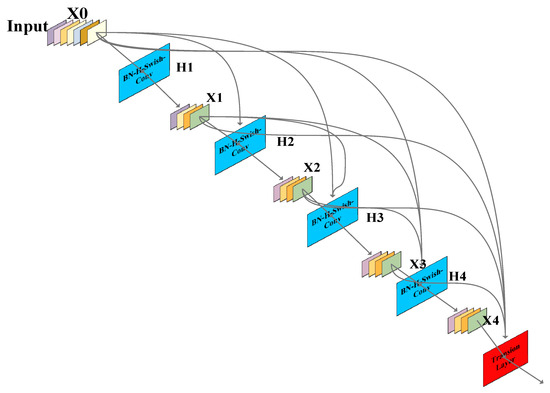
Figure 1.
Structure of a dense block in YOLOC.
Compared to the widely used residual structure, which is also used in the backbone network of YOLOv4, DenseNet utilizes a dense connection strategy that aggressively links all the layers together. In DenseNet, each layer is connected to all previous layers in the channel dimension and serves as the input for the next layer. The number of connections in DenseNet is calculated as follows:
where is the total number of connections, and is the number of network layers.
It is precisely due to the dense connection structure in the dense block of the YOLOC backbone network, which directly connects feature maps from different layers, that feature reuse is enabled and the utilization efficiency of features is improved. This results in more abundant features extracted with the detection model for vehicle images, which facilitates better recognition. Meanwhile, this dense connection structure also strengthens the flow of gradients, with more skip connections making the gradient easier to propagate forward. Additionally, this structure can obtain more features with fewer parameters, greatly reducing the number of parameters in the detection model.
3.3. The Lightweight Neck and Head with DSC
To further reduce the computational expense and parameter quantity of the vehicle detector, depth-wise separable convolution (DSC) [14] is used in the neck and head of YOLOC. Specifically, the 3 × 3 ordinary convolution of the neck and head is modified to DSC. DSC requires lower computational costs than ordinary convolution. Standard convolution applies the same convolution kernel to all channels of the image for the convolution operation, and different convolution kernels are used to extract different features. The convolution kernel of standard convolution is designed for all channels of the input image. Therefore, every time an input image adds a channel, a convolution kernel needs to be added. Finally, standard convolution merges all the inputs to obtain a new output. The calculation expression of the output of a standard convolution is shown in Equation (9), and the computational cost consumption expression is outlined in Equation (10). Depth-wise separable convolution divides standard convolution into 3 × 3 depth-wise convolution and 1 × 1 point-wise convolution, which is shown in Figure 2. Firstly, 3 × 3 depth-wise convolution extracts different features using different convolution kernels on various channels of the image. However, this operation only extracts one aspect of the feature for a specific channel. Therefore, 1 × 1 point-wise convolution is added on this basis to extract different features from the feature map and produce the same output feature map as standard convolution. These two operations greatly reduce the computational expense and parameter quantity. The calculation expression of the output of a depth-wise separable convolution is illustrated in Equation (11), and the computational cost consumption expression is outlined in Equation (12). The expression for the ratio of computational expense between DSC and standard convolution is shown in Equation (13). This equation indicates that the parameter count of DSC is much less than that of ordinary convolution. Therefore, using DSC instead of standard convolution outside the backbone can effectively reduce the parameter count of the detection model. Figure 3 illustrates the structure of DSC in YOLOC. The structures of the neck and head lightweighted via depth-wise separable convolution are shown in Figure 4 and Figure 5, respectively.
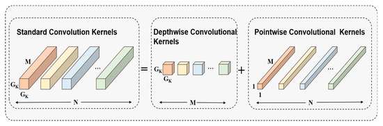
Figure 2.
Equivalent schematic diagram of standard convolution and depth-wise separable convolution (including depth-wise convolution and point-wise convolution).
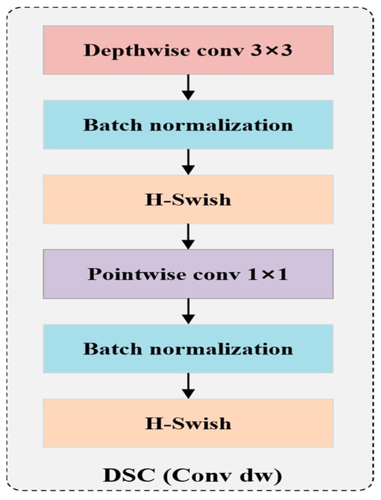
Figure 3.
The structure of DSC in YOLOC.
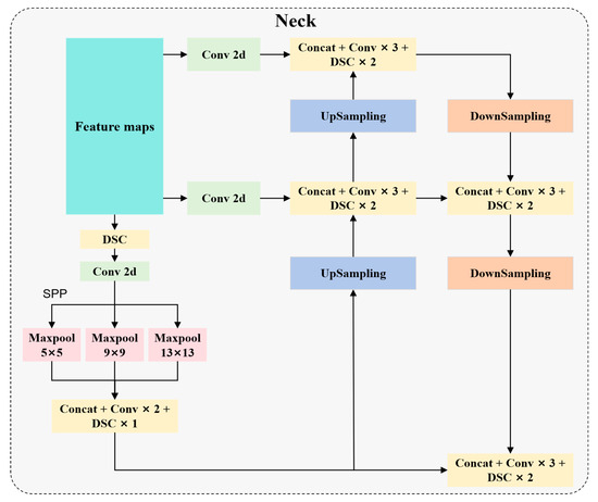
Figure 4.
Structure of lightweighted neck with DSC of YOLOC.
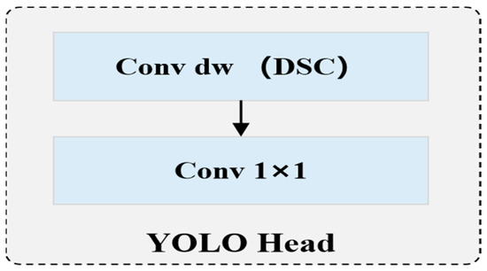
Figure 5.
Structure of a YOLO head lightweighted with DSC of YOLOC.
Here, and represent the outputs of standard convolution and depth-wise separable convolution, respectively. and represent their convolution kernels. denotes the features to be convolved. and are the positions of the pixels. represents the m-th channel of the convolution kernel, and denotes the number of convolution kernels. represents the output of standard convolution. and represent the computational costs of standard convolution and DSC, respectively. denotes the width and height of the input feature map. represents the spatial dimension of the convolution kernel. denotes the number of input channels, and represents the number of output channels.
3.4. The H-Swish Activation Function
Choosing an appropriate activation function to improve the identification precision and performance of the vehicle detector is an important aspect of developing such models. In the backbone network of YOLOv4, Leaky ReLU, as the main activation function, is used outside of the backbone network, and its calculation expression is shown in Equation (14). The Leaky ReLU activation function solves the problem of neuronal death caused by the ReLU function, and its slight positive incline in the negative domain enables backpropagation to be performed on negative input values. Yet, the utilization of the Leaky ReLU activation function across various intervals could result in incongruous outcomes, rendering it incapable of offering dependable forecasts of relationships for both negative and positive input values. Therefore, in the proposed YOLOC model for urban construction-related vehicle detection, the H-Swish function was used as the main activation function, and its calculation expression is shown in Equation (15). The function graphs of Leaky ReLU and H-Swish are shown in Figure 6.
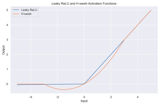
Figure 6.
Function graph of H-Swish and Leaky ReLU.
From the calculation expression and function graph of the H-Swish activation function, it is apparent that this activation function possesses the following advantages:
- Similar to the ReLU function, it has no upper limit. This characteristic is required for any activation function. It can prevent gradient saturation, which results in a significant decline in the speed of training. Therefore, this feature ensures that it does not suffer from gradient saturation problems and can accelerate the training of detection models.
- It has a lower bound (the left half-axis of x gradually tends to 0). This can produce stronger regularization effects and effectively prevent overfitting.
- Non-monotonic function: this characteristic preserves minor negative values, leading to a stable gradient flow in the network. Most commonly used activation functions cannot maintain negative values, making most neurons unable to be updated.
- It is continuous and differentiable everywhere, making it easier to train.
- The H-Swish activation function is a differentiable function with robust generalization capability and efficient optimization ability, which can significantly enhance the recognition accuracy of neural networks.
In summary, the unique non-monotonicity of H-Swish enhances the model’s detection precision for urban construction activities related to vehicles. Due to the absence of an upper limit but the presence of a lower limit, it can effectively address the saturation issue of input neurons and enhance the regularization impact of the model [49]. Furthermore, it offers computational efficiency advantages over the Swish function, which facilitates the training process. Additionally, it considerably minimizes the memory accesses required for the detection model.
3.5. The Proposed Vehicle Detector, YOLOC
Figure 7 depicts the architecture of the suggested vehicle detector, YOLOC. Compared with YOLOv4, YOLOC exhibits significant advantages in both detection accuracy and parameter quantity. Feature extraction of the input vehicle images is performed using DenseNet121, which has dense connections instead of the original CSPDarkNet53 as the backbone network. In DenseNet, the fully connected layer used for classification is removed, but other parts are retained, including the 3 × 3 convolutional layer of its head, pooling layers, and the dense block structure, to maintain consistency in the network. The improved YOLOv4 algorithm YOLOC uses DenseNet121 as the feature extraction network, which not only alleviates gradient vanishing but also strengthens the feature extraction and transfer of urban construction-related vehicles in the network, more effectively reusing features, greatly enhancing feature utilization efficiency, and improving the recognition precision of the detection model for vehicles. Therefore, only the number of feature layer channels is changed in the detection network, while the size of the feature layers in the network remains the same as before. Additionally, due to the dense connection mechanism of DenseNet, the number of model parameters is greatly reduced. Furthermore, in addition to improving the backbone feature extraction network of YOLOC, the 3 × 3 standard convolution of the neck and head was also optimized by modifying it to DSC, further reducing the parameter quantity and computational expense of the detection model. In addition, the H-Swish activation function is utilized as the primary activation function of the detector. Compared with the Leaky ReLU activation function mainly used in YOLOv4, H-Swish can not only perform better non-linear feature extraction but also has better generalization ability and result optimization ability, enabling the model to better recognize vehicles and further enhance the identification precision of the detector for vehicles. These experiments showed that after these modifications, the model can effectively solve the problems of low recognition precision and high computational cost in the current vehicle methods, and its performance in vehicle detection exceeds that of other SOTA detectors.
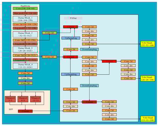
Figure 7.
Network structure of the proposed detection model, YOLOC.
Furthermore, the loss function of YOLOC primarily consists of the subsequent components: object position loss function (), classification loss function (), and confidence loss function (). The loss function is calculated as follows:
The object position loss function () is computed using the following formula:
where represents the prediction box, is the real box, is the Euclidean distance between the center point of the prediction box and the center point of the real box, represents the diagonal distance of the smallest closed rectangular area that can contain both the prediction box and the real box, denotes the intersection ratio of the prediction box and the ground truth, and represent the width and height of the real boundary box, respectively, and and denote the width and height of the predicted boundary box, respectively.
The computational formula for the classification loss function () is as follows:
where is the number of grids to divide the image, represents whether the th grid contains the target in the th prediction box (if it contains it, its value is 1; otherwise, it is 0), represents the probability of the target object category in the prediction box, is the probability of the target object category in the real box, is the object category, and is the total number of target object categories.
The computational formula for the confidence loss function () is as follows:
where is the total number of target object categories, represents the error weight parameter, is whether the th grid contains the target object in the th prediction box (if it does not, its value is 1; otherwise it is 0), is the confidence of the ground truth, and represents the confidence of the predicted box.
4. Dataset
In Section 4, the methods of data collection and the cameras used are introduced. Further, the process of data pre-processing will also be described.
4.1. Data Collection
The proposed dataset for urban construction-related vehicle activities was captured using a high-definition camera mounted on a tall tower. The specific model of the high-definition camera used was iDS-2DY9437IX-A/SP. The collected images of vehicles related to urban construction activities were captured in various scenes within the city. This includes common vehicles in building scenes, as well as vehicles captured in traffic and residential environments. Table 2 displays the parameters of the high-definition camera used for capturing vehicle images. The images in this dataset were captured under natural conditions, encompassing various scenes, weather conditions, occlusions, and overlaps, with a size of 1080 × 1920 pixels. The dataset consists of 8425 images, containing 13 classes of vehicles related to urban construction activities. According to the functionality and appearance of vehicle images in this dataset, they are divided into 13 categories, such as big truck, small truck, earth vehicle (medium truck) used for transportation, and digger for digging.
Table 2.
Parameter values of our camera.
4.2. Data Pre-Processing
All collected vehicle images were initially cropped to a size of 416 × 416 pixels. This not only alleviates the problem of data imbalance (to a certain extent) in the dataset but also further expands the quantity of image data, thereby enlarging the scale of the dataset. Then, using the open-source image annotation tool LableImg, all vehicle images were manually annotated to obtain the class and location information of the vehicles in the captured images. Finally, all annotated vehicle images, along with their corresponding annotation files, were organized in the format of the Pascal VOC dataset for training detection models. Table 3 illustrates the names and descriptions of each class of vehicles in the dataset. Figure 8 shows a number of sample images of vehicles in the dataset. The quantity and proportion of images for each class in the dataset are shown in Figure 9 and Figure 10, respectively. The number of sample images for each category in this dataset exceeds 200, which ensures the effectiveness and availability of the dataset. It can be seen that the numbers of sample images for boxcar, digger, and big truck in this dataset were the highest. The numbers of sample images for tractor, fuel tank, and crane closed in the dataset were the lowest. The number of image samples in the first three categories was approximately 800 more than that in the last three categories. There is a category imbalance issue with the proposed dataset.
Table 3.
Category and description of urban construction activity-related vehicles.
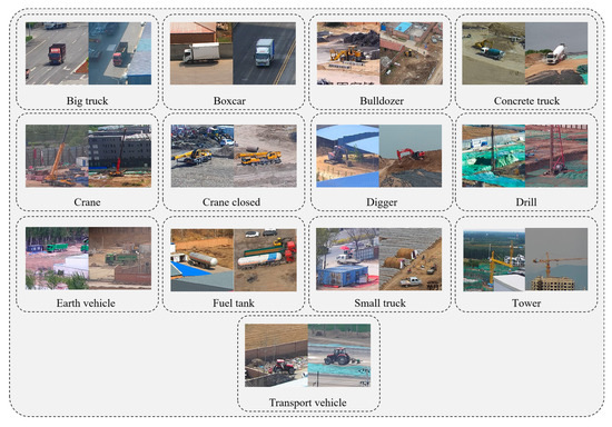
Figure 8.
Samples images of vehicles in the proposed dataset.
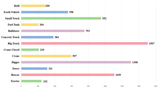
Figure 9.
The number of images for each category of vehicles in the proposed dataset.
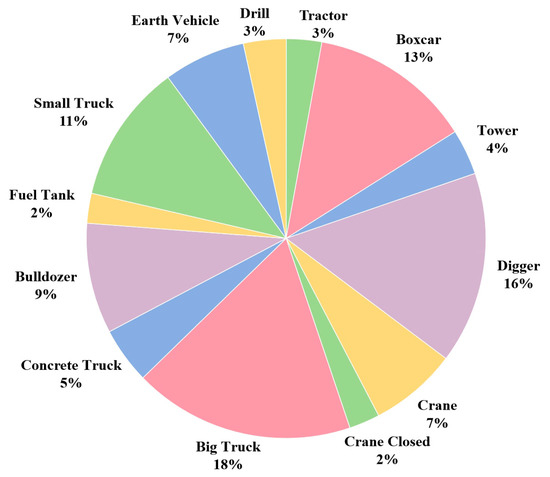
Figure 10.
The ratio of the number of vehicle images for each category in the proposed dataset.
5. Experiment
5.1. Experimental Setting
All experiments in this study were performed on a GPU server with a graphics card, NVIDIA GeForce GTX Titan X, 12 GB of memory, and Ubuntu 18.04 as the operating system. The server configuration details are provided in Table 4. The proposed detection model, YOLOC, was trained using both pre-training and fine-tuning approaches. Initially, the detector was trained on the Pascal VOC dataset; then, it was fine-tuned using the proposed vehicle dataset. The proposed vehicle dataset was split into a training set, a validation set, and a test set, with 6824, 758, and 843 images, respectively. The YOLOC detection model was trained for 100 epochs, utilizing the Adam optimizer. For the first 50 epochs, the backbone network (Densenet121) was frozen and only trained the non-backbone parts of the model. In the subsequent 50 epochs, the entire model was trained with the unfrozen backbone network. The learning rate was set to 0.001 for the first 50 epochs and 0.0001 for the last 50 epochs, with the batch size being 16 for the first 50 epochs and 8 for the remaining 50 epochs. YOLOv4 and YOLOC adopted the same batch size, learning rate, and learning method, and they also trained with the pre-trained models. YOLOv4 and YOLOC had the same hyperparameter settings, and the training, validation, and testing sets they used were also the same. They conducted all the experiments on the same server. In the comparative experiment and the ablation experiment, the experimental settings of the two were the same.
Table 4.
Configuration information of the GPU server.
5.2. Evaluation Metrics
To evaluate the efficacy of the proposed vehicle detection model, this work chose to use commonly employed metrics in the field of object detection. These metrics are mAP, AP, precision, recall, and F1 score, and their respective calculation formulas are listed below:
where represents precision, represents recall, represents F1 score, and represents the number of vehicles correctly identified as vehicles with the algorithm. It represents the detector’s correct detection of actual vehicles. is the number of non-vehicles incorrectly identified as vehicles using the proposed detector. It indicates the detector falsely labeling non-existent vehicles as vehicles. is the number of vehicles incorrectly identified as non-vehicles with the algorithm. Vehicle detection involves two sub-tasks: classification and localization. Vehicles not only need to be correctly classified but also must be accurately localized to be detected.
6. Results and Analysis
6.1. Comparison with YOLOv4
To evaluate the performance of the proposed vehicle detection model, it was compared with YOLOv4. All experiments were conducted using the proposed vehicle dataset. The experimental results are shown in Table 5. The values of precision, recall, and F1 score for YOLOv4 were 90.62%, 90.13%, and 90.19%, respectively, while for YOLOC, they were 95.85%, 94.89%, and 95.24%, respectively. The mAP values for YOLOv4 and YOLOC were 92.92% and 96.95%, respectively. Compared to the original YOLOv4, YOLOC achieved higher precision, recall, and F1 score values, with increases of 5.23%, 4.76%, and 5.05%, respectively. In terms of the most important evaluation metric, mAP, YOLOC outperformed YOLOv4 by 4.03%. In the proposed dataset of 13 categories of urban construction activity-related vehicles, YOLOC demonstrated higher AP values than YOLOv4 for 12 vehicle classes. However, in the detection of transport vehicles alone, the AP value was 80.42%, which was 2.24% lower than that of YOLOv4. These findings indicate the effectiveness of the proposed improvement method, significantly enhancing the recognition accuracy of YOLOv4 for vehicles. Sample detection result images are shown in Figure 11. As shown in Figure 11, both YOLOC and YOLOv4 accurately recognize and locate vehicle images under various scenarios, enabling high-precision detection of vehicle images. The sample images with failed detection of YOLOC are shown in Figure 12. Several cars and trucks were not detected. This may be due to the appearance captured by vehicles from different perspectives being different. Moreover, there are few sample images from this angle in the dataset, resulting in missed detections. Although there were a few missed detections in the dataset, we will address this issue in future work.
Table 5.
Results of a comparative experiment with YOLOv4.
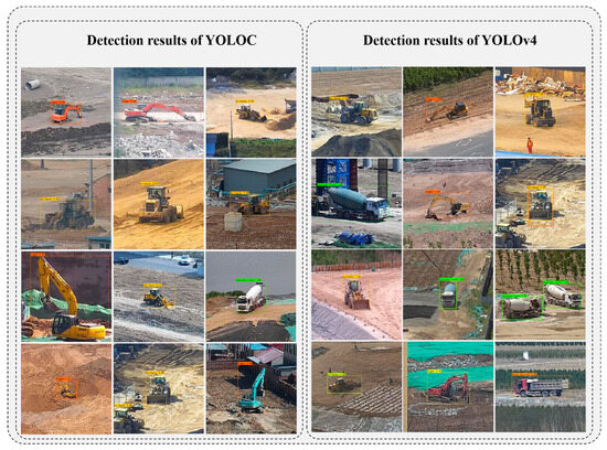
Figure 11.
Sample vehicle images of detection results of YOLOC.
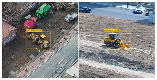
Figure 12.
Several examples of images with missed detection.
6.2. Comparison with other Detectors
In addition, this work also compared the proposed vehicle detector, YOLOC, with several popular and state-of-the-art (SOTA) object detectors. As illustrated in Table 6, different detection performance metrics of YOLOC, such as mAP, precision, recall, and F1 score, were compared with existing SOTA object detection models (e.g., Faster R-CNN, RetinaNet, EfficientDet, SSD, YOLOv3, YOLOv4, YOLOX, and YOLOv5), all of which were trained on the proposed vehicle dataset alongside YOLOC. The training, validation, and testing sets for the experiments remained unchanged.
Table 6.
Results of comparative experiments with other state-of-the-art detectors.
As shown in Table 6, the mAP values of RetinaNet and YOLOv8 were over 95.00%. The mAP values of SSD, Faster R-CNN, YOLOv3, YOLOv4, YOLOv7, and DETR were between 92.00% and 95.00%. The mAP values of the YOLOv5 series were between 91.00% and 94.00%. The mAP values of the EfficientDet series were between 89.00% and 92.00%. The mAP value of YOLOX was 84.64%, which is the lowest. The proposed detector, YOLOC, achieved the highest mAP value of 96.95%. RetinaNet closely followed, with an mAP of 95.98%. The mAP values of these two models were quite similar, while the mAP values of the other detectors were significantly lower. The state-of-the-art object detection model, YOLOv8, had a lower mAP and F1 score than YOLOC, with mAP and F1 score values of 93.90% and 92.94%, respectively. Additionally, the proposed YOLOC model achieved an F1 score of 95.24%, surpassing other popular SOTA detectors (e.g., YOLOv5, YOLOX, and YOLOv8). On the evaluation metric of F1 score, YOLOC was 95.24%, which is the highest of these detectors. Further, the precision and recall values of YOLOC were 95.85% and 94.89%, respectively. The values of the other detectors were lower than those for YOLOC.
Moreover, the proposed vehicle detector, YOLOC, has a parameter count of 16.08 MB and a computational load of 26.09GFLOPs. Compared to YOLOv4, it has reduced its parameter count by 74.88% and decreased its computational load by 56.52%. Furthermore, the parameter count and computational cost of the proposed YOLOC model were significantly lower than for other popular SOTA object detectors, such as YOLOv3, SSD, RetinaNet, YOLOv7, and Faster R-CNN. It requires a lower memory load and computational resources, making it more suitable for mobile and smart devices. Therefore, the proposed detection model can accurately detect vehicles related to urban construction activities, providing assistance in traffic management and urban planning to promote urban development.
6.3. Ablation Study
Table 7 illustrates the results obtained using YOLOv4 as the baseline model on the proposed vehicle dataset, along with the improved detection results. YD represents the utilization of DenseNet121 as the backbone network to enhance the utilization efficiency of vehicle features, thereby significantly improving the accuracy of vehicle recognition while reducing computational costs and parameters. YM represents the modification of the 3 × 3 standard convolution outside the backbone network to DSC to further reduce the parameters of the detection model. YA denotes the use of the H-Swish activation function instead of LeakyReLU to enhance the detection accuracy of the model. YDM represents the use of DenseNet121 as the backbone network and DSC outside the backbone network. YDA represents that DenseNet121 is used as the backbone network and H-Swish is used instead of the Leaky ReLU activation function. YMA represents the use of DSC outside the backbone network and using H-Swish instead of the Leaky ReLU activation function. YOLOC is the proposed detector, integrating all the improved methods.
Table 7.
Results of the ablation experiment.
The baseline model YOLOv4 achieved an mAP value of 92.92%. After modifying the original backbone network CSPDarkNet53 to DenseNet121, the mAP value improved to 95.88%, representing a 2.96% increase compared to the unimproved version. When only incorporating DSC into the detection model structure, the mAP value reached 93.59%, showing a 0.67% improvement. By using the H-Swish activation function outside the backbone network, the mAP value obtained was 94.77%, which is a 1.85% improvement over YOLOv4. By replacing CSPDarkNet53 with DenseNet121 for feature extraction and further incorporating the DSC modification, the mAP value reached 96.06%. Compared to YOLOv4, this is a 3.14% improvement. When using DenseNet121 for feature extraction and employing the H-Swish activation function, the mAP value of the detector reached 96.56%, indicating a 3.64% improvement over YOLOv4. With the optimization of both DSC and H-Swish, the mAP value reached 95.50%, a 1.87% improvement over YOLOv4. When all the optimization methods were applied to the baseline YOLOv4 model, the mAP value reached 96.95%, reflecting a 4.03% improvement over the original YOLOv4. Furthermore, the proposed detector, YOLOC, achieved an F1 score value that was 5.05% higher than YOLOv4, indicating significant improvements in detection accuracy and avoiding false positives. This is crucial for practical applications of vehicle detection models, as a higher F1 score means that the model can accurately identify and locate vehicles, providing more reliable results.
7. Conclusions
This paper proposed a high-precision and lightweight detector for construction-related vehicles and constructed a vehicle dataset. The proposed dataset comprises 8425 vehicle images related to 13 categories of construction activities. Compared to previous vehicle detection algorithms, YOLOC achieved higher detection accuracy with lower computational costs. The backbone of YOLOC employed DenseNet121 with the dense connection mechanism to enhance feature transmission and reuse. Further, DSC was introduced into its neck and head to further reduce parameters and computational costs, optimize the model structure, and decrease computational and memory consumption. H-Swish, as the primary activation function, enhanced the model’s ability to learn non-linear features in vehicle images, improving the optimization and generalization capabilities of the model and further increasing detection accuracy. Compared to existing SOTA detection models, YOLOC achieved the highest detection accuracy on the proposed construction activity-related vehicle dataset. A series of experimental results showed that this detector is very suitable for construction activity-related vehicles, with the characteristics of low computational cost, low storage load, and high detection accuracy.
In the future, we will address the issue of the poor detection performance of YOLOC under low-light and occlusion situations, and we will introduce diffusion models and multimodality generation technologies to address the issue of category imbalance in datasets. In addition, we will also introduce techniques such as model compression, knowledge distillation, and multimodality to improve detection accuracy and reduce the parameters and computational costs of the detection model.
Author Contributions
W.L.: Conceptualization, Data curation, Formal analysis, Methodology, Investigation, Writing—original draft. S.Z.: Conceptualization, Data curation, Formal analysis, Resources, Supervision, Writing—review and editing. L.Z.: Methodology, Project administration, Supervision, Writing—review and editing. N.L.: Funding acquisition, Supervision, Writing—review and editing. M.X.: Funding acquisition, Supervision, Writing—review and editing. All authors have read and agreed to the published version of the manuscript.
Funding
This work was supported, in part, by the National Natural Science Foundation of China (nos. 62177034 and 61972046).
Data Availability Statement
The data that support the findings of this study are available from the corresponding author upon reasonable request.
Conflicts of Interest
The research was conducted in the absence of any commercial or financial relationships that could be construed as a potential conflict of interest.
Correction Statement
This article has been republished with a minor correction to resolve spelling and grammatical errors. This change does not affect the scientific content of the article.
References
- Cheon, M.; Lee, W.; Yoon, C.; Park, M. Vision-based vehicle detection and tracking for intelligent transportation systems. IEEE Trans. Ind. Inform. 2014, 10, 1397–1406. [Google Scholar]
- Zaman, F.T.; Kurt, G.K. Vehicle detection and tracking in urban traffic surveillance: A comprehensive survey. IET Intell. Transp. Syst. 2016, 10, 619–629. [Google Scholar]
- Nguyen, T.; Chen, Y.; Kankanhalli, M.S.; Nguyen, T.Q. Vehicle detection in urban traffic scenes: A survey. IEEE Trans. Circuits Syst. Video Technol. 2016, 26, 1019–1034. [Google Scholar]
- Li, X.; Xie, Y.; Wang, J.; Li, T. Vehicle detection in urban traffic scenes: A comprehensive survey. ACM Comput. Surv. 2016, 48, 1–31. [Google Scholar] [CrossRef]
- Wang, C.; Wang, H.; Li, B. Vehicle detection using partial shape features. IEEE Trans. Intell. Transp. Syst. 2013, 14, 230–240. [Google Scholar]
- Li, X.Q.; Song, L.K.; Choy, Y.S.; Bai, G.C. Multivariate ensembles-based hierarchical linkage strategy for system reliability evaluation of aeroengine cooling blades. Aerosp. Sci. Technol. 2023, 138, 108325. [Google Scholar] [CrossRef]
- Srikar, M.; Malathi, K. An Improved Moving Object Detection in a Wide Area Environment using Image Classification and Recognition by Comparing You Only Look Once (YOLO) Algorithm over Deformable Part Models (DPM) Algorithm. J. Pharm. Negat. Results 2022, 13, 1701–1707. [Google Scholar]
- Yar, H.; Khan, Z.A.; Ullah, F.U.M.; Ullah, W.; Baik, S.W. A modified YOLOv5 architecture for efficient fire detection in smart cities. Expert Syst. Appl. 2023, 231, 120465. [Google Scholar] [CrossRef]
- Dilshad, N.; Ullah, A.; Kim, J.; Seo, J. LocateUAV: Unmanned aerial vehicle location estimation via contextual analysis in an IoT environment. IEEE Internet Things J. 2022, 10, 4021–4033. [Google Scholar] [CrossRef]
- Park, J.; Baek, J.; Kim, J.; You, K.; Kim, K. Deep Learning-Based Algal Detection Model Development Considering Field Application. Water 2022, 14, 1275. [Google Scholar] [CrossRef]
- Zhou, Z.H.; Zhang, M.L. A brief introduction to weakly supervised learning. Natl. Sci. Rev. 2017, 4, 697–712. [Google Scholar] [CrossRef]
- Bochkovskiy, A.; Wang, C.Y.; Liao, H.Y.M. Yolov4: Optimal speed and accuracy of object detection. arXiv 2020, arXiv:2004.10934. [Google Scholar]
- Huang, G.; Liu, Z.; Van Der Maaten, L.; Weinberger, K.Q. Densely connected convolutional networks. In Proceedings of the IEEE Conference on Computer Vision and Pattern Recognition, Honolulu, HI, USA, 21–26 July 2017; pp. 4700–4708. [Google Scholar]
- Howard, A.G.; Zhu, M.; Chen, B.; Kalenichenko, D.; Wang, W.; Weyand, T.; Adam, H. Mobilenets: Efficient convolutional neural networks for mobile vision applications. arXiv 2017, arXiv:1704.04861. [Google Scholar] [CrossRef]
- Howard, A.; Sandler, M.; Chu, G.; Chen, L.C.; Chen, B.; Tan, M.; Adam, H. Searching for mobilenetv3. In Proceedings of the IEEE/CVF International Conference on Computer Vision; 2019; pp. 1314–1324. [Google Scholar] [CrossRef]
- Horn, B.K.P.; Schunck, B.G. Determining optical flow. Artif. Intell. 1981, 17, 185–203. [Google Scholar] [CrossRef]
- Barnich, O.; Van Droogenbroeck, M. ViBe: A universal background subtraction algorithm for video sequences. IEEE Trans. Image Process. 2011, 20, 1709–1724. [Google Scholar] [CrossRef]
- Rin, V.; Nuthong, C. Front moving vehicle detection and tracking with Kalman filter. In Proceedings of the 2019 IEEE 4th International Conference on Computer and Communication Systems (ICCCS), Singapore, 23–25 February 2019; pp. 304–310. [Google Scholar]
- Sun, W.; Sun, M.; Zhang, X.; Li, M. Moving vehicle detection and tracking based on optical flow method and immune particle filter under complex transportation environments. Complexity 2020, 2020, 3805320. [Google Scholar] [CrossRef]
- Ge, D.Y.; Yao, X.F.; Xiang, W.J.; Chen, Y.P. Vehicle detection and tracking based on video image processing in intelligent transportation system. Neural Comput. Appl. 2023, 35, 2197–2209. [Google Scholar] [CrossRef]
- Wan, S.; Ding, S.; Chen, C. Edge computing enabled video segmentation for real-time traffic monitoring in internet of vehicles. Pattern Recognit. 2022, 121, 108146. [Google Scholar] [CrossRef]
- El Jaafari, I.; El Ansari, M.; Koutti, L.; Ellahyani, A.; Charfi, S. A novel approach for on-road vehicle detection and tracking. Int. J. Adv. Comput. Sci. Appl. 2016, 7. [Google Scholar]
- Wei, Y.; Tian, Q.; Guo, J.; Huang, W.; Cao, J. Multi-vehicle detection algorithm through combining Harr and HOG features. Math. Comput. Simul. 2019, 155, 130–145. [Google Scholar] [CrossRef]
- Şentaş, A.; Tashiev, İ.; Küçükayvaz, F.; Kul, S.; Eken, S.; Sayar, A.; Becerikli, Y. Performance evaluation of support vector machine and convolutional neural network algorithms in real-time vehicle type and color classification. Evol. Intell. 2020, 13, 83–91. [Google Scholar] [CrossRef]
- Goerick, C.; Noll, D.; Werner, M. Artificial neural networks in real-time car detection and tracking applications. Pattern Recognit. Lett. 1996, 17, 335–343. [Google Scholar] [CrossRef]
- Jabri, S.; Saidallah, M.; El Alaoui, A.E.B.; El Fergougui, A. Moving vehicle detection using Haar-like, LBP and a machine learning Adaboost algorithm. In Proceedings of the 2018 IEEE International Conference on Image Processing, Applications and Systems (IPAS), Sophia Antipolis, France, 12–14 December 2018; pp. 121–124. [Google Scholar]
- Kowsari, T.; Beauchemin, S.S.; Cho, J. Real-time vehicle detection and tracking using stereo vision and multi-view AdaBoost. In Proceedings of the 2011 14th International IEEE Conference on Intelligent Transportation Systems (ITSC), Washington, DC, USA, 5–7 October 2011; pp. 1255–1260. [Google Scholar]
- Wang, L.W.; Yang, X.F.; Siu, W.C. Learning approach with random forests on vehicle detection. In Proceedings of the 2018 IEEE 23rd International Conference on Digital Signal Processing (DSP), Shanghai, China, 19–21 November 2018; pp. 1–5. [Google Scholar]
- Halin, A.A.; Sharef, N.M.; Jantan, A.H.; Abdullah, L.N. License plate localization using a Naïve Bayes classifier. In Proceedings of the 2013 IEEE International Conference on Signal and Image Processing Applications, Melaka, Malaysia, 8–10 October 2013; pp. 20–24. [Google Scholar]
- Duarte, M.F.; Hu, Y.H. Vehicle classification in distributed sensor networks. J. Parallel Distrib. Comput. 2004, 64, 826–838. [Google Scholar] [CrossRef]
- Bhatt, C.; Kumar, I.; Vijayakumar, V.; Singh, K.U.; Kumar, A. The state of the art of deep learning models in medical science and their challenges. Multimed. Syst. 2021, 27, 599–613. [Google Scholar] [CrossRef]
- Yao, S.; Guan, R.; Huang, X.; Li, Z.; Sha, X.; Yue, Y.; Lim, E.G.; Seo, H.; Man, K.L.; Zhu, X.; et al. 2d car detection in radar data with pointnets. In Proceedings of the 2019 IEEE Intelligent Transportation Systems Conference (ITSC), Auckland, New Zealand, 27–30 October 2019; pp. 61–66. [Google Scholar]
- Najafabadi, M.M.; Villanustre, F.; Khoshgoftaar, T.M.; Seliya, N.; Wald, R.; Muharemagic, E. Deep learning applications and challenges in big data analytics. J. Big Data 2015, 2, 1. [Google Scholar] [CrossRef]
- Abdar, M.; Pourpanah, F.; Hussain, S.; Rezazadegan, D.; Liu, L.; Ghavamzadeh, M.; Fieguth, P.; Cao, X.; Khosravi, A.; Acharya, U.R.; et al. A review of uncertainty quantification in deep learning: Techniques, applications and challenges. Inf. Fusion 2021, 76, 243–297. [Google Scholar] [CrossRef]
- Valappil, N.K.; Memon, Q.A. CNN-SVM based vehicle detection for UAV platform. Int. J. Hybrid Intell. Syst. 2021, 17, 59–70. [Google Scholar] [CrossRef]
- Chen, R.; Li, X.; Li, S. A lightweight CNN model for refining moving vehicle detection from satellite videos. IEEE Access 2020, 8, 221897–221917. [Google Scholar] [CrossRef]
- Xiao, Y.; Tian, Z.; Yu, J.; Zhang, Y.; Liu, S.; Du, S.; Lan, X. A review of object detection based on deep learning. Multimed. Tools Appl. 2020, 79, 23729–23791. [Google Scholar] [CrossRef]
- Sang, J.; Wu, Z.; Guo, P.; Hu, H.; Xiang, H.; Zhang, Q.; Cai, B. An improved YOLOv2 for vehicle detection. Sensors 2018, 18, 4272. [Google Scholar] [CrossRef]
- Song, H.; Liang, H.; Li, H.; Dai, Z.; Yun, X. Vision-based vehicle detection and counting system using deep learning in highway scenes. Eur. Transp. Res. Rev. 2019, 11, 51. [Google Scholar] [CrossRef]
- Murugan, V.; Vijaykumar, V.R.; Nidhila, A. A deep learning RCNN approach for vehicle recognition in traffic surveillance system. In Proceedings of the 2019 International Conference on Communication and Signal Processing (ICCSP), Chennai, India, 4–6 April 2019; pp. 0157–0160. [Google Scholar]
- Shi, F.; Zhang, T.; Zhang, T. Orientation-aware vehicle detection in aerial images via an anchor-free object detection approach. IEEE Trans. Geosci. Remote Sens. 2020, 59, 5221–5233. [Google Scholar] [CrossRef]
- Zhang, X.; Zhu, X. Vehicle detection in the aerial infrared images via an improved Yolov3 network. In Proceedings of the 2019 IEEE 4th International Conference on Signal and Image Processing (ICSIP), Wuxi, China, 19–21 July 2019; pp. 372–376. [Google Scholar]
- Mahto, P.; Garg, P.; Seth, P.; Panda, J. Refining yolov4 for vehicle detection. Int. J. Adv. Res. Eng. Technol. IJARET 2020, 11. [Google Scholar]
- Chen, Z.; Cao, L.; Wang, Q. Yolov5-based vehicle detection method for high-resolution UAV images. Mob. Inf. Syst. 2022, 2022, 1828848. [Google Scholar] [CrossRef]
- Liu, W.; Anguelov, D.; Erhan, D.; Szegedy, C.; Reed, S.; Fu, C.Y.; Berg, A.C. Ssd: Single shot multibox detector. In Proceedings of the Computer Vision–ECCV 2016: 14th European Conference, Amsterdam, The Netherlands, 11–14 October 2016; Proceedings, Part I 14. Springer International Publishing: Berlin/Heidelberg, Germany, 2016; pp. 21–37. [Google Scholar]
- Arora, N.; Kumar, Y.; Karkra, R.; Kumar, M. Automatic vehicle detection system in different environment conditions using fast R-CNN. Multimed. Tools Appl. 2022, 81, 18715–18735. [Google Scholar] [CrossRef]
- Kashevnik, A.; Ali, A. 3D Vehicle Detection and Segmentation Based on EfficientNetB3 and CenterNet Residual Blocks. Sensors 2022, 22, 7990. [Google Scholar] [CrossRef] [PubMed]
- Bisio, I.; Haleem, H.; Garibotto, C.; Lavagetto, F.; Sciarrone, A. Performance evaluation and analysis of drone-based vehicle detection techniques from deep learning perspective. IEEE Internet Things J. 2021, 9, 10920–10935. [Google Scholar] [CrossRef]
- He, K.; Zhang, X.; Ren, S.; Sun, J. Spatial pyramid pooling in deep convolutional networks for visual recognition. In European Conference on Computer Vision; Springer: Berlin/Heidelberg, Germany, 2014; pp. 346–361. [Google Scholar]
- Liu, S.; Qi, L.; Qin, H.; Shi, J.; Jia, J. Path aggregation network for instance segmentation. In Proceedings of the IEEE Conference on Computer Vision and Pattern Recognition; 2018; pp. 8759–8768. [Google Scholar] [CrossRef]
Disclaimer/Publisher’s Note: The statements, opinions and data contained in all publications are solely those of the individual author(s) and contributor(s) and not of MDPI and/or the editor(s). MDPI and/or the editor(s) disclaim responsibility for any injury to people or property resulting from any ideas, methods, instructions or products referred to in the content. |
© 2023 by the authors. Licensee MDPI, Basel, Switzerland. This article is an open access article distributed under the terms and conditions of the Creative Commons Attribution (CC BY) license (https://creativecommons.org/licenses/by/4.0/).