A Review of Homography Estimation: Advances and Challenges

Abstract

Images captured from different viewpoints or devices have often exhibited significant geometric and photometric differences due to factors such as environmental variations, camera technology differences, and shooting conditions’ instability. To address this problem, homography estimation has attracted much attention as a method to describe the geometric projection relationship between images. Researchers have proposed numerous homography estimation methods for single-source and multimodal images in the past decades. However, the comprehensive review and analysis of homography estimation methods, from feature-based to deep learning-based, is still lacking. Therefore, we provide a comprehensive overview of research advances in homography estimation methods. First, we provide a detailed introduction to homography estimation’s core principles and matrix representations. Then, we review homography estimation methods for single-source and multimodal images, from feature-based to deep learning-based methods. Specifically, we analyze traditional and learning-based methods for feature-based homography estimation methods in detail. For deep learning-based homography estimation methods, we explore supervised, unsupervised, and other methods in-depth. Subsequently, we specifically review several metrics used to evaluate these methods. After that, we analyze the relevant applications of homography estimation and show the broad application prospects of this technique. Finally, we discuss current challenges and future research directions, providing a reference for computer vision researchers and engineers.

1. Introduction

Today, images captured from various viewpoints or equipment, including remote sensing satellites, can display considerable geometric and photometric variances caused by factors like fluctuating environmental conditions, dissimilarities in camera technology, and unstable shooting scenarios. This difference makes combining or comparing these images difficult, affecting many applications such as augmented reality [1,2,3], object recognition [4,5], and panoramic stitching [6,7,8]. To solve this problem, researchers have employed various image processing techniques such as image registration [9,10], color correction [11,12], and homography estimation [13]. Among these techniques, homography estimation has received considerable attention for its ability to describe the geometric projection relationship between images.

Existing geometric projection transformation models mainly include projection transformations, rigid body transformations, and affine transformations. Rigid and affine transformations are only suitable for certain deformations and small perspective changes. In contrast, the projective transformation is a more complex transformation model capable of handling a broader range of viewpoint changes and perspective distortions. Homography estimation focuses on determining a projective transformation between two images [14]. With this transformation, we can effectively understand and compensate for the geometric differences between the images, leading to better image registration. The central of this method is the homography matrix, which can process geometric changes such as rotation, translation, scaling, and projection [15,16]. With decades of research, numerous homography estimation methods have been proposed for various applications, such as image registration [17], image fusion [18,19], and object tracking [20].

Early research in homography estimation concentrated on single-source images from the same sensor or modality. Differences between these images were often caused by camera movement or rotation. So, early methods [21,22,23] used local features of the image, such as corner points and edges, for estimation. These traditional methods become inadequate when faced with large geometric variations, occlusions, or nonlinear photometric changes. With the rise of deep learning techniques, researchers are beginning to apply their powerful representation learning capabilities to capture critical information and structure from images more effectively.

With time, technology and application requirements have changed. Researchers have realized that only processing single-source images is not enough. In practical scenarios, such as medical image fusion [24] or multimodal image registration [25], the images to be processed are often from different sensors or modalities. This not only presents the challenge of geometric variations but also introduces photometric differences resulting from different sensors or modalities. Therefore, cross-sensor or cross-modality homography estimation has become an important and challenging research direction, leading researchers to turn to multimodal image homography estimation.

The overall structure of this survey is shown in Figure 1. Section 2 describes its central principle and matrix representations in detail. In Section 3, we then discuss advances in homography estimation methods, especially for single-source and multimodal images. To enable a comprehensive evaluation of these methods, Section 4 provides a series of evaluation metrics of homography estimation methods for researchers’ reference. Meanwhile, in Section 5, we discuss the applications of homography in various fields. Then, Section 6 explores current research challenges and considers possible future research directions. Finally, in Section 7, we summarise this paper’s primary points and homography’s development process.

2. Homography Transformation of Images

In this section, we first introduce the homography principle and show a simple procedure for calculating homography matrices. Secondly, we show two representations of the homography matrix.

2.1. Homography Principle

Homography transformation of images is usually defined as the projection mapping relationship between images of the same planar object taken from different positions by two lens distortion-free cameras [26]. Specifically, it describes the transformation relationship from one plane to another, as shown in Figure 2.

The homography matrix is often used to represent the homographic transformation relationship between two images. The homography matrix $H$ is defined as follows:

$$H=\left[\begin{array}{ccc}{h}_{11}& h_{12}& h_{13}\\ h_{21}& h_{22}& h_{23}\\ h_{31}& h_{32}& h_{33}\end{array}\right]$$

(1)

where $[h_{11}, h_{12}, h_{21},h_{22}]$, $[h_{13}, h_{23}]$ and $[h_{31}, h_{32}]$ represent the affine transformation, the translation transformation, and the perspective transformation between images, respectively. Additionally, the coordinate transformation relationship between the corresponding points of the two images can be expressed as:

$$\left[\begin{array}{c}{x}^{\prime }\\ y^{\prime }\\ 1\end{array}\right]=H\left[\begin{array}{c}x\\ y\\ 1\end{array}\right]=\left[\begin{array}{ccc}{h}_{11}& h_{12}& h_{13}\\ h_{21}& h_{22}& h_{23}\\ h_{31}& h_{32}& h_{33}\end{array}\right]\left[\begin{array}{c}x\\ y\\ 1\end{array}\right]$$

(2)

where $(x, y, 1)$ represents the homogeneous coordinates of a feature point in the first image; $(x^{\prime }, y^{\prime }, 1)$ denotes the homogeneous coordinates of the corresponding point in the other image; and $H$ stands for the homography matrix. Expand Equation (2), we can get:

$$\begin{array}{c}{x}^{\prime }=h_{11}x+h_{12}y+h_{13}\\ y^{\prime }=h_{21}x+h_{22}y+h_{23}\\ 1=h_{31}x+h_{32}y+h_{33}\end{array}$$

(3)

Then, put the third equation into the first two equations, and we can obtain the following:

$$\begin{array}{c}{x}^{\prime }=\frac{x^{\prime }}{1}=\frac{h_{11}x+h_{12}y+h_{13}}{h_{31}x+h_{32}y+h_{33}}\\ y^{\prime }=\frac{y^{\prime }}{1}=\frac{h_{21}x+h_{22}y+h_{23}}{h_{31}x+h_{32}y+h_{33}}\end{array}$$

(4)

Further, by multiplying the denominator to the left, we can transform it into:

$$\begin{array}{c}\left(h_{31}x+h_{32}y+h_{33}\right)x^{\prime }=h_{11}x+h_{12}y+h_{13}\\ \left(h_{31}x+h_{32}y+h_{33}\right)y^{\prime }=h_{21}x+h_{22}y+h_{23}\end{array}$$

(5)

Moving the left-hand side of the equation over to the right-hand side, we can transform this into:

$$\begin{array}{c}0=(h_{11}x+h_{12}y+h_{13})-\left(h_{31}{x}^{\prime }x+h_{32}{x}^{\prime }y+h_{33}{x}^{\prime }\right)\\ 0=(h_{21}x+h_{22}y+h_{23})-\left(h_{31}{y}^{\prime }x+h_{32}{y}^{\prime }y+h_{33}{y}^{\prime }\right)\end{array}$$

(6)

We are rewriting Equation (6) using matrix notation as $Ah=0$ results in the expression for Equation (7).

$$0=Ah=\left[\begin{array}{ccccccccc}x& y& 1& 0& 0& 0& -x^{\prime }x& -x^{\prime }y& -x^{\prime }\\ 0& 0& 0& x& y& 1& -y^{\prime }x& -y{\prime }^y& -y^{\prime }\end{array}\right]\left[\begin{array}{c}{h}_{11}\\ h_{12}\\ h_{13}\\ h_{21}\\ h_{22}\\ h_{23}\\ h_{31}\\ h_{32}\\ h_{33}\end{array}\right]$$

(7)

where $h={[h_{11}, h_{12}, h_{13}, h_{21}, h_{22}, h_{23}, h_{31}, h_{32}, h_{33}]}^T$, is a nine-dimensional column vector.

The homography matrix $H$ is a $3\times 3$ homogeneous matrix. Its final element, $h_{33}$, is normalized to 1 so that $H$ has only 8 degrees of freedom. To solve the homography matrix, we need corresponding coordinate points. Two linear equations can be derived from each pair of matched coordinate points. Therefore, we need at least four pairs of corresponding points to compute the homography matrix between two images [27]. In practice, we usually use more than four pairs of corresponding points because of the coordinate errors caused by noise. Finally, Direct Linear Transformation (DLT) [28] and Singular Value Decomposition (SVD) [29] are used to obtain the homography matrix.

2.2. Homography Matrix Representations

In homography estimation methods, the representation of the homography matrix can be divided into two representations: the 4-point parameterization and the homography flow. In this section, we will introduce them separately.

2.2.1. 4-Point Parameterization

The homography matrix has eight degrees of freedom, so finding four pairs of corresponding matches between two images solves the homography matrix. In deep learning-based homography estimation methods, it is not appropriate to use the parameter expansion of the $3\times 3$ form of the homography matrix as the regression value predicted by the deep learning method. This is because the parameters within the homography matrix are mixed with different meanings. For instance, the rotation and scaling of the affine transform is denoted by $[h_{11},h_{12},h_{21},h_{22}]$, and the translation is denoted by $[h_{13},h_{33}]$. The rotation terms usually have smaller values than the translation terms, and balancing both terms in an optimization problem is challenging. Additionally, it is difficult to enforce non-singular constraints on the predicted homography matrix $H$ [30]. Therefore, a four-point parameterized form is commonly used in deep learning-based homography estimation methods to tackle these concerns [31]. The 4-point parameterized homography matrix $H_{4points}$ can be expressed as follows:

$$H_{4points}=\left[\begin{array}{cc}\Delta x_1& \Delta y_1\\ \Delta x_2& \Delta y_2\\ \Delta x_3& \Delta y_3\\ \Delta x_4& \Delta y_4\end{array}\right]$$

(8)

where $(x_i, y_i)$ and $(x_i^{\prime }, y_i^{\prime })$ denote the corresponding points between the two images; $\Delta x_i={ x}_i^{\prime }-x_i$ and $\Delta y_i=y_i^{\prime }-y_i$ represent the offsets of the horizontal and vertical coordinates of the corresponding points, respectively. The four-point parameterized form of the homography matrix $H_{4points}$ and the $3\times 3$ form of the homography matrix $H$ are equivalent. However, the four-point parameterized form of the matrix is more conducive to network training and convergence [32]. Finally, it is converted into a homography matrix by the DLT algorithm. This process is shown in Figure 3.

2.2.2. Homography Flow

The homography flow presents a novel approach to solving homography matrices [33]. It is characterized as a specialized form of optical flow, with dimensions of $H\times W\times 2$, and subject to homography constraints. The central concept entails producing eight stream bases by modifying the entries of one homography matrix at a time, thereby yielding eight homography matrices. Each matrix is subsequently converted into a stream map in relation to the image coordinates. This yields eight homography stream bases and reconstructs homography streams $H_{ab}$ by learning to combine weights in the space spanned by said stream bases. As it is constrained by homography, the flow that responds alone falls into an 8-dimensional subspace within the $2HW-D$ space of the optical flow. Therefore, it can be represented by the eight positive alternating current bases that span the subspace, as demonstrated in:

$$\begin{array}{c}\exists {\{h}_i\} s.t. h_{ab}=\sum _i{w}_i{h}_i (i=1, 2, \dots , 8)\\ where h_i\in {\mathbb{R}}^{2HW}, h_i^T{h}_j=0\end{array}$$

(9)

where $h_{ab}$ is the tiled version of $H_{ab}$ and $\left\{w_i\right\}$ are the coefficients of the flow basis. To obtain an orthogonal flow basis, eight homography matrices are generated by modifying each entry $h_i$ of the unit homography matrix, except that the entry located at position $(3, 3)$ is always normalized to 1. Then, given the image coordinates, the homography matrices can be converted to homography flow maps by transforming the image coordinates and subtracting their original positions. Then, the eight homography streams are normalized by their maximum stream amplitude and then $QR$ decomposed. It can be described as:

$$M=Q\cdot R \left(M, Q\in {\mathbb{R}}^{2HW\times 8}, R\in {\mathbb{R}}^{8\times 8}\right)$$

(10)

where each column of the matrix $M$ represents a tiling-normalized homography flow $H_i$, following the method described above. Via $QR$ decomposition, each column of $Q$ becomes orthogonal, forming flow bases that span the homography subspace, denoted as $Q=\{h_1, h_2, \dots , h_8\}$. This means that each flow base is associated with a tangent space at the origin of the homography group. The final predicted homography flow is then achieved by accurately predicting the weights $\left\{w_i\right\}$ of each of the eight flow bases. Figure 4 illustrates the flow represented by the block diagram.

3. Homography Estimation Methods

We present a summary and classification of these studies and propose a structural block diagram illustrated in Figure 5. Numerous studies have advanced methods for estimating image homography. Homography estimation is classified into two categories: single-source image homography estimation methods and multi-source image homography estimation methods based on image sources. Each category is further subdivided. We will comprehensively review each method in detail.

3.1. Single-Source Image Homography Estimation Methods

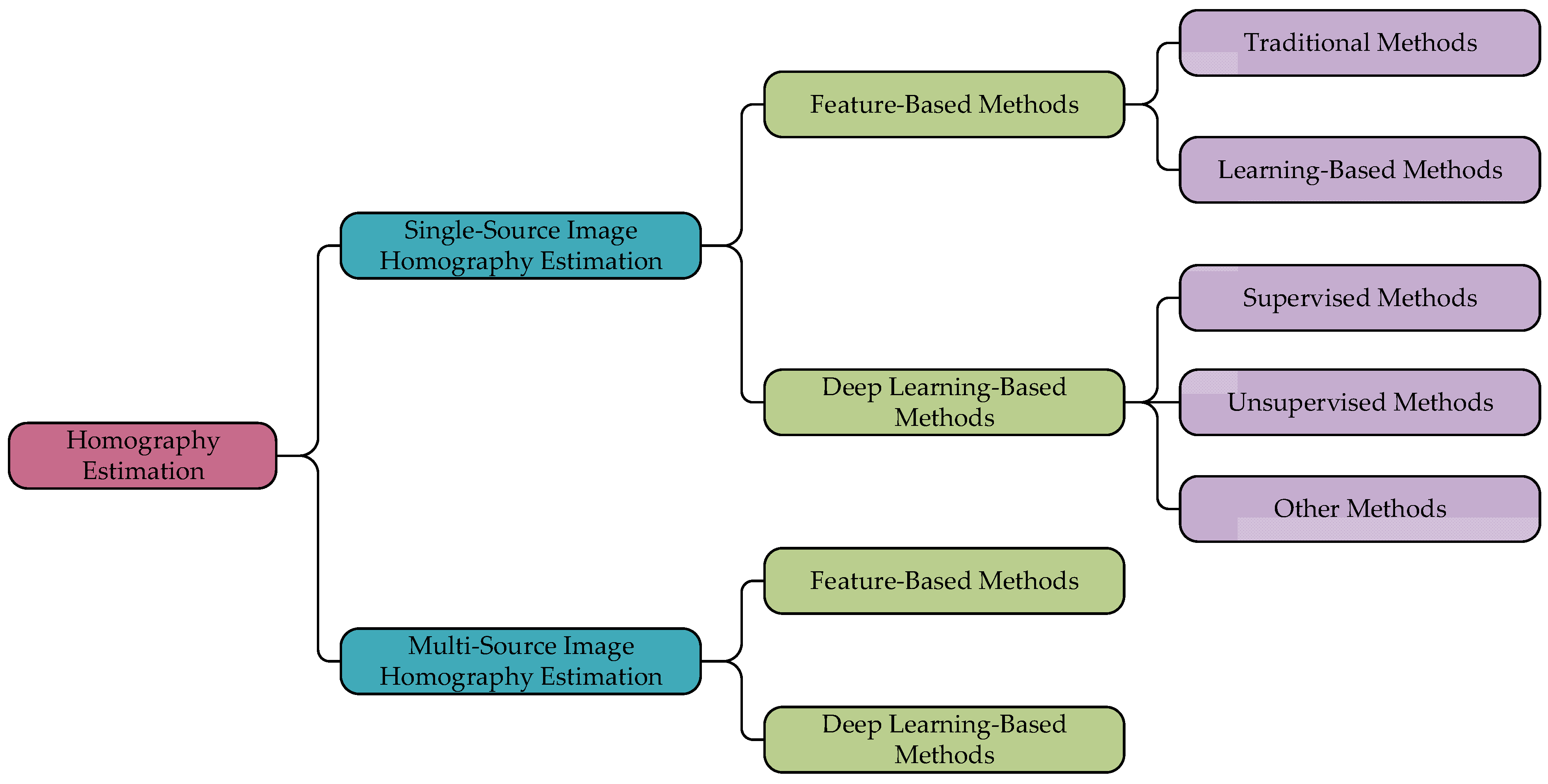
Single-source images are usually acquired by the same equipment from different viewpoints or at different times. These images often show significant geometric variations due to small camera positions or viewing angle changes. To accurately align these images, homography estimation becomes a powerful tool. At this stage, homography estimation algorithms for single-source images can be classified into feature-based and deep learning-based methods.

3.1.1. Feature-Based Methods

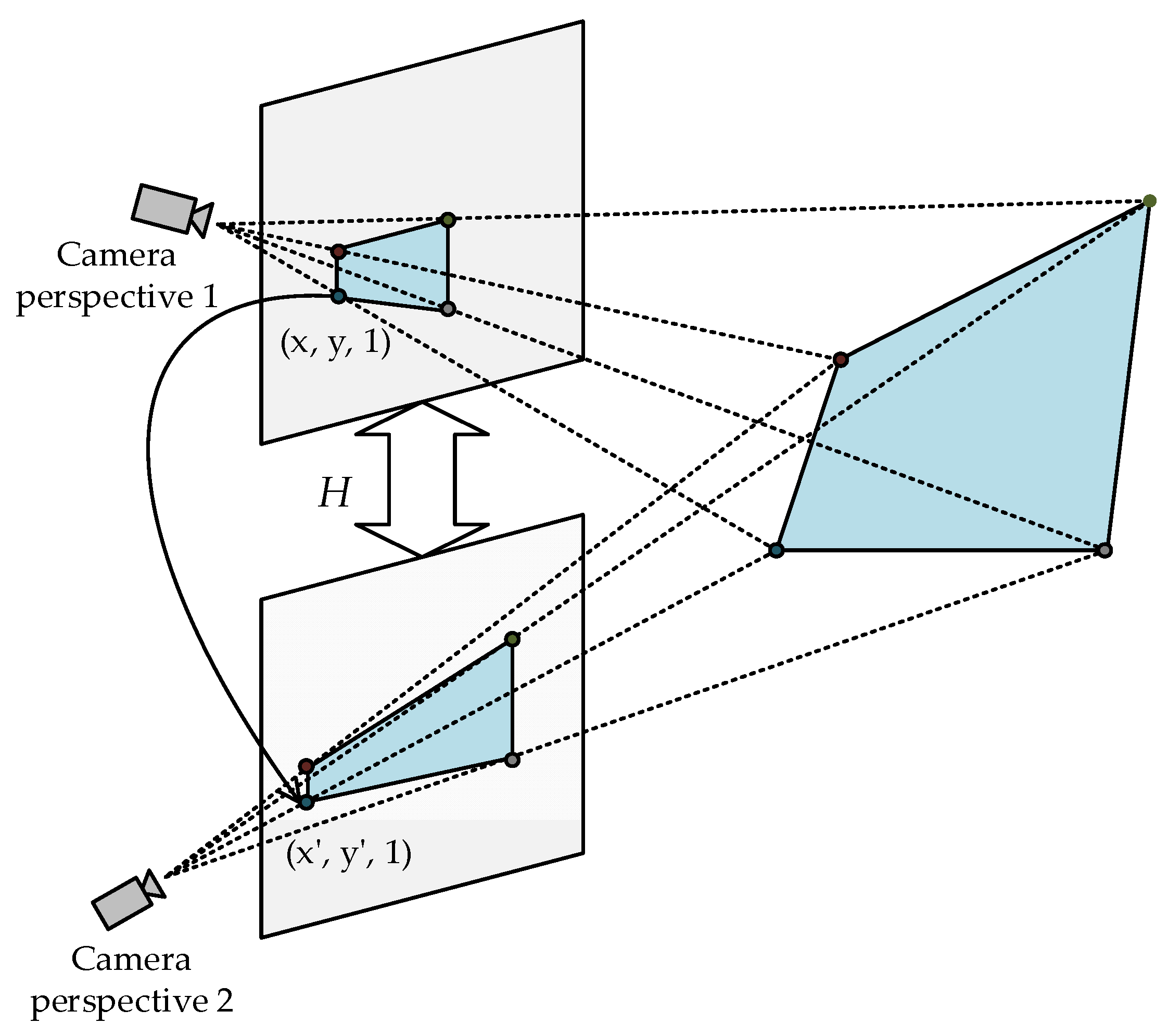
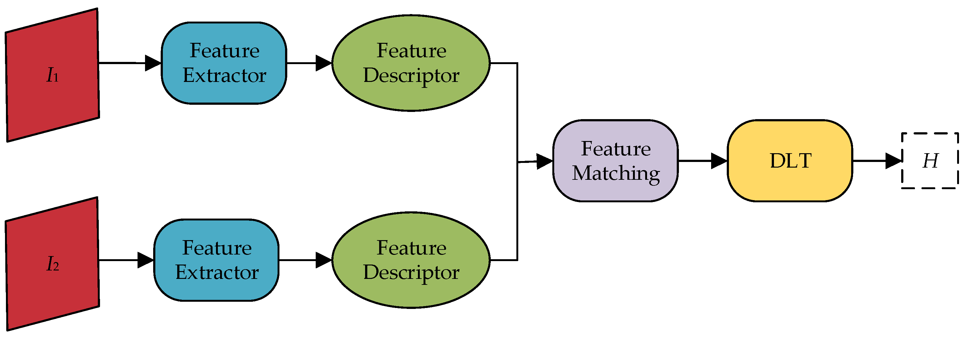
The feature-based homography estimation method first detects the feature points in the image by a feature extraction algorithm and computes the similarity metric for matching. Then, utilizing the mapping relationship of the matched feature points, the parameters of the homography matrix are solved [34]. This procedure is illustrated in Figure 6. Feature-based methods can be further divided into two categories: traditional methods and learning-based methods.

Traditional Methods. Traditional methods are divided into three main steps: feature detection, feature matching, and homography matrix solving. Firstly, feature extraction algorithms are used to detect feature points in the image and to extract descriptors around these feature points, which are generally represented as vectors. Common methods for extracting features include Scale Invariant Feature Transform (SIFT) [21], Speeded Up Robust Features (SURF) [22], Oriented FAST and Rotated BRIEF (ORB) [23], etc. Similarity measures like the Hamming or Euclidean distance are calculated to provide a criterion for matching feature points. Finally, to improve the estimation’s robustness, e.g., RANSAC or other robust estimation algorithms are usually used to find a consistent subset from these matches and thus estimate the homography matrix.

In recent years, feature point extraction algorithms have received attention and improvement from many researchers. In 2012, Chum et al. [35] proposed a novel homography matrix estimation method. This method is based on the correspondence between two or more local elliptic features and is estimated using a first-order Taylor expansion. Notable, only one homography model was generated for each pair of elliptic features. This design not only reduces computational costs but also enhances accuracy. In 2014, Liu et al. [36] proposed BB-Homography, a joint binary feature and bipartite graph matching algorithm for homography estimation. First, BB-Homography employs bipartite Graph Matching (GM) to enhance the matching results of binary descriptors and ascertain the correlation between preliminary keypoint correspondences and homography estimation. Next, GM is iteratively executed to refine the results to obtain more accurate homography estimates. Yan et al. [37] proposed a Homography Estimation method based on Appearance Similarity and Keypoint correspondence (HEASK), combining the keypoint correspondence and appearance similarity models. In the keypoint correspondence model, the Laplace distribution replaces the Gaussian distribution to represent the distribution of inlier location error. In the appearance similarity model, the Enhanced Correlation Coefficient (ECC) is used to describe image similarity. The combination of these two models makes the results of the homography estimation more robust.

In 2016, Zhao et al. [38] proposed a feature-based homography estimation method to enhance estimation accuracy and better handle positioning errors. The method introduces the compensation, representation, and weighting methods for localization error based on existing methods to alleviate the problem of degradation of estimation accuracy and robustness caused by localization error. Specifically, it uses High-accurate localized features for SIFT (HALF-SIFT) to compensate for localization errors caused by feature extraction and the covariance matrix to describe localization errors caused by image noise. However, the running time of the method is long. In 2019, Barath et al. [39] proposed a geometric interpretation of the angles and scales provided by orientation and scale-variant feature detectors such as SIFT. They introduced two new generic constraints for scales and rotations and designed a new solver capable of estimating the single homography matrix from at least two correspondences. Suárez et al. [40] proposed Boosted Efficient Binary Local Image Descriptor (BEBLID) in 2020. This method is similar to SIFT in accuracy but better in computational efficiency than ORB.

After the SIFT algorithm was proposed, some traditional methods considered tradeoffs in the balance between speed and accuracy. One Improving approach is HALF-SIFT, which aims to improve accuracy. Other algorithms, such as ORB and BEBLID, are developed to balance computation time and accuracy. Therefore, algorithms such as SIFT or HALF-SIFT are better for images with complex scene changes. For cases requiring a higher response speed, it is preferable to use algorithms such as SURF and BEBLID.

Furthermore, besides refining the feature extraction algorithms, some scholars focus on improving the RANSAC outlier suppression algorithm. Examples include FT-RANSAC [41], MAGSAC++ [42]. In 2023, Rodríguez et al. [43] proposed several modifications to the RANSAC algorithm. The method combines affine approximation and an inverse approach to improve the homography estimation between pairs of images. This inverse approach defines estimation robustness and enables adaptive thresholding to differentiate outliers, improving the success rate of image pair recognition.

Notable, most traditional homography estimation algorithms are based on calculating the mapping relationship between feature points to solve the homography matrix, but some scholars hold a different view. They believe that line feature-based homography estimation methods outperform feature point-based methods in terms of performance, mainly because line features are usually more noise-resistant than point features in detection. In 2008, Dubrofsky et al. [44] proposed an extended normalized direct linear transformation algorithm. The approach integrates the correspondence of line features into the computation of the homography matrix by introducing line normalization equations that are compatible with point normalization. However, Zeng et al. [45] pointed out that line-based homography estimation can be highly unstable when the image line passes through or near the origin. To tackle this issue, they proposed a novel line normalization method. The approach first performs a normalization transformation on the corresponding line segments of the two sets of images to make their distribution in the images more uniform. Subsequently, the DLT algorithm is employed on this new set of line correspondences to solve the homography matrix. In 2016, Huang et al. [46] proposed a homography estimation method for ellipses using a common self-polar triangle of two ellipses. The method obtained the correspondence of four lines using the quadratic curves and the self-polar triangles, which provides sufficient computational conditions for homography estimation.

Based on this, some researchers began using the correspondences of point and line features to solve the homography [47,48]. In other words, by effectively using all available point and line correspondences, the accuracy of homography estimation can be significantly improved under different measurement conditions. This brings a new direction for further research. However, whether based on point features or line features, the performance of traditional homography estimation methods is still not stable enough in highly noisy or non-texture images. In addition,

Table 1. Single-source image homography estimation algorithm based on traditional methods. The table lists the year of publication, core ideas, advantages, and limitations of each method.

Method			Refer.	Year	Core Idea	Advantages	Limitations
Traditional Methods	Point Feature	SIFT	[21]	2004	A technique for extracting distinct, invariant features from images.	The descriptors are invariant to image scale and rotation and are robust in most scenes.	There is a substantial computational workload.
		SURF	[22]	2006	A new detector and descriptor for interest points are introduced, with invariance to scale and rotation.	It surpasses preceding methods in terms of repeatability, uniqueness, and robustness.	Runs slower than ORB and is less accurate than SIFT.
		ORB	[23]	2011	Presented aa rapid binary descriptor founded on BRIEF.	Rotation invariant and resistant to noise.	Trade accuracy for speed, less accurate than SIFT.
		Homography estimation from correspondences of local elliptical features	[35]	2012	Estimating homography from the correspondence of two or more local elliptic features.	Develop models with comparable or greater accuracy than at the time, at lower computational cost.	The quadratic constraint arising from the rotation is ignored in the estimation.
		BB-Homography	[36]	2014	A novel approach that merges fast binary descriptor matching and bipartite graph for homography estimation.	Attains high homography estimation accuracy while maintaining high computational speed.	Dose not solve the problem of 3D rigid and non-rigid pose estimation yet.
		HEASK	[37]	2014	Combine the probability models of keypoint correspondences and appearance similarity in a Maximum Likelihood framework.	Consistently achieves accurate homography estimation under different transformation degrees and different inlier ratios.	Because of ECC calculations, HEASK methods are more time-consuming than others.
		Accurate and robust feature-based homography estimation using HALF-SIFT and feature localization error weighting	[38]	2016	Compensating and representing localization error with the HALF-SIFT method and covariance matrix.	More accurate and robust under varying noise levels and inlier ratios.	Requires a longer run time.
		Homography from two orientation-and scale-covariant features	[39]	2019	Proposed the geometric interpretation of feature detectors regarding angle and scale.	Robust calculators require fewer iterations and yield stable numerical results.	The performance could be impacted by severe variability conditions.
		BEBLID	[40]	2020	A binary image descriptor efficiently learned.	Produces improved local descriptors and resolves the asymmetry issue in matching and retrieval.	Accuracy still slightly lower than SIFT.
		Robust homography estimation from local affine maps	[43]	2023	Applies affine approximations and a-contrario procedures to improve homography estimation.	Enhancing the likelihood of accurately identifying image pairs within difficult matching databases.	The number of internal iterations of the RANSAC algorithm does not decrease.
	Line Feature	Combining line and point correspondences for homography estimation	[44]	2008	The derivation of a line normalization equation compatible with point normalization.	Will produce more accurate results when there are more point correspondences than line correspondences.	The correspondence between point and line could be non-existent or inconsistent.
		A new normalized method on line-based homography estimation	[45]	2008	A new normalized method designed for line-based homography estimation.	Removing the risk cases and increasing the accuracy and robustness.	Normalization may introduce noise and impose limitations on non-linear transformations.
		Homography estimation from the common self-polar triangle of separate ellipses	[46]	2016	Homography estimation using four-line correspondences obtained from common self-polar triangles.	No requirements on the physical information of the patterns and the camera and no ambiguity on the solution.	Does not apply to other distributions of two coplanar ellipses or circles yet.

provides a comprehensive analysis of homography estimates from traditional models.

Learning-Based Methods. Learning-based methods for homography estimation use neural networks to replace the feature extraction or feature matching in traditional algorithms and then use traditional methods to estimate the homography transformation parameters at other steps. Both learning-based and traditional methods involve feature detection, feature matching, and homography matrix solving. The main difference is that traditional methods usually rely on hand-designed feature extractors to detect and match local features, and learning methods use convolutional neural networks to detect or match features.

In 2016, Yi et al. [49] proposed the Learned Invariant Feature Transform (LIFT) algorithm, which combines local features for detection and description. It does so by integrating three standard pipeline components into a differentiable network and training end-to-end using backpropagation. In 2018, DeTone et al. [50] presented the Self-Supervised Interest Point Detection and Description (SSIPD) algorithm, known as the SuperPoint algorithm. The algorithm can simultaneously compute pixel-level interest point locations and corresponding descriptors in forward passes by running a fully convolutional model on a full-size image. They further propose a multi-scale, multi-homography method to improve the reproducibility of interest point detection and enable cross-domain adaptation (e.g., from synthetic to real). Notable, the SuperPoint algorithm can identify a wider range of points of interest compared to both the original pre-adapted depth model and other traditional corner detectors. In 2019, Tian et al. [51] proposed the Similarity Regularization for Local Descriptor Learning (SOS-Net) algorithm, which incorporates second-order similarity into local descriptor learning to achieve more precise outcomes. Zhang et al. [52] proposed the Order-Aware Networks (OANs) for probabilistic outlier detection and relative pose regression encoded in the underlying matrix. OANs comprise three hierarchical operations. Firstly, the correspondences of unordered inputs are clustered to capture the local context of sparse correspondences by learning soft assignment matrices. These clusters have a canonical order and are independent of input alignment. Second, these clusters relate to each other spatially to form the global context of the correspondences. Finally, the context-encoded clusters are restored to their original size using an upsampling operator.

As feature information extracted by neural networks gradually becomes complex, researchers find that the traditional feature-matching methods have limitations. Thus, they began to use neural networks to replace the feature-matching algorithms [53,54,55]. In 2020, Sarlin et al. [56] proposed SuperGlue, a local feature-matching network based on Graph Neural Networks (GNN). SuperGlue uses a flexible attention-based context aggregation mechanism to jointly reason about the underlying 3D scene and feature assignments over the complete graph. Moreover, it matches local features via the joint identification of correspondences and rejection of non-matchable points. In 2022, Shi et al. [57] proposed a Cluster-based Coarse-to-Fine Graph Neural Network (ClusterGNN). Compared to SuperGlue, ClusterGNN integrates a progressive clustering module to decrease redundant connections in the whole graph computation, thus reducing the misclassification of images and improving feature-matching accuracy. Wang et al. [58] proposed a hierarchical feature extraction and matching transformer called MatchFormer. MatchFormer uses a lightweight decoder similar to Feature Pyramid Network (FPN) to fuse multi-scale features and integrates self-attention and cross-attention to perform feature extraction and feature similarity learning to achieve the best feature matching. These methods show that neural networks have equally powerful capabilities for feature matching.

The feature estimation method’s accuracy has been improved by replacing the feature extraction or matching parts of the traditional method with neural networks. However, since the other processes and outlier suppression still use traditional methods, they still have some shortcomings when faced with challenging image scenarios. Nonetheless, the learning-based methods also bring new insights that influence the development of deep learning-based homography estimation methods. In addition,

Table 2. Single-source image homography estimation algorithm based on traditional methods. The table includes every approach’s publication year, core ideas, advantages, and limitations.

Method		Refer.	Year	Core Idea	Advantages	Limitations
Learning Based Methods	LIFT	[42]	2016	Combines the pipelines for local feature detection and description into a single differentiable network.	Implementing hard negative mining techniques across the image to obtain more precise descriptors.	Requires supervision from classical Structure-from-Motion (SfM) system.
	Super Point	[43]	2018	A self-supervised framework for training interest point detectors and descriptors.	Capable of detecting a more diverse range of interest points compared to other detectors.	Model performance requires improvement in semantic segmentation and object detection and poor results in outdoor scenes.
	SOS-Net	[44]	2019	Incorporate second-order similarity regularization into training.	Achieve outstanding results in several standard benchmark tests across various tasks.	The localized patch dataset used in paper does not guarantee sufficient intra-class samples to accurately estimate the parameters.
	OANs	[45]	2019	Propose an Order-Aware Network and regress the relative pose encoded by the essential matrix.	The accuracy of the two-view geometry and correspondences is improved compared to the state of the art.	Re-train all models on the same data. If training a larger model, this model drops on unknown scenes.
	SuperGlue	[56]	2020	Matches two groups of local features by collectively finding correspondences whilst rejecting non-matchable points.	Enabling highly accurate relative pose estimation on extreme wide-baseline indoor and outdoor image pairs.	Complete graph representation results in wasteful attention-based message passing and suffers from computational and memory complexity.
	Clustergnn	[57]	2022	An attentional GNN architecture that operates on clusters to learn the feature-matching task.	Significant decrease in both runtime and memory usage in the detection of dense objects.	Unable to extract repeated keypoints when dealing with image pairs with large variations in appearance.
	MatchFormer	[58]	2022	Interleave self-attention for the extraction of features and cross-attention for matching features.	A multi-win solution in efficiency, robustness, and precision.	Work entirely in the 2D image domain, ignoring the underlying 3D geometry of the scene.

presents a detailed examination of learning-based homography estimation for single-source images.

3.1.2. Deep Learning-Based Methods

With the development of deep learning techniques, it has achieved excellent results in the field of computer vision, especially in tasks such as image classification, target detection, and semantic segmentation. Notable, more and more scholars have begun to apply deep learning to the research of homography estimation, and significant progress has been achieved. Compared to learning-based methods, deep learning-based methods transform the traditional multi-step feature extraction and matching process into a unified, trainable framework that novelty understands and handles complex image correspondences. This technique dramatically improves the efficiency and quality of feature extraction and opens new ways to improve matching accuracy and robustness.

These deep learning-based homography estimation methods can be mainly classified into two categories: supervised and unsupervised. They usually adopt two forms of homography matrix representation: 4-point parameterization and homography flow. Specifically, the 4-point parameterized form is commonly used in both supervised and unsupervised methods, while the homography flow form is mainly used in unsupervised methods.

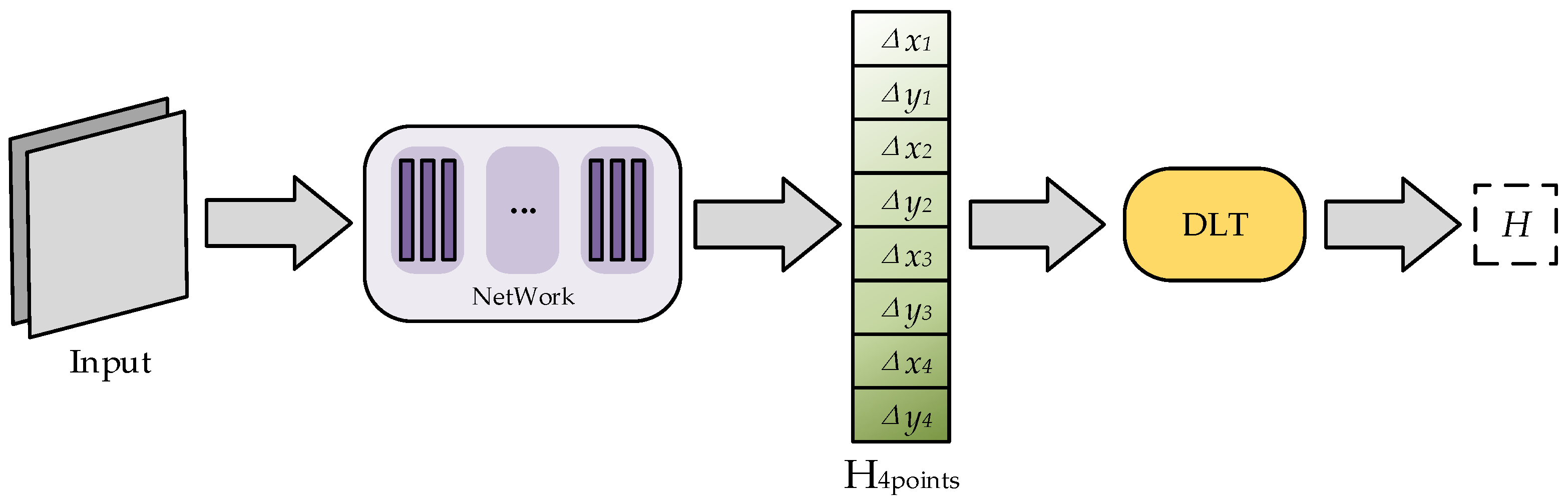
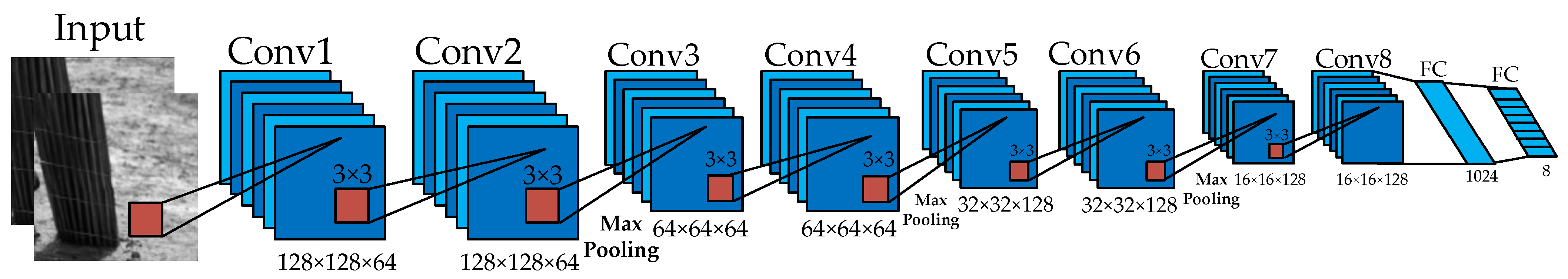
Supervised Methods. Supervised homography estimation methods primarily utilize synthetic examples with ground-truth labels to train the network. In 2016, DeTone et al. [31] pioneered the introduction of deep learning into the field of homography estimation, propounding a 4-point parametric representation of the homography matrix for network training and convergence. Figure 7 shows their network structure. This research utilizes Convolutional Neural Networks (CNNs) to automatically learn and predict geometric transformations between images from pixel-level data, demonstrating the potential of deep learning in understanding and processing complex geometric relationships between images. Additionally, regarding the importance of pixel analysis in homography estimation, the study by Valjarević et al. [59] provides a valuable perspective. They conducted a detailed pixel-level analysis of forest change using GIS and remote sensing techniques, illustrating the extraction of useful information from complex environmental data. This showed that pixel-level information can effectively understand and interpret complex spatial relationships in unstructured environments. Incorporating the deep learning approach of DeTone et al. with the pixel analyses of Valjarević et al. can provide a more comprehensive framework for understanding and improving homography estimation techniques. The interdisciplinary integration enriches our understanding of homography estimation methods and highlights the importance and application value of pixel-level analysis when dealing with complex visual data. It suggests potential improvements to current methods and provides new directions for future research.

In 2018, Wang et al. [60] proposed a ShuffleNet-style compressive neural network for point group convolution and channel shuffling-based homography estimation. This network is only 9.9 MB and achieves robust homography estimation with few parameters. Following the same thought, Chen et al. [61] developed a scalable compression network for homography estimation based on the ShuffleNetV2 compression unit. The network diminishes the model size to under 9 MB and well balances the accuracy and inference speed of homography estimation. In 2019, Kang et al. [62] proposed a hybrid framework, HomoNetComb, for homography estimation. The framework first uses a lightweight CNN model, HomoNetSim, to predict the initial homography and then minimizes the masked pixel-level photometric discrepancy between the distorted image and the target image by a gradient descent algorithm to iteratively refine the homography matrix. Due to the small network size of HomoNetSim, the computational time for training and inference is reduced extensively.

In 2020, Le et al. [63] designed a multi-scale neural network to handle large motion scenes. They integrated a dynamics mask network into the multiscale network to adapt to dynamic scenes, thus developing a dynamically aware homography estimation network capable of both homography and dynamic estimation. This method can robustly estimate homography when dealing with dynamic scenes, blurry artifacts, or challenging scenes lacking texture. Mi et al. [64] proposed a recurrent convolutional regression network for video homography estimation by combining a CNN with a Recurrent Neural Network (RNN) [65] with Long Short-Term Memory (LSTM) units [66]. The network exploited the temporal dynamics between frames in the video to accurately estimate homography between non-adjacent frames. In 2021, Shao et al. [67] proposed LocalTrans, a local transformer network that embeds a multiscale structure specifically designed to explicitly learn the correspondence between multimodal input images with different resolutions. This network provides a local attention map for each position in the feature. The network can efficiently capture short- and long-range correspondences by combining the local transformer with the multi-scale structure. It accurately aligns images even with a 10× resolution gap and performs excellently on challenging cross-resolution datasets.

In 2022, Cao et al. [68] proposed the Iterative Homography Network (IHN) based on the iterative concept. Unlike previous methods that utilize network cascades or untrainable iterators for iterative refinement, IHN’s iterators possess tied weights and are entirely trainable. To better address dynamic scenes with moving objects, they designed the IHN-mov. IHN-mov improves the estimation accuracy in moving object scenarios by generating an outlier mask. The iterative structure of IHN can reduce the error by 95% and significantly reduce the number of network parameters. In the following year, Cao et al. [69] proposed a framework for recurrent homography estimation called RHWF. This framework combines homography-guided image warping and the Focus Transformer (FocusFormer). Image warping improves feature consistency, while FocusFormer employs the attention-focusing mechanism to aggregate the intra-inter correspondence in global, non-local, and local. Compared to previous methods, RHWF has significantly fewer parameters, but homography-guided image warping and attentional manipulation increase the computational cost. Jiang et al. [70] proposed a supervised training of a homography network using generated realistic data. Initially, they label the unlabeled image data using the pre-estimated principal plane mask, homography, and another ground truth sampled homography. Then, the generated data are used to train the supervised homography network, and the data generation and training are iteratively performed to obtain a highly accurate homography estimation network. This method reduces the effect of moving objects that cannot be aligned by homography. It greatly aligns the central plane objects, making the supervised homography estimation method better adapted to real scenes.

To address the problem of degraded prediction accuracy of overly simple convolutional neural networks when performing homography regression due to ignoring redundant information in the feature map, Li et al. [71] proposed a deep learning method based on a multi-scale transformer. The method extracts feature maps from different scales using a hierarchical design. It handles the prediction of the matrices separately by using a DFA-T module and a context-sensitive correlation module, which allows the estimation of homography matrices from coarse to fine. DFA-T processes the semantic information of high-level features to achieve coarse-grained alignment, while context-dependent modules are used to achieve more accurate alignment. To address the issue of the limited receptive field in extracting dense features using convolutional networks, Zhou et al. [14] proposed a staged strategy. They first estimate the projection transformation between the reference image and the target image at a coarse level and then refine it at a finer level. To enhance the features’ relevance and the estimation’s accuracy, they introduced self-attention and cross-attention schemes into the transformer structure. This method shows significant performance advantages in large baseline scenarios.

Specifically, integrating the Transformer into neural networks inspired subsequent researchers, making deep learning-based homography estimation methods no longer limited to CNNs. Whether supervised or unsupervised, the network structures such as Transformer [72], GAN [73,74], and GNN [75] have been extensively utilized in this technical field. This has led to the discovering of new possibilities for further deep learning-based homography estimation algorithm research. However, while supervised methods have achieved more apparent advantages in terms of performance and accuracy of feature extraction than feature-based methods, a challenge they face is the difficulty in obtaining large training datasets with real labels to train the network. Although synthetic datasets can be utilized in training, the lack of depth differences in realistic scenes in synthetic training data reduce the network’s generalization ability. Therefore, research on deep learning-based homography estimation algorithms gradually turns towards unsupervised methods. Furthermore,

Table 3. Supervised homography estimation methods. This table displays the year of publication, core idea, advantages, and limitations of each method.

Method		Refer.	Year	Core Idea	Advantages	Limitations
Supervised	Deep Homography Estimation	[31]	2016	Present a deep convolutional neural network for estimating the relative homography.	The system is fast and relatively lightweight.	Input data of fixed size $128\times 128\times 2$.
	Efficient and robust homography estimation using compressed convolutional neural network	[60]	2018	Design a ShuffleNet-style network for homography estimation.	The model is only 9.9 MB, yet maintaining accuracy and suitable for running on mobile devices.	The compressed network has too few parameters to overfit.
	ShuffleHomoNet	[61]	2021	Introduce ShuffleNetV2 compressed units to build basic network.	Good balance of inference speed and accuracy with models less than 9 MB.	Performance not as good as SIFT in some scenarios.
	HomoNetComb	[62]	2019	Combining deep learning and energy minimization in a hybrid framework.	The computation time for both training and inference can be reduced significantly.	Unsuitable for time-critical video applications.
	Deep Homography Estimation for Dynamic Scenes	[63]	2020	Design and train a deep neural network to process dynamic scenes.	Homography estimation for dynamic scenes, blur artifacts, or lack of texture is robust.	Simply applying the multiscale strategy is insufficient to solve the issue of cross-resolution.
	Homography estimation along short videos by recurrent convolutional regression network	[64]	2020	Homography estimation along videos by exploiting temporal dynamics across frames.	Does not need feature matching or tracking, and alleviates high accumulative errors in computing homographies between non-adjacent frames.	Increasing the number of LSTM cells may lead to overfitting.
	LocalTrans	[67]	2021	Propose a multiscale structure embedded in a local transformer network to explicitly learn correspondences.	The capability to precisely align images with a resolution gap of 10×.	Since there is no ground truth for qualitative evaluation, only demonstrate the visual comparison on relevant datasets.
	IHN	[68]	2022	IHN’s iterators have tied weights and are fully trainable.	IHN’s iterative framework cuts errors by 95% while dramatically saving network parameters.	The demand for GPU increases. Additionally, the feature map size limits the resolution of the inlier mask.
	RHWF	[69]	2023	Propose the Recurrent homography estimation framework using image warping and Focusformer.	Obtain more accurate results than LocalTrans and IHN with reduced computational cost.	The homography-guided image warping and attention operation increase the computation complexity.
	Supervised Homography Learning with Realistic Dataset Generation	[70]	2023	An iterative framework with two phases to generate realistic training data and build a supervised network.	Turn any unlabeled image into a training sample, solving the problem of lack of qualified datasets in supervised learning.	There is a limit to this method, which converges after a few iterations, and more iterations do not lead to significant performance improvements.
	Multi-scale homography estimation based on dual feature aggregation transformer	[71]	2023	Proposed a multi-scale structure to obtain feature maps at three scales.	More accurate alignment results than state-of-the-art DNN-based methods.	Not extended to non-linear model with multiple homography predictions.
	Deep Homography Estimation With Feature Correlation Transformer	[14]	2023	In the transformer structure, self-attention and cross-attention schemes were introduced.	Has performance advantages in large baseline scenarios.	Excessive number of iterations may cause the accuracy to decline.

presents a thorough examination of supervised deep-learning techniques for image homography estimation.

Unsupervised methods. Unsupervised methods generally acquire the homography matrix by reducing the loss between two images. This is accomplished by training on actual image pairs and transforming the source image to the target image using the Spatial Transform Network (STN) [76].

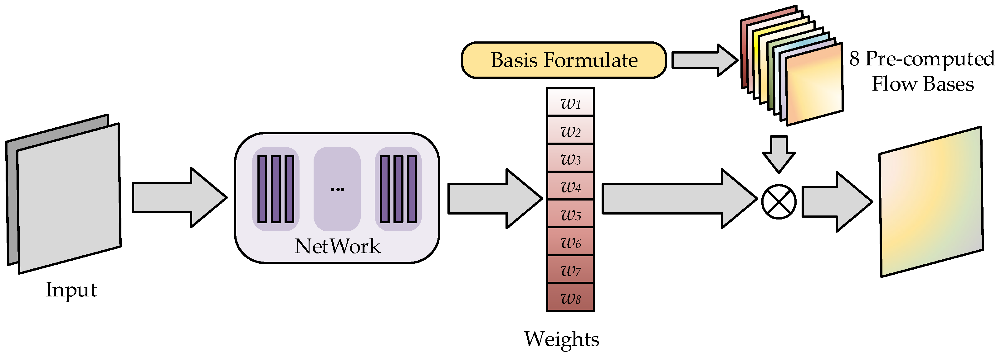
In 2021, Ye et al. [33] proposed a new unsupervised deep homography framework in 2021. They first introduced the idea of a homography flow representation, estimated by a weighted sum of eight predefined homography flow bases. Since homography contains only 8 degrees of freedom, which is far from the rank of the network features, they introduced a Low-Rank Representation (LRR) block. This design retains features related to the dominant motion while excluding irrelevant features. A Feature Identity Loss (FIL) was introduced to improve the model’s efficacy further, which ensured that the learned image features remained unchanged after distortion. In other words, the results should be consistent whether the warping operation or the feature extraction is done first. However, the method may fail in large baseline scenarios, and a single homography output may not be sufficient in real-world scenarios. In 2022, Hong et al. [77] proposed a new method called HomoGAN, which focuses homography estimation more on the principal plane. HomoGAN first constructs a multi-scale transformer network that predicts the homography from a pyramid of features in the input image in a coarse-to-fine manner. To impose coplanarity constraints, they introduce an unsupervised Generative Adversarial Network (GAN). The generator predicts the masks of the aligned regions, while the discriminator verifies that the two mask feature maps are induced by a single homography. The homography flow form provides a novel solution to homography matrices, which can handle the feature information brought by the dominant motion or related to the principal plane and opens up a new avenue for future research. Otherwise, except for the above two methods that used the homography flow representation of the homography matrix, the other methods used the 4-point parameterization form.

In 2017, Erlik et al. [78] presented a hierarchy of twin convolutional regression networks to estimate the homography between two images. The networks are stacked sequentially in this framework to reduce the estimation error progressively. Every convolutional network module autonomously extracts features from both images and then fuses these features to estimate the homography. Because of its iterative nature, the method does not require complex models, and a hierarchical arrangement of simple models can achieve high-performance homography estimation, which shows new paths to optimize the balance between complexity and performance. In 2018, Nguyen et al. [79] trained a neural network using pixel-wise photometric loss, which measures the pixel error between a warped input image and another image. This method allows unsupervised training without real labels. Compared to traditional methods, it is not only faster but also equal or better in accuracy and robustness to light variations. However, it does not fully account for the complexity of dealing with depth differences and moving objects in real-world applications. In 2019, Zhou et al. [80] proposed a neural network named STN-Homography based on a spatial transform network. The method aims to estimate the normalized homography matrix of image pairs directly. They designed hierarchical STN-homography and sequential STN-homography models with end-to-end training to reduce estimation error. This approach yielded dramatic improvements in accuracy and efficiency, providing new inspiration for unsupervised methods for researchers.

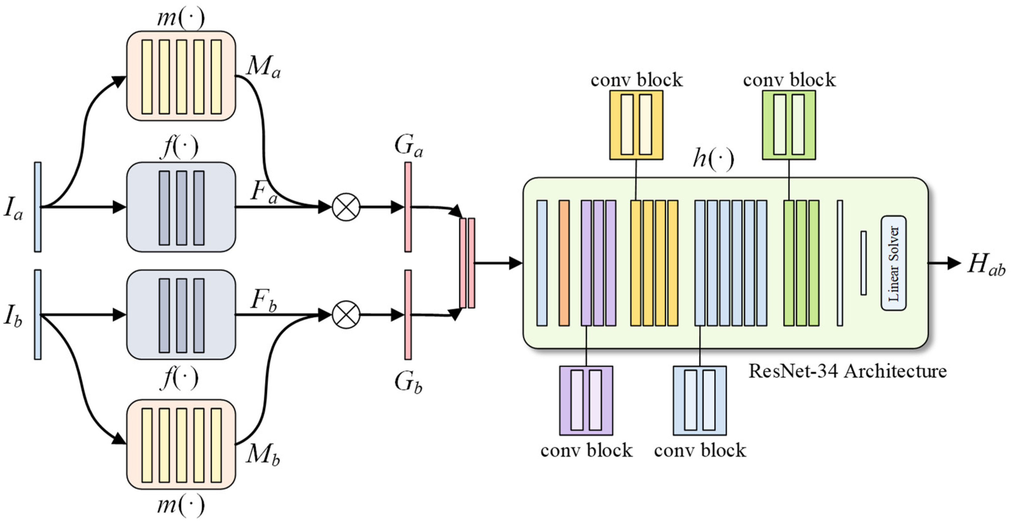
In 2020, Zhang et al. [81] designed a content-aware, unsupervised homography estimation method for image pairs with small baselines; its network structure is shown in Figure 8. For robust homography optimization, the method implicitly learns deep alignment features and a content-aware mask that helps the network select only reliable regions for homography estimation. Furthermore, learned features are used to compute the loss, while content-aware masks allow the network to focus on the regions that are important and representable. To optimize this network, they introduced a new triplet loss for unsupervised learning to optimize this network. Specifically, introducing content-aware masks has guided the design of future deep homography estimation networks. Numerous scholars have begun to realize that image masks can improve the performance of networks effectively and have begun to incorporate various types of attentional mechanisms into networks for robust homography estimation [82,83,84].

In 2020, Kharismawati et al. [85] proposed an unsupervised deep homography estimation method for agricultural aerial imagery. They improved the unsupervised CNN network of Nguyen et al. and used the video of maize nurseries imaged with a freely flown consumer-grade vehicle to train the network. This method can estimate the sequence of planar homography matrices of our corn fields from imagery without using metadata to correct estimation errors. It performs faster than the gold standard ASIFT algorithm while maintaining accuracy comparable to ASIFT. In 2021, Koguciuk et al. [86] proposed a bidirectional implicit Homography Estimation (biHomE) loss for unsupervised homography estimation. This method distinguishes homography estimation from representation learning for image comparison and enhances the robustness of homography estimation results to variations in illumination by minimizing the distance in feature space between the distorted image and the corresponding image. To combat the lack of robustness of traditional methods in low texture scenarios and the poor performance of deep learning-based methods in low overlap rate scenarios, Nie et al. [87] proposed a depth-aware multi-grid deep homography estimation network in 2021. This network achieves global to local parallax image alignment, overcoming the limitations of existing deep homography estimation methods. The method also designed a Contextual Correlation Layer (CCL) to extract the matching relationship, making the network better than the cost volume regarding performance, number of parameters, and speed. The method successfully overcomes the lack of robustness of traditional methods in low-texture scenes and the poor performance of deep learning-based methods in low-overlap scenes. However, the network structure and data size may limit the number of meshes for this network.

In 2022, Wu et al. [88] presented an unsupervised homography estimation algorithm incorporating a correction function. It employs a two-level network cascade structure, an idea similar to iteration. Each level of the network comprises an equivalent number of layers and parameters. The output homography matrix of the next network level is the residual of the true matrix and the sum of the previous output homography matrix. The method compensates the inputs of the next level network with the outputs of the previous level network, leading to the correction of the homography estimate. To tackle mis-correspondence due to appearance changes, relative motion between camera and object, and occlusion challenges, Zhang et al. [89] proposed a unified convolutional neural network model, HVC-Net. The model combines homography, visibility, and confidence and embeds them all into a Lucas-Kanade tracking pipeline to achieve accurate and robust planar object tracking of planar objects. This method can deal well with mismatches caused by such issues as changes in appearance, relative motion of camera and object, and occlusion, making homography estimation more widely applicable to object recognition and tracking. Nevertheless, due to the limitations of the LK-based method, the method sometimes suffers from the interference of similar occluding object factors.

In 2023, Hou et al. [30] proposed an unsupervised homography estimation method. Firstly, they constructed an unsupervised homography estimation method based on cascaded CNNs to solve the problem of low accuracy of existing unsupervised homography estimation methods. This method uses a two-stage cascade network structure and predicts the residuals of the overall homography at each stage. It can minimize the pixel intensity error between the two images and implements an unsupervised coarse-to-fine homography estimation. To address the issue of image homography under large parallax, Hou et al. [90] designed an unsupervised Multiscale Multi-stage based Content-Aware Homography Estimation method (MS2CA-HENet). This method uses images of different sizes as inputs in different stages to deal with different scales of homography transformations between images. Notably, they account for local and global features at each stage via a Self-attention Augmented Convolutional Network (SAC) and minimize the error residual at each stage to estimate the homography of large-displacement image pairs from coarse to fine.

Unlike supervised methods, unsupervised methods do not require labeled data but are more difficult to train and optimize. In particular, they face challenges in optimizing complex network structures and balancing performance. However, unsupervised learning still opens new research directions for deep learning-based homography estimation methods. In addition, a comprehensive analysis of unsupervised deep-learning homography estimation algorithms for single-source images is presented in

Table 4. Unsupervised homography estimation methods. The table provides details of the year of publication, core idea, advantages, and limitations for each method.

Method			Refer.	Year	Core Idea	Advantages	Limitations
Unsupervised	Homography Flow	Motion Basis Learning for Unsupervised Deep Homography Estimation with Subspace Projection	[33]	2021	Propose a homography flow representation.	Effectively achieved unsupervised optimization and more stable features are learned.	It is possible that it could lead to inaccuracies when applied to cases with large baselines.
		HomoGAN	[77]	2022	Propose a new approach for directing homography estimation towards the dominant plane.	Matching error is 22% lower than the previous state-of-the-art method.	Image pairs with large grayscale and contrast differences will cause the homography flow to become unstable.
	4-point Parameterization	Homography estimation from image pairs with hierarchical convolutional networks	[78]	2017	Introduce a hierarchy of twin convolutional regression networks.	High performance through the arrangement of simple models.	Sequential learning models must be used to handle the error propagation.
		Unsupervised deep homography: A fast and robust homography estimation model	[79]	2018	Neural networks are trained using photometric loss.	Achieve faster inference speed with better accuracy and robustness.	The robustness of occlusion was not studied.
		STN-Homography	[80]	2019	STN-homography was used to estimate the normalized homography directly.	The model meets real-time processing requirements.	Loss calculated directly on the intensity and uniformly on the image plane.
		Content-Aware Unsupervised Deep Homography Estimation	[81]	2020	Propose an unsupervised deep homography method with a new architecture design.	Designed for image pairs with small baselines, robustly optimizes homography.	Poor performance with large baseline images.
		Cornet	[85]	2020	Used the video of maize nurseries captured by a freely flown consumer-grade vehicle to train the network.	Faster than the gold standard ASIFT algorithm while maintaining accuracy.	Requires extra training data.
		Perceptual loss for robust unsupervised homography estimation	[86]	2021	Introduce a novel perceptual loss.	biHomE loss is beneficial for performance degradation from smaller to bigger viewpoint shifts.	The loss is only effective on scenes with small baselines and is prone to failure when there is a low overlap rate.
		Depth-aware multi-grid deep homography estimation with contextual correlation	[87]	2021	Design of a contextual correlation layer and introduction of a novel depth-aware shape-preserving loss.	Is better than the cost volume regarding performance, number of parameters, and speed.	Network structure and data size may limit the number of meshes.
		Sub-pixel Homography Matrix Estimation Based on Unsupervised Cascade	[88]	2022	An unsupervised homography estimation algorithm with correction function.	Has more accurate estimation capabilities.	During training and testing, local motion is used rather than global motion. Attention mechanism not introduced.
		HVC-Net	[89]	2022	Present a unified CNN model that considers homography, visibility, and confidence jointly.	Achieved excellent planar tracking performance on the public dataset, providing visibility masks.	The approach sometimes disturbed by the factor of occluded objects.
		Unsupervised Homography Estimation Based on Cascaded CNN	[30]	2023	Coarse-to-fine homography estimation of images using a two-stage cascade network structure.	It is robust and maintains good performance even when there is little overlap between the input images.	Difficulty in fully aligning image pairs with depth differences and parallax variations.
		MS2CA-HENet	[90]	2023	Use multi-scale input images for different stages to cope with different scales of transformations.	Lower error can be achieved when there are large displacement changes between corresponding points.	Need to introduce additional neural network structures to extract multi-scale feature maps.

.

Other methods. Besides the supervised and unsupervised methods discussed above, researchers have used other methods (e.g., self-supervised and semi-supervised) to tackle the task of homography estimation. Self-supervised algorithms can self-generate supervised signals for training, i.e., labels are automatically generated from unlabeled input data and used for training iterations. Compared to supervised and unsupervised methods, self-supervised methods effectively reduce the dependence on labeled data while increasing the use of unlabeled data, thus improving the robustness of the model. In 2019, Wang et al. [91] proposed the Self-Supervised Regression Network (SSR-Net). This method reduces the dependence on actual image annotations and uses a spatial pyramid pooling module to use contextual information to improve the quality of extracted features in each image. Furthermore, they chose the homography matrix representation rather than the 4-point parametrization to exploit reversibility constraints. In 2022, Li et al. [92] proposed the Self-Supervised Outlier Removal Network (SSORN), which incorporates a novel self-supervised loss function to remove noise in the image, mimicking the traditional outlier removal process. In 2023, Liu [13] et al. proposed a novel detector-free feature-matching method called Geometrized Transformer (GeoFormer). This method integrates GeoFormer into the LoFTR framework and trains end-to-end in a fully self-supervised manner. It can compute cross-attention diffusion regions in a focused manner and enhance local feature information through the Transformer.

Compared to self-supervised methods, which can automatically generate labeled data, semi-supervised learning requires training with both limited amounts of labeled data and large amounts of unlabeled data and attempts to use structural information in the unlabeled data to augment the learning process. Semi-supervised learning combines the advantages of both supervised and unsupervised methods and is more efficient on large-scale datasets. As a result, network models trained using semi-supervised methods have better generalization ability. In 2023, Jiang et al. [93] proposed a progressive estimation strategy. The strategy reconstructs the original homography by converting the large baseline homography into multiple intermediate homography terms and cumulatively multiplying these intermediate terms. Meanwhile, the method uses supervised and unsupervised losses to optimize intermediate homography and estimate large baseline homography without photometric losses. The approach effectively copes with the errors in homography estimation for large baselines, especially in the context of low image coverage and limited sensory field. Additionally, a comprehensive analysis of self-supervised and semi-supervised deep-learning homography estimation algorithms for single-source images is presented in

Table 5. Self-supervised and semi-supervised homography estimation methods. The table provides details of the year of publication, core idea, advantages, and limitations for each method.

Method			Refer.	Year	Core Idea	Advantages	Limitations
Other methods	Self-Supervised	SSR-Net	[91]	2019	Employ spatial pyramid pooling modules to enhance the quality of extracted features.	Relaxing the need for ground truth annotations.	The method cannot be directly using a 4-point parameterization.
		SSORN	[92]	2022	Develop a deep learning model that simulates all four phases in the traditional homography estimation.	Better performance in image pairs with a lot of noise.	Equipped with an outlier removal module that does not train well with supervised loss in paper.
		GeoFormer	[13]	2023	Integrate GeoFormer into the LoFTR framework.	Excellent performance on multiple real-world datasets.	If the coarse matches fail in the first place, GeoFormer shall fail.
	Semi-Supervised	Semi-supervised deep large-baseline homography estimation with progressive equivalence constraint	[93]	2023	Propose a progressive estimation strategy by converting large baseline homography.	Achieves state-of-the-art performance in large baseline scenarios.	Has limitations in the multi-plane sense.

.

3.2. Multimodel Image Homography Estimation Methods

Multi-source images, also known as multimodal images, typically refer to image data acquired using sensors with two or more different types of imaging mechanisms for the same scene or object. Such images comprise visible images, infrared images [94], hyperspectral images [95], optical Synthetic Aperture Radar (SAR) images [96], and Light Detection and Ranging (LiDAR) [97]. These different modality images can provide diverse and complementary feature information for the same scene or object [98]. However, traditional homography estimation methods based on features, such as SIFT and SURF, frequently lead to mismatching feature points when working with multimodal images due to significant modal differences between the images, resulting in poor performance or even failure of the algorithms. Recent studies have proposed applying deep learning techniques to tackle this issue. Deep learning-based methods for estimating homography in multi-source images follow three main ideas.

The first idea is to extract the features of different modal images using convolutional neural networks and further compute the homography matrix. In detail, a 4-point parameterization of the homography matrix is usually used as a regression value to achieve end-to-end multimodal image homography estimation. In 2022, Luo et al. [99] introduced a detail-aware deep homography estimation network to retain more detailed information in images. This method uses a shallow feature extraction network to select meaningful features from multilevel, multidimensional features that estimate the homography matrix. They additionally introduce a Detail Feature Loss (DFL) to better preserve detailed information and reduce the impact of unimportant features. This loss is calculated based on the refined features, which enables effective unsupervised learning.

The second idea is to transform the multimodal homography estimation problem into an approximate single-source one by transforming a given modal image into another one via a Generative Adversarial Network. To address modal and significant feature disparities between images, in 2022, Pouplin et al. [100] proposed a two-step approach designed for infrared and visible. They trained a GAN to learn a domain transfer function between the infrared and visible domains to reduce visual differences between images. Then, they applied a deep Siamese network to perform homography estimation in an unsupervised environment. This scheme effectively reduces the significant differences between different modal images, allowing common features to be robustly extracted and valid homography estimation. However, the training process of this method is cumbersome, and the GAN network may produce artifacts when transforming the images, affecting the final results.

The third idea combines the advantages of the two previous approaches: firstly, a convolutional neural network extracts shallow features. Secondly, it uses the GAN to optimize the homography matrix further. Considering the significant grey scale difference between infrared and visible and the low alignment accuracy, Luo et al. [73] proposed a GAN-based homography estimation method for infrared and visible. The method uses the Residual Dense Block (RDB) to construct the shallow feature extraction network that captures the deep features of the image. Then, the method introduces GAN to predict the homography matrix directly. The generator employs ResNet-34 as a backbone structure to predict the homography matrix. The discriminator is responsible for discriminating between the warped image and the target image. By generating an adversarial game between the generator and discriminator, the features between the warped image and the target image become closer, improving the homography estimation performance. Moreover, Luo et al. [74] improved on this basis. They have developed a simpler feature extractor network, which does not share weights, to extract detailed feature maps for infrared and visible. Furthermore, they designed a new generator. It uses an encoder-decoder structure to capture meaningful features at different scales and predict the homography matrix. Additionally, Wang et al. [101] proposed a Feature Correlation Transformer (FCTrans) method to explicitly guide feature matching, enabling homography estimation for infrared and visible. Its network structure is shown in Figure 9. The method first proposes a feature patch as the basic unit of correlation calculation, effectively mitigating the modal differences between infrared and visible. Then, a novel cross-image attention mechanism identifies the correlation between different modal images, thus achieving the source-to-target image mapping in the feature dimension and transforming the multi-source images homography estimation problem into a single-source images problem. Finally, they developed a Feature Correlation Loss (FCL) to encourage the network to learn a differentiated target feature map for better mapping source-to-target images. This approach successfully reduced the homography estimation errors caused by imaging differences in the multi-source images and substantially boosted the accuracy of homography estimation for multi-source images. Then, Wang et al. [102] proposed a new coarse-to-fine strategy for homography estimation. This strategy obtains multi-scale feature maps by different stages in the regression network, avoiding the need to introduce additional neural networks in the traditional coarse-to-fine strategy. Furthermore, they developed a Local Correlation Transformer (LCTrans) that captures the intrinsic connections between features for better progressive refinement of the homography matrix.

The study of multimodal image homography estimation algorithm enables this technique to obtain more robust and accurate results in various complex image environments, which can better satisfy the increasingly complex needs of different application areas in reality. Moreover, these thoughts provide essential guidance for developing multimodal image processing techniques in other areas of computer vision.

Table 6. Deep learning-based methods for multimodal homography estimation. The table lists the year of publication, core idea, advantages, and limitations of each method.

Method		Refer.	Year	Core Idea	Advantages	Limitations
Deep Learning	Detail-Aware Deep Homography Estimation for Infrared and Visible Image	[99]	2022	Proposed a detail-aware deep homography estimation network to obtain detailed information.	Dramatically improved performance of PME and AFFR metrics on real datasets.	Shallow feature extraction methods in multi-source images still need improvement.
	Multimodal Deep Homography Estimation Using a Domain Adaptation Generative Adversarial Network	[100]	2022	Propose a two-stage approach targeting infrared and visible.	Outperforms some baselines and deep homography methods of the time.	GAN may produce artifacts such as blurring or hallucinations, which may lead to inaccuracy in feature localization.
	Infrared and Visible Homography Estimation Method Based on GAN	[73]	2023	A GAN-based method for estimating homography in infrared and visible.	Effectively improve homography estimation performance.	Black borders may be produced when images are warped.
	HomoMGAN	[74]	2023	Developed an infrared and visible homography estimation method based on multiscale GAN.	Outperforms current state-of-the-art methods both qualitatively and quantitatively.	Limited performance of homography estimation in low-light scenarios.
	FCTrans	[101]	2023	Propose a feature correlation transformer method to guide feature matching.	Homography estimation performance dramatically enhanced.	It might need further optimization and adjustment when processing images in large-baseline scenarios.
	LCTrans	[102]	2023	Design a novel coarse-to-fine strategy to obtain multi-scale feature maps and enable the progressive refinement of the homography matrix.	No need to introduce additional neural networks to obtain multi-scale feature maps, and avoids complex matrix fusion operations.	Does not perform as well as some comparative methods in some challenging scenarios.

comprehensively analyzes multimodel Image homography estimation algorithms. The table lists the year of publication, core idea, advantages, and limitations of each method.

4. Evaluation Metrics

Homography estimation is a critical task in computer vision, focusing on finding the geometric relationship between two images. Real-world data often deviate from the theoretical model due to internal and external camera parameters, image noise, and other confounding factors, making homography estimation challenging. To validate the performance of different algorithms on this task, it is necessary to have a set of precise and reliable evaluation metrics. Such metrics not only offer researchers an assessment of algorithm accuracy but also help them understand the potential weaknesses of the algorithms and provide direction for future research. This section will discuss the usual evaluation metrics for homography estimation.

4.1. Relative Measurement Error

The Relative Measurement Error (RME) [45] is a metric defined by Zeng et al. in 2008 for evaluating homography estimation models based on line features. Firstly, generate a reference template and select 100 points equally spaced on each side of the template. These 100 image points on each side are fitted to a line using a least-squares algorithm. Then, estimate the homography from the reference plane to the image plane and map these image points to Euclidean space. Finally, the distance between the two sets of spatial points can be determined. To obtain statistically significant results, randomly select 100 pairs of such spatial points in each test and estimate the distance between them from their corresponding image points. The relative measurement error can be defined as:

$$\mathrm{R}\mathrm{M}\mathrm{E}=\left(\frac{\left|D_t-D_e\right|}{D_t}\times 100\right)\%$$

(11)

where $D_t$ is the true distance and $D_e$ is the predicted distance.

4.2. Average Corner Error

The Average Corner Error (ACE) [31] is acquired by calculating the $l_2$ distance between the ground truth and estimated corner locations. It is mainly used to evaluate the performance of supervised homography estimation methods. A lower ACE value means better homography estimation performance. ACE is defined as:

$$\mathrm{A}\mathrm{C}\mathrm{E}=\frac{{\sum }_{i=1}^4{\left||x_i-y_i|\right|}_2}{4}$$

(12)

where $x_i$ and $y_i$ represent the corners obtained by converting the corner corners $i$ through the ground-truth homography and estimated homography transformations, respectively.

4.3. Point Matching Error

Point Matching Errors (PME) [99] are calculated by averaging the $l_2$ distance between warped source points and target points, primarily used to evaluate the performance of unsupervised homography estimation methods. The smaller the value of PME, the better the homography estimation performance. PME can be expressed as:

$$\mathrm{P}\mathrm{M}\mathrm{E}=\frac{{\sum }_{i=1}^N{\left||x_i-y_i|\right|}_2}{N}$$

(13)

where $x_i$ denotes point $i$ transformed by the homography matrix; $y_i$ represents the manual annotation match point corresponding to point $i$; $N$ is the number of manual annotation match points.

4.4. Root Mean Square Error

Root Means Square Error (RMSE) [103] is used to measure the difference between the predicted value and the true value. In homography estimation, the RMSE is often used to quantify the reprojection error. This is the error between the positions of the mapped points and the actual points after mapping the points in one image to another using an estimated homography matrix. The lower the RMSE, the closer the estimated homography matrix is to the true homography matrix, while the higher the RMSE, the greater the error. The RMSE can be written as:

$$\mathrm{R}\mathrm{M}\mathrm{S}\mathrm{E}=\sqrt{\frac{1}{N}\sum _{i=1}^N{‖{\overline{X}}_i^{\prime }-H_{est}{\overline{X}}_i‖}_2^2}$$

(14)

where $({\overline{X}}_i, {\overline{X}}_i^{\prime })$ denotes the true corresponding point; $N$ is the number of corresponding points; $H_{est}$ represents the estimated homography matrix.

4.5. Alignment Error

Alignment Error (AE) [104] is a metric used to measure the error between the predicted position and the real position. The error is calculated by employing four reference points, which are comprised of the target’s four corner points. AE is defined as the root-mean-square (RMS) distance between the estimated positions of these corner points and its true position, as shown:

$$\mathrm{A}\mathrm{E}=\sqrt{\frac{{\sum }_{i=1}^4{\left(x_i-x_i^{*}\right)}^2}{4}}$$

(15)

where $x_i$ is the estimated position of the point and $x_i^{*}$ is the ground-truth position.

4.6. Homography Discrepancy

The Homography Discrepancy (HD) [104] measures the difference between the true homography matrix $H^{*}$ and the predicted homography matrix $H$, which can be expressed as shown:

$$\mathrm{H}\mathrm{D}(H^{*},H)=\frac{\sum _{i=1}^4{\left||c_i-(H^{*}{H}^{-1})\left(c_i\right)|\right|}_2}{4}$$

(16)

where $c_i$ denotes the corners of the square, and the value of $HD$ is 0 when $H$ and $H^{*}$ are equal.

4.7. Mutual Information

Mutual Information (MI) [99] reflects the correlation degree by calculating the entropy and joint entropy of the warped and ground-truth images. MI determines the accuracy of homography estimation by measuring the similarity between the two images in terms of grey-scale distribution. The greater the MI value, the more similar the two images are, and the homography estimation is more accurate. It can be expressed as:

$$\mathrm{M}\mathrm{I}\left(x, y\right)=H\left(x\right)+H\left(y\right)-H(x, y)$$

(17)

where $x$ and $y$ represent warped and ground-truth images; $H(\cdot )$ and $H(x, y)$ are the calculation functions of entropy and joint entropy, respectively.

4.8. Structural Similarity

Structural Similarity (SSIM) [74] is a metric to measure the similarity between two images. It has a range of values ranging from 0 to 1. When applied to homography estimation, SSIM helps us evaluate the similarity between a target image and a source image after homography transformation. The higher the SSIM value, the higher the similarity and the more accurate the homography estimation. It is calculated as shown:

$$\mathrm{S}\mathrm{S}\mathrm{I}\mathrm{M}\left(x,y\right)=\frac{\left(2{\mu }_x{\mu }_y+c_1\right)\left(2{\sigma }_{xy}+c_2\right)}{\left({\mu }_x^2+{\mu }_y^2+c_1\right)\left({\sigma }_x^2+{\sigma }_y^2+c_2\right)}$$

(18)

where $x$ and $y$ represent the warped and ground-truth images; ${\mu }_x$ and ${\mu }_y$ are the average of all pixels in $x$ and $y$; ${\sigma }_x$ and ${\sigma }_y$ stand for the standard deviations of $x$ and $y$, respectively; ${\sigma }_{xy}$ denotes the covariance between two images; $c_1$ and $c_2$ represent constants to maintain stability.

4.9. Peak Signal-to-Noise Ratio

Peak Signal-to-Noise Ratio (PSNR) [99] is a metric that reflects the overall greyscale difference between two images. A higher PSNR value indicates that the greyscale difference between two images is smaller, and the image pair is more similar. The calculation of PSNR can be expressed as shown:

$$\mathrm{P}\mathrm{S}\mathrm{N}\mathrm{R}\left(x, y\right)=10{log}_{10}\frac{MN{\left(2^k-1\right)}^2}{\sum _{i=1}^M\sum _{j=1}^N{\left(x\left(i,j\right)-y\left(i,j\right)\right)}^2}$$

(19)

where $x$ and $y$ denote the warped image and the real image, respectively; $i$ and $j$ represent the pixel positions in the rows and columns of the image; and $k$ is the number of bits in each sample value.

4.10. Adaptive Feature Registration Rate

Adaptive Feature Registration Rate (AFRR) [99] uses SIFT to extract image feature points adaptively, avoiding manual annotation of many feature match pairs. The metric first takes the Euclidean distance $d_i$ between matched feature points as a judgment quantity and sets a threshold $\epsilon$ as the criterion for mismatching. Only if $d_i$ is less than $\epsilon$ will it be included in the next step of the judgment and recorded as $d_i^{\prime }$. Then, set another threshold $\mu$, and the feature match is considered accurate only if $d_i^{\prime }$ is less than $\mu$. Otherwise, it is considered inaccurate. Finally, the AFRR is obtained by calculating the proportion of feature matches that are considered accurate across all judgment ranges. Its calculation formula is given:

$$\mathrm{A}\mathrm{F}\mathrm{R}\mathrm{R}=\frac{1}{N}\sum _{i=1}^N\mu \left(d_i^{\prime }\right)$$

(20)

where $\mu \left(d_i^{\prime }\right)$ stand for the number of matches judged to be accurate under the threshold $\mu$; $N$ is the number of matching corresponding feature points satisfying the threshold $\epsilon$. In the experiment, the threshold $\epsilon$ was set to 10, and $\mu$ was set to 6.

Table 7. Evaluation indicators and meaning. This table lists the evaluation metrics for homography estimates, the calculation formulae, the evaluation criteria, and the cited literature.

Evaluation Metric		Calculate	Criteria	Cited
RME	Relative Measurement Error	$RME=\left(\frac{\left|D_t-D_e\right|}{D_t}\times 100\right)\%$	The smaller, the better.	[45]
ACE	Average Corner Error	$ACE=\frac{{\sum }_{i=1}^4{\left||x_i-y_i|\right|}_2}{4}$	The smaller, the better.	[31,63,68,69,71,73,74,77,99,101]
PME	Point Matching Errors	$PME=\frac{{\sum }_{i=1}^N{\left||x_j-y_j|\right|}_2}{N}$	The smaller, the better.	[33,81,93,99,101]
RMSE	Root Mean Square Error	$RMSE=\sqrt{\frac{1}{N}{\displaystyle \sum _{i=1}^N}{‖{\overline{X}}_i^{\prime }-H_{est}{\overline{X}}_i‖}_2^2}$	The smaller, the better.	[14,71,79,85,87,103]
AE	Alignment Error	$AE=\sqrt{\frac{{\sum }_{i=1}^4{\left(X_{Ti}-X_{GTi}\right)}^2}{4}}$	The smaller, the better.	[89]
HD	Homography Discrepancy	$HD(H^{*},H)=\frac{\sum _{i=1}^4{\left||c_i-(H^{*}{H}^{-1})\left(c_i\right)|\right|}_2}{4}$	The smaller, the better.	[89]
MI	Mutual Information	$\mathrm{M}\mathrm{I}\left(x, y\right)=H\left(x\right)+H\left(y\right)-H(x, y)$	It is necessary to determine whether the degree of similarity meets the threshold requirements.	[99]
SSIM	Structural Similarity	$SSIM\left(x,y\right)=\frac{\left(2{\mu }_x{\mu }_y+c_1\right)\left(2{\sigma }_{xy}+c_2\right)}{\left({\mu }_x^2+{\mu }_y^2+c_1\right)\left({\sigma }_x^2+{\sigma }_y^2+c_2\right)}$	The closer it is to 1, the more accurate it is.	[67,73,99]
PSNR	Peak Signal-to-Noise Ratio	$PSNR\left(x, y\right)=10{log}_{10}\frac{MN{\left(2^k-1\right)}^2}{\sum _{i=1}^M\sum _{j=1}^N{\left(x\left(i,j\right)-y\left(i,j\right)\right)}^2}$	The larger, the better.	[67,99]
AFRR	Adaptive Feature Registration Rate	$AFRR=\frac{1}{N}{\displaystyle \sum _{i=1}^N}{d}_i^{\prime }$	The higher, the better.	[99]

lists the significance of the evaluation metrics for the estimation of homographies, the evaluation criteria, the calculation formulae, and the cited literature.

5. Applications Fields

In computer vision, the homography estimation technique is indispensable for handling complex visual tasks efficiently and accurately. This technique proves its unique application value in image stitching, augmented reality, object recognition, and tracking.

In image stitching [105,106,107,108,109,110,111], homography estimation enables seamless fusion by accurately estimating the geometric transformation relationships between images from different viewpoints. This technique allows for synthesizing images from multiple views, providing a more comprehensive perspective and deeper analysis, with important implications for work such as landscape photography and 3D digital reconstruction of cultural heritage. In Virtual Reality (VR) [112] and Augmented Reality (AR) [113,114,115], homography estimation is also crucial. It provides strong support for creating realistic and immersive virtual environments and enhancing the realism and immersion of AR experiences, especially in complex and dynamic environments such as education, entertainment, and personnel training.

In the medical imaging domain [116,117,118], homography estimation applications have expanded, including tumor motion tracking [116], iterative matching of X-ray images [117], and multimodal medical image alignment (e.g., MRI and CT images) [118]. These applications are vital for improving the accuracy of medical diagnosis and treatment. In object recognition and tracking [4,119,120,121,122], homography estimation helps to accurately recognize and track objects in dynamic environments, facilitating the development of self-driving cars and security surveillance systems. In-camera calibration [123,124,125] and perspective correction [126,127], homography estimation can effectively correct the visual aberration caused by different photography angles, thus dramatically improving the accuracy and reliability of the recognition system. In gesture recognition [128], the application of homography estimation offers technical support for developing more intuitively operable human–computer interaction interfaces, making the process of human–computer interaction more natural and compatible with human behavior.

Furthermore, homography estimation has shown irreplaceable importance in developing Simultaneous Localization and Mapping (SLAM) [129,130] techniques, especially in indoor environments without GPS support. It plays a central role in environmental mapping and path planning and provides critical visual information for automatic navigation systems. In video stabilization [131,132,133], homography estimation reduces image jitter caused by device motion, improving video quality.

Homography estimation is an advanced computer vision technique demonstrating its unique value and widely applicable potential in several fields. Even facing image pairs with large displacements and illumination variations, the homography estimation system handles this challenge well [134]. It plays an essential role in solving complex vision problems and opens up new directions for future technological development. With continuing research, homography estimation will become more critical in future computer vision research and practice.

Table 8. Fields of application of homography estimation and related articles.

Application Fields	Refer.
image stitching	[105,106,107,108,109,110,111]
virtual reality and augmented reality	[112,113,114,115]
medical imaging domain	[116,117,118]
object recognition and tracking	[4,119,120,121,122]
camera calibration	[123,124,125]
perspective correction	[126,127]
gesture recognition	[128]
SLAM	[129,130]
video stabilization	[131,132,133]

lists the fields of application of homography estimation techniques.

6. Challenges and Perspectives

Homography estimation plays a significant role in many application scenarios but also brings many problems and challenges. This section will explore the challenges and prospects of homography estimation in single-source and multimodal images.

6.1. Challenges and Prospects of Single-Source Image Homography Estimation

Homography estimation is an important research task in computer vision. Single-source images refer to image transformations from the same sensor but are caused by changes in viewpoint due to different times or locations. In this instance, Homography estimation is concerned with estimating the geometric transformation between two views of the same image. Although this task may be simple in theory, in practice, it is difficult due to various factors such as illumination, occlusion, and noise. With time, homography estimation methods have gradually shifted from traditional feature-based strategies to deep learning-based methods. To understand the strengths and weaknesses of these methods in estimating the homography of single-source images, we will explore the challenges and possible prospects of these methods.

Feature-based methods are mainly based on the extraction and matching of image features. These methods have achieved good results in many practical applications but face challenges in some specific scenarios. Firstly, extracting and matching feature points may encounter challenges in complex and dynamically changing backgrounds. Specifically, the accuracy and robustness of feature matching can be challenged when the image changes in scale, rotation, illumination, and viewpoint. Additionally, selecting suitable feature descriptors for augmenting the robustness of matching presents a difficulty.

Despite the significant advancements achieved by deep learning methods in estimating homography, challenges remain. Supervised methods require synthetic examples with ground-truth labels to train the network, but large amounts of training data with ground-truth labels are difficult to obtain in practice. Meanwhile, the training data of supervised methods lacks real depth differences, leading to a limited ability to generalize to real images and reducing the accuracy of homography estimation. Unlike supervised learning, unsupervised learning does not require labeled data, but its training and optimization process is much more complex. Choosing the suitable loss function, ensuring the stability of the model, and dealing with unbalanced data distributions are all problems that need to be addressed using such methods. Researchers are trying to find more effective and robust solutions to these challenges, both feature-based and deep learning-based approaches.

As technology progresses, feature-based methods have great potential for development. The performance of such methods can be improved by new feature descriptors, more efficient matching algorithms, and global information strategies. Furthermore, combining deep learning and traditional methods is a promising research direction, which may provide more accurate and robust results for homography estimation.

As deep learning techniques continue to evolve, the structure of the model and the training strategy will be optimized, and we can expect supervised methods to achieve better performance in homography estimation. Techniques such as data augmentation, transfer learning, and semi-supervised learning are expected to solve the problem of insufficient data and overfitting, thus improving the performance of such methods. Unsupervised learning provides new research directions for homography estimation. Using new network structures and loss functions, combined with traditional methods and strategies, can improve the performance of such methods. With more unsupervised learning algorithms and techniques being proposed, we can expect even greater future breakthroughs in this type of approach.

Homography estimation is a field full of challenges and opportunities. With research and technological advances, we expect to achieve more accurate, faster, and robust homography estimation methods.

6.2. Challenges and Prospects of Multimodal Image Homography Estimation

Multimodal images generally refer to image data acquired by sensors with two or more different types of imaging mechanisms. This data acquisition method is common in remote sensing, medical imaging, and robotic perception domains. Multimodal image homography estimation is concerned with estimating the geometric transformations between different modalities of images to achieve alignment between Multimodal images. This estimation task becomes increasingly complex as the differences between different modalities increase. In this section, we will discuss the challenges and perspectives of this problem.

Significant differences in appearance and structure between multimodal images could make it difficult for feature-based methods to extract and match features. For instance, infrared and visible features may differ significantly. Therefore, extracting common and robust features from these images and performing effective matching are challenging problems [135].

Deep learning brings new challenges to multimodal image homography estimation. Firstly, designing network structures that can effectively handle different modal images is an important issue. Secondly, training a model that can differentiate and adapt to various modalities is challenging due to the significant differences between modalities. Otherwise, acquiring sufficient labeled data to train deep learning models is still a problem that needs to be overcome.

While facing these challenges, homography estimation for multimodal images has excellent potential for future development as technology advances and research intensifies.

With the advancement of computer vision and image processing techniques, further progress is expected in feature-based homography estimation methods for multimodal images. In the case of multimodal images, it is necessary to reconsider the feature extraction and matching strategy to ensure that robust matches can be found in all modal differences. Future research may focus on developing new feature descriptors that capture common features across different modalities and align them. Moreover, combining deep learning with traditional feature extraction methods can be an effective strategy, using deep networks to improve the performance of traditional features. Meanwhile, new algorithms and frameworks will be proposed to integrate information from different modalities better to address the feature fusion problem in multimodality.

Deep learning provides new opportunities for multimodal image homography estimation. For this particular problem, deep learning methods must cleverly fuse data from different sensors. Future research may explore how to fuse information from different modalities better to improve the accuracy of homography estimates. Adaptive and modality-invariant feature extraction will be emphasized to capture cross-modal commonalities and exclude modality-specific differences. In addition, considering the complexity of multimodal data, using multi-task learning and knowledge distillation techniques to utilize the complementary information between modalities fully will become a research hotspot.

In summary, although there are numerous challenges when estimating homography for multimodal images, it still has a promising future, driven by continuous research and technological advances. We expect more accurate and robust multimodal image homography estimation methods to be achieved.

7. Conclusions

In this paper, we comprehensively review the development history of homography estimation techniques and systematically analyze and evaluate different types of methods, covering the advantages and limitations of the methods and their related evaluation metrics. First, we explore the basic principles and matrix representation of homography estimation and then discuss feature-based and deep learning-based methods for single-source and multi-source images, respectively. Early studies focus on feature-based methods such as SIFT, SURF, and ORB. These methods perform well in specified scenarios, but in complex or changing environments, hand-crafted feature descriptors are insufficient in efficiency and accuracy in identifying and extracting features. Consequently, scholars have begun to employ neural networks to implement the feature extraction or matching steps in traditional methods to overcome these limitations.

Currently, homography estimation research relies on end-to-end deep learning methods, which include supervised, unsupervised, self-supervised, and semi-supervised methods. These methods can automatically learn and extract image features, providing greater accuracy and robustness when dealing with complex and varied images. Finally, we provide an in-depth discussion of the applications of homography estimation techniques and their challenges. Moreover, we look forward to their application prospects. While existing homography estimation techniques have achieved excellent results, there are still many challenges in practical use, such as the parallax problem in real scenes and the limitations of a single homography matrix in aligning the whole image.

References

1. Chen, P.; Peng, Z.; Li, D.; Yang, L. An improved augmented reality system based on AndAR. J. Vis. Commun. Image Represent. 2016, 37, 63–69. [Google Scholar] [CrossRef]
2. Gao, Q.H.; Wan, T.R.; Tang, W.; Chen, L. A stable and accurate marker-less augmented reality registration method. In Proceedings of the 2017 International Conference on Cyberworlds (CW), Chester, UK, 20–22 September 2017; pp. 41–47. [Google Scholar]
3. Skinner, P.; Zollmann, S. Localisation for augmented reality at sport events. In Proceedings of the 2019 International Conference on Image and Vision Computing New Zealand (IVCNZ), Dunedin, New Zealand, 2–4 December 2019; pp. 1–6. [Google Scholar]
4. Lotfian, S.; Foroosh, H. View-invariant object recognition using homography constraints. In Proceedings of the 2017 IEEE International Conference on Image Processing (ICIP), Beijing, China, 17–20 September 2017; pp. 605–609. [Google Scholar]
5. Ding, C.; Tao, D. Pose-invariant face recognition with homography-based normalization. Pattern Recognit. 2017, 66, 144–152. [Google Scholar] [CrossRef]
6. Li, N.; Xu, Y.; Wang, C. Quasi-homography warps in image stitching. IEEE Trans. Multimed. 2017, 20, 1365–1375. [Google Scholar] [CrossRef]
7. Xiang, T.Z.; Xia, G.S.; Zhang, L. Image stitching using smoothly planar homography. In Proceedings of the Chinese Conference on Pattern Recognition and Computer Vision (PRCV), Guangzhou, China, 23–26 November 2018; pp. 524–536. [Google Scholar]
8. Li, Y.; Tofighi, M.; Monga, V. Robust alignment for panoramic stitching via an exact rank constraint. IEEE Trans. Image Process. 2019, 28, 4730–4745. [Google Scholar] [CrossRef]
9. Bouchiha, R.; Besbes, K. Comparison of local descriptors for automatic remote sensing image registration. Signal Image Video Process. 2015, 9, 463–469. [Google Scholar] [CrossRef]
10. Su, H.R.; Lai, S.H. Non-rigid registration of images with geometric and photometric deformation by using local affine Fourier-moment matching. In Proceedings of the IEEE Conference on Computer Vision and Pattern Recognition, Boston, MA, USA, 7–12 June 2015; pp. 2874–2882. [Google Scholar]
11. Quenzel, J.; Horn, J.; Houben, S.; Behnke, S. Keyframe-based photometric online calibration and color correction. In Proceedings of the 2018 IEEE/RSJ International Conference on Intelligent Robots and Systems (IROS), Madrid, Spain, 1–5 October 2018; pp. 1–8. [Google Scholar]
12. Skinner, K.A.; Zhang, J.; Olson, E.A.; Johnson-Roberson, M. Uwstereonet: Unsupervised learning for depth estimation and color correction of underwater stereo imagery. In Proceedings of the 2019 International Conference on Robotics and Automation (ICRA), Montreal, QC, Canada, 20–24 May 2019; pp. 7947–7954. [Google Scholar]
13. Liu, J.; Li, X. Geometrized Transformer for Self-Supervised Homography Estimation. In Proceedings of the IEEE/CVF International Conference on Computer Vision, Paris, France, 2–6 October 2023; pp. 9556–9565. [Google Scholar]
14. Zhou, H.; Hu, W.; Li, Y.; He, C.; Chen, X. Deep Homography Estimation With Feature Correlation Transformer. In Proceedings of the 2023 IEEE International Conference on Multimedia and Expo (ICME), Brisbane, Australia, 10–14 July 2023; pp. 1397–1402. [Google Scholar]
15. Mohammed, H.M.; El-Sheimy, N. A Descriptor-less Well-Distributed Feature Matching Method Using Geometrical Constraints and Template Matching. Remote Sens. 2018, 10, 747. [Google Scholar] [CrossRef]
16. Liu, J.; Liang, A.; Zhao, E.; Pang, M.; Zhang, D. Homography Matrix-Based Local Motion Consistent Matching for Remote Sensing Images. Remote Sens. 2023, 15, 3379. [Google Scholar] [CrossRef]
17. Lin, B.; Xu, X.; Shen, Z.; Yang, X.; Zhong, L.; Zhang, X. A Registration Algorithm for Astronomical Images Based on Geometric Constraints and Homography. Remote Sens. 2023, 15, 1921. [Google Scholar] [CrossRef]
18. Ji, J.; Pan, F.; Wang, X.; Tang, J.; Pu, B. An end-to-end anti-shaking multi-focus image fusion approach. Image Vis. Comput. 2023, 137, 104788. [Google Scholar] [CrossRef]
19. Son, D.-M.; Kwon, H.-J.; Lee, S.-H. Visible and Near Infrared Image Fusion Using Base Tone Compression and Detail Transform Fusion. Chemosensors 2022, 10, 124. [Google Scholar] [CrossRef]
20. Huang, Y.; Zhu, M.; Chen, T.; Zheng, Z. Robust homography-based visual servo control for a quadrotor UAV tracking a moving target. J. Frankl. Inst.-Eng. Appl. Math. 2023, 360, 1953–1977. [Google Scholar] [CrossRef]
21. Lowe, D.G. Distinctive image features from scale-invariant keypoints. Int. J. Comput. Vis. 2004, 60, 91–110. [Google Scholar] [CrossRef]
22. Bay, H.; Tuytelaars, T.; Gool, L.V. Surf: Speeded Up Robust Features. In Proceedings of the European Conference on Computer Vision, Graz, Austria, 7–13 May 2006; pp. 404–417. [Google Scholar]
23. Rublee, E.; Rabaud, V.; Konolige, K.; Bradski, G. ORB: An Efficient Alternative to SIFT or SURF. In Proceedings of the 2011 International Conference on Computer Vision, Barcelona, Spain, 6–13 November 2011; pp. 2564–2571. [Google Scholar]
24. Tan, W.; Tiwari, P.; Pandey, H.M.; Moreira, C.; Jaiswal, A.K. Multimodal medical image fusion algorithm in the era of big data. Neural Comput. Appl. 2020, 1–21. [Google Scholar] [CrossRef]
25. Ye, Y.; Bruzzone, L.; Shan, J.; Bovolo, F.; Zhu, Q. Fast and robust matching for multimodal remote sensing image registration. IEEE Trans. Geosci. Remote Sens. 2019, 57, 9059–9070. [Google Scholar] [CrossRef]
26. Zhang, Z. A flexible new technique for camera calibration. IEEE Trans. Pattern Anal. Mach. Intell. 2000, 22, 1330–1334. [Google Scholar] [CrossRef]
27. Agarwal, A.; Jawahar, C.V.; Narayanan, P.J. A Survey of Planar Homography Estimation Techniques; Technical Report; International Institute of Information Technology: Hyderabad, India, 2005. [Google Scholar]
28. Abdel-Aziz, Y.I.; Karara, H.M. Direct liner transformation from comparator into object space coordinates in close-range photogrmmetry. In Proceedings of the Symposium on Close-Range Photogrammetry, Falls Church, VA, USA; 1971; pp. 1–18. [Google Scholar]
29. Golub, G.H.; Reinsch, C. Singular value decomposition and least squares solutions. In Handbook for Automatic Computation: Volume II: Linear Algebra Berlin; Springer: Berlin/Heidelberg, Germany, 1971; pp. 134–151. [Google Scholar]
30. Hou, B. A Study of Image Homography Estimation Based on Unsupervised Learning. Master’s Thesis, Yantai University, Yantai, China, 2023. (In Chinese). [Google Scholar]
31. DeTone, D.; Malisiewicz, T.; Rabinovich, A. Deep image homography estimation. arXiv 2016, arXiv:1606.03798. [Google Scholar]
32. Bai, Y. Research on Homography Estimation Based on Siamese Neural Network. Master’s Thesis, Harbin Institute of Technology, Shenzhen, China, 2021. (In Chinese). [Google Scholar]
33. Ye, N.; Wang, C.; Fan, H.; Liu, S. Motion Basis Learning for Unsupervised Deep Homography Estimation with Subspace Projection. In Proceedings of the IEEE/CVF International Conference on Computer Vision, Montreal, QC, Canada, 10–17 October 2021; pp. 13117–13125. [Google Scholar]
34. Wang, C.F. Research on Homography Transformation Estimation Based on Convolutional Neural Network and Its Application. Master’s Thesis, Zhengzhou University, Zhengzhou, China, 2021. (In Chinese). [Google Scholar]
35. Chum, O.; Matas, J. Homography estimation from correspondences of local elliptical features. In Proceedings of the 21st International Conference on Pattern Recognition (ICPR2012), Tsukuba, Japan, 11–15 November 2012; pp. 3236–3239. [Google Scholar]
36. Liu, S.; Wang, H.; Wei, Y.; Pan, C. BB-homography: Joint binary features and bipartite graph matching for homography estimation. IEEE Trans. Circuits Syst. Video Technol. 2014, 25, 239–250. [Google Scholar] [CrossRef]
37. Yan, Q.; Xu, Y.; Yang, X.; Nguyen, T. HEASK: Robust homography estimation based on appearance similarity and keypoint correspondences. Pattern Recognit. 2014, 47, 368–387. [Google Scholar] [CrossRef]
38. Zhao, C.; Zhao, H. Accurate and robust feature-based homography estimation using HALF-SIFT and feature localization error weighting. J. Vis. Commun. Image Represent. 2016, 40, 288–299. [Google Scholar] [CrossRef]
39. Barath, D.; Kukelova, Z. Homography from two orientation-and scale-covariant features. In Proceedings of the IEEE/CVF International Conference on Computer Vision, Seoul, Republic of Korea, 27 October–2 November 2019; pp. 1091–1099. [Google Scholar]
40. Suárez, I.; Sfeir, G.; Buenaposada, J.M.; Baumela, L. BEBLID: Boosted efficient binary local image descriptor. Pattern Recognit. Lett. 2020, 133, 366–372. [Google Scholar] [CrossRef]
41. Barclay, A.; Kaufmann, H. FT-RANSAC: Towards robust multi-modal homography estimation. In Proceedings of the 2014 8th IAPR Workshop on Pattern Reconition in Remote Sensing, Stockholm, Sweden, 24 August 2014; pp. 1–4. [Google Scholar]
42. Barath, D.; Matas, J.; Noskova, J. MAGSAC: Marginalizing sample consensus. In Proceedings of the IEEE/CVF Conference on Computer Vision and Pattern Recognition, Long Beach, CA, USA, 16–20 June 2019; pp. 10197–10205. [Google Scholar]
43. Rodríguez, M.; Facciolo, G.; Morel, J.M. Robust homography estimation from local affine maps. Image Process. Line 2023, 13, 65–89. [Google Scholar] [CrossRef]
44. Dubrofsky, E.; Woodham, R.J. Combining line and point correspondences for homography estimation. In Proceedings of the International Symposium on Visual Computing, Las Vegas, NV, USA, 1–3 December 2008; pp. 202–213. [Google Scholar]
45. Zeng, H.; Deng, X.; Hu, Z. A new normalized method on line-based homography estimation. Pattern Recognit. Lett. 2008, 29, 1236–1244. [Google Scholar] [CrossRef]
46. Huang, H.; Zhang, H.; Cheung, Y.M. Homography estimation from the common self-polar triangle of separate ellipses. In Proceedings of the IEEE Conference on Computer Vision and Pattern Recognition, Las Vegas, NV, USA, 26 June–1 July 2016; pp. 1737–1744. [Google Scholar]
47. Shemiakina, J.; Zhukovsky, A.; Nikolaev, D. The method for homography estimation between two planes based on lines and points. In Proceedings of the Tenth International Conference on Machine Vision (ICMV 2017), Vienna, Austria, 13–15 November 2017; pp. 377–384. [Google Scholar]
48. Lu, L.; Dai, F. A unified normalization method for homography estimation using combined point and line correspondences. Comput.-Aided Civ. Infrastruct. Eng. 2022, 37, 1010–1026. [Google Scholar] [CrossRef]
49. Yi, K.M.; Trulls, E.; Lepetit, V.; Fua, P. Lift: Learned Invariant Feature Transform. In Proceedings of the Computer Vision–ECCV 2016: 14th European Conference, Amsterdam, The Netherlands, 10–16 October 2016; pp. 467–483. [Google Scholar]
50. DeTone, D.; Malisiewicz, T.; Rabinovich, A. Superpoint: Self-Supervised Interest Point Detection and Description. In Proceedings of the IEEE Conference on Computer Vision and Pattern Recognition Workshops, Salt Lake City, UT, USA, 18–22 June 2018; pp. 224–236. [Google Scholar]
51. Tian, Y.; Yu, X.; Fan, B.; Wu, F.; Heijnen, H.; Balntas, V. Sosnet: Second Order Similarity Regularization for Local Descriptor Learning. In Proceedings of the IEEE/CVF Conference on Computer Vision and Pattern Recognition, Long Beach, CA, USA, 15–20 June 2019; pp. 11016–11025. [Google Scholar]
52. Zhang, J.; Sun, D.; Luo, Z.; Yao, A.; Zhou, L.; Shen, T.; Chen, Y.; Quan, L.; Liao, H. Learning Two-View Correspondences and Geometry Using Order-Aware Network. In Proceedings of the IEEE/CVF International Conference on Computer Vision, Seoul, Republic of Korea, 27 October–2 November 2019; pp. 5845–5854. [Google Scholar]
53. Sun, J.; Shen, Z.; Wang, Y.; Bao, H.; Zhou, X. LoFTR: Detector-free local feature matching with transformers. In Proceedings of the IEEE/CVF Conference on Computer Vision and Pattern Recognition, Nashville, TN, USA, 19–25 June 2021; pp. 8922–8931. [Google Scholar]
54. Xie, T.; Li, R.; Jiang, Z.; Dai, K.; Wang, K.; Zhao, L.; Li, S. S2H-GNN: Learning Soft to Hard Feature Matching with Sparsified Graph Neural Network. In Proceedings of the 2023 IEEE International Conference on Real-Time Computing and Robotics (RCAR), Datong, China, 17–20 July 2023; pp. 756–761. [Google Scholar]
55. Pautrat, R.; Suárez, I.; Yu, Y.; Pollefeys, M.; Larsson, V. Gluestick: Robust image matching by sticking points and lines together. In Proceedings of the IEEE/CVF International Conference on Computer Vision, Paris, France, 2–6 October 2023; pp. 9706–9716. [Google Scholar]
56. Sarlin, P.E.; DeTone, D.; Malisiewicz, T.; Rabinovich, A. Superglue: Learning feature matching with graph neural networks. In Proceedings of the IEEE/CVF Conference on Computer Vision and Pattern Recognition, Seattle, WA, USA, 14–19 June 2020; pp. 4938–4947. [Google Scholar]
57. Shi, Y.; Cai, J.X.; Shavit, Y.; Mu, T.J.; Feng, W.; Zhang, K. Clustergnn: Cluster-based coarse-to-fine graph neural network for efficient feature matching. In Proceedings of the IEEE/CVF Conference on Computer Vision and Pattern Recognition, New Orleans, LA, USA, 21–24 June 2022; pp. 12517–12526. [Google Scholar]
58. Wang, Q.; Zhang, J.; Yang, K.; Peng, K.; Stiefelhagen, R. Matchformer: Interleaving attention in transformers for feature matching. In Proceedings of the Asian Conference on Computer Vision, Macau SAR, China, 4–8 December 2022; pp. 2746–2762. [Google Scholar]
59. Valjarević, A.; Djekić, T.; Stevanović, V.; Ivanović, R.; Jandziković, B. GIS numerical and remote sensing analyses of forest changes in the Toplica region for the period of 1953–2013. Appl. Geogr. 2018, 92, 131–139. [Google Scholar] [CrossRef]
60. Wang, G.; You, Z.; An, P.; Yu, J.; Chen, Y. Efficient and robust homography estimation using compressed convolutional neural network. In Proceedings of the Digital TV and Multimedia Communication: 15th International Forum, IFTC 2018, Shanghai, China, September 20–21 2018; pp. 156–168. [Google Scholar]
61. Chen, Y.; Wang, G.; An, P.; You, Z.; Huang, X. Fast and Accurate Homography Estimation Using Extendable Compression Network. In Proceedings of the 2021 IEEE International Conference on Image Processing (ICIP), Anchorage, AK, USA, 19–22 September 2021; pp. 1024–1028. [Google Scholar]
62. Kang, L.; Wei, Y.; Xie, Y.; Jiang, J.; Guo, Y. Combining convolutional neural network and photometric refinement for accurate homography estimation. IEEE Access 2019, 7, 109460–109473. [Google Scholar] [CrossRef]
63. Le, H.; Liu, F.; Zhang, S.; Agarwala, A. Deep Homography Estimation for Dynamic Scenes. In Proceedings of the IEEE/CVF Conference on Computer Vision and Pattern Recognition, Seattle, WA, USA, 14–19 June 2020; pp. 7652–7661. [Google Scholar]
64. Mi, Y.; Zheng, K.; Wang, S. Homography estimation along short videos by recurrent convolutional regression network. Math. Found. Comuput. 2020, 3, 125–140. [Google Scholar] [CrossRef]
65. Yu, Y.; Si, X.; Hu, C.; Zhang, J. A review of recurrent neural networks: LSTM cells and network architectures. Neural Comput. 2019, 31, 1235–1270. [Google Scholar] [CrossRef]
66. Hochreiter, S.; Schmidhuber, J. Long short-term memory. Neural Comput. 1997, 9, 1735–1780. [Google Scholar] [CrossRef]
67. Shao, R.; Wu, G.; Zhou, Y.; Fu, Y.; Fang, L.; Liu, Y. Localtrans: A Multiscale Local Transformer Network for Cross-Resolution Homography Estimation. In Proceedings of the IEEE/CVF International Conference on Computer Vision, Montreal, QC, Canada, 10–17 October 2021; pp. 14890–14899. [Google Scholar]
68. Cao, S.Y.; Hu, J.; Sheng, Z.; Shen, H.L. Iterative deep homography estimation. In Proceedings of the IEEE/CVF Conference on Computer Vision and Pattern Recognition, New Orleans, LA, USA, 19–24 June 2022; pp. 1879–1888. [Google Scholar]
69. Cao, S.Y.; Zhang, R.; Luo, L.; Yu, B.; Sheng, Z.; Li, J.; Shen, H.L. Recurrent Homography Estimation Using Homography-Guided Image Warping and Focus Transformer. In Proceedings of the IEEE/CVF Conference on Computer Vision and Pattern Recognition, Vancouver, BC, Canada, 18–22 June 2023; pp. 9833–9842. [Google Scholar]
70. Jiang, H.; Li, H.; Han, S.; Fan, H.; Zeng, B.; Liu, S. Supervised Homography Learning with Realistic Dataset Generation. In Proceedings of the IEEE/CVF International Conference on Computer Vision, Paris, France, 2–6 October 2023; pp. 9806–9815. [Google Scholar]
71. Li, Y.; Chen, K.; Sun, S.; He, C. Multi-scale homography estimation based on dual feature aggregation transformer. IET Image Process. 2023, 17, 1403–1416. [Google Scholar] [CrossRef]
72. Jiang, T.; Fang, Q.; Zhu, Q.; Wang, Y.; Zhou, Z.; Chen, L.; Zhou, J.; Luo, Y.; Wu, C. Unsupervised Deep Homography Estimation based on Transformer. In Proceedings of the 2023 International Conference on Advanced Robotics and Mechatronics (ICARM), Sanya, China, 8–10 July 2023; pp. 273–278. [Google Scholar]
73. Luo, Y.H.; Wang, X.Y.; Wu, Y.Z.; Wei, S.J. Infrared and Visible Homography Estimation Method Based on GAN. Radio Eng. 2023, 53, 519–526. (In Chinese) [Google Scholar]
74. Luo, Y.; Wang, X.; Wu, Y.; Shu, C. Infrared and Visible Image Homography Estimation Using Multiscale Generative Adversarial Network. Electronics 2023, 12, 788. [Google Scholar] [CrossRef]
75. D’Amicantonio, G.; Bondarev, E.; De With, P.H. Automated Camera Calibration via Homography Estimation with GNNs. arXiv 2023, arXiv:2311.02598. [Google Scholar]
76. Jaderberg, M.; Simonyan, K.; Zisserman, A.; Kavukcuoglu, K. Spatial Transformer Networks. In Proceedings of the Advances in Neural Information Processing Systems, Montreal, QC, Canada, 7–12 December 2015; pp. 2017–2025. [Google Scholar]
77. Hong, M.; Lu, Y.; Ye, N.; Lin, C.; Zhao, Q.; Liu, S. Unsupervised Homography Estimation with Coplanarity-Aware GAN. In Proceedings of the IEEE/CVF Conference on Computer Vision and Pattern Recognition, New Orleans, LA, USA, 19–24 June 2022; pp. 17663–17672. [Google Scholar]
78. Erlik Nowruzi, F.; Laganiere, R.; Japkowicz, N. Homography estimation from image pairs with hierarchical convolutional networks. In Proceedings of the IEEE International Conference on Computer Vision Workshops, Venice, Italy, 22–29 October 2017; pp. 913–920. [Google Scholar]
79. Nguyen, T.; Chen, S.W.; Shivakumar, S.S.; Taylor, C.J.; Kumar, V. Unsupervised deep homography: A fast and robust homography estimation model. IEEE Robot. Autom. Lett. 2018, 3, 2346–2353. [Google Scholar] [CrossRef]
80. Zhou, Q.; Li, X. STN-Homography: Direct Estimation of Homography Parameters for Image Pairs. Appl. Sci. 2019, 9, 5187. [Google Scholar] [CrossRef]
81. Zhang, J.; Wang, C.; Liu, S.; Jia, L.; Ye, N.; Wang, J.; Zhou, J.; Sun, J. Content-Aware Unsupervised Deep Homography Estima-tion. In Proceedings of the Computer Vision–ECCV 2020: 16th European Conference, Glasgow, UK, 23–28 August 2020; pp. 653–669. [Google Scholar]
82. Wang, S.; Yuan, F.; Chen, B.; Jiang, H.; Chen, W.; Wang, Y. Deep Homography Estimation based on Attention Mechanism. In Proceedings of the 2021 7th International Conference on Systems and Informatics (ICSAI), Chongqing, China, 13–15 November 2021; pp. 1–6. [Google Scholar]
83. Hu, W.; He, C.; Lin, M.; Zhou, H. Unsupervised deep homography with multi-scale global attention. IET Image Process. 2023, 17, 2937–2948. [Google Scholar] [CrossRef]
84. Huo, M.; Zhang, Z.; Yang, X. AbHE: All Attention-based Homography Estimation. arXiv 2022, arXiv:2212.03029. [Google Scholar]
85. Kharismawati, D.E.; Akbarpour, H.A.; Aktar, R.; Bunyak, F.; Palaniappan, K.; Kazic, T. Cornet: Unsupervised deep homography estimation for agricultural aerial imagery. In Proceedings of the European Conference on Computer Vision, Glasgow, UK, 23–28 August 2020; pp. 400–417. [Google Scholar]
86. Koguciuk, D.; Arani, E.; Zonooz, B. Perceptual loss for robust unsupervised homography estimation. In Proceedings of the IEEE/CVF Conference on Computer Vision and Pattern Recognition, Nashville, TN, USA, 19–25 June 2021; pp. 4274–4283. [Google Scholar]
87. Nie, L.; Lin, C.; Liao, K.; Liu, S.; Zhao, Y. Depth-aware multi-grid deep homography estimation with contextual correlation. IEEE Trans. Circuits Syst. Video Technol. 2021, 32, 4460–4472. [Google Scholar] [CrossRef]
88. Wu, R.W.; Xu, Z.Y.; Zhang, J.L. Sub-pixel Homography Matrix Estimation Based on Unsupervised Cascade. Semicond. Optoelectron. 2022, 43, 158–163. (In Chinese) [Google Scholar]
89. Zhang, H.; Ling, Y. Hvc-net: Unifying homography, visibility, and confidence learning for planar object tracking. In Proceedings of the European Conference on Computer Vision, Tel Aviv, Israel, 23–27 October 2022; pp. 701–718. [Google Scholar]
90. Hou, B.; Ren, J.; Yan, W. Unsupervised Multi-Scale-Stage Content-Aware Homography Estimation. Electronics 2023, 12, 1976. [Google Scholar] [CrossRef]
91. Wang, C.; Wang, X.; Bai, X.; Liu, Y.; Zhou, J. Self-supervised deep homography estimation with invertibility constraints. Pattern Recognit. Lett. 2019, 128, 355–360. [Google Scholar] [CrossRef]
92. Li, Y.; Pei, W.; He, Z. SSORN: Self-Supervised Outlier Removal Network for Robust Homography Estimation. arXiv 2022, arXiv:2208.14093. [Google Scholar]
93. Jiang, H.; Li, H.; Lu, Y.; Han, S.; Liu, S. Semi-supervised deep large-baseline homography estimation with progressive equivalence constraint. In Proceedings of the AAAI Conference on Artificial Intelligence, Washington, DC, USA, 7–14 February 2023; pp. 1024–1032. [Google Scholar]
94. Ma, J.; Liang, P.; Yu, W.; Chen, C.; Guo, X.; Wu, J.; Jiang, J. Infrared and visible image fusion via detail preserving adversarial learning. Inf. Fusion 2020, 54, 85–98. [Google Scholar] [CrossRef]
95. Hao, S.; Wang, W.; Ye, Y.; Nie, T.; Bruzzone, L. Two-stream deep architecture for hyperspectral image classification. IEEE Trans. Geosci. Remote Sens. 2017, 56, 2349–2361. [Google Scholar] [CrossRef]
96. Kulkarni, S.C.; Rege, P.P. Pixel level fusion techniques for SAR and optical images: A review. Inf. Fusion 2020, 59, 13–29. [Google Scholar] [CrossRef]
97. Zhu, B.; Ye, Y.; Zhou, L.; Li, Z.; Yin, G. Robust registration of aerial images and LiDAR data using spatial constraints and Gabor structural features. ISPRS-J. Photogramm. Remote Sens. 2021, 181, 129–147. [Google Scholar] [CrossRef]
98. Zhu, B.; Zhou, L.; Pu, S.; Fan, J.; Ye, Y. Advances and challenges in multimodal remote sensing image registration. IEEE J. Miniaturization Air Space Syst. 2023, 4, 165–174. [Google Scholar] [CrossRef]
99. Luo, Y.; Wang, X.; Wu, Y.; Shu, C. Detail-Aware Deep Homography Estimation for Infrared and Visible Image. Electronics 2022, 11, 4185. [Google Scholar] [CrossRef]
100. Pouplin, T.; Perreault, H.; Debaque, B.; Drouin, M.A.; Duclos-Hindie, N.; Roy, S. Multimodal Deep Homography Estimation Using a Domain Adaptation Generative Adversarial Network. In Proceedings of the 2022 IEEE International Conference on Big Data (Big Data), Osaka, Japan, 17–20 December 2022; pp. 3635–3641. [Google Scholar]
101. Wang, X.; Luo, Y.; Fu, Q.; Rui, Y.; Shu, C.; Wu, Y.; He, Z.; He, Y. Infrared and Visible Image Homography Estimation Based on Feature Correlation Transformers for Enhanced 6G Space–Air–Ground Integrated Network Perception. Remote Sens. 2023, 15, 3535. [Google Scholar] [CrossRef]
102. Wang, X.; Luo, Y.; Fu, Q.; He, Y.; Shu, C.; Wu, Y.; Liao, Y. Coarse-to-Fine Homography Estimation for Infrared and Visible Images. Electronics 2023, 12, 4441. [Google Scholar] [CrossRef]
103. Mao, L.; Zhu, H.; Duan, F. Homography Estimation Based on Error Elliptical Distribution. In Proceedings of the ICASSP 2019-2019 IEEE International Conference on Acoustics, Speech and Signal Processing (ICASSP), Brighton, UK, 12–17 May 2019; pp. 2302–2306. [Google Scholar]
104. Liang, P.; Wu, Y.; Lu, H.; Wang, L.; Liao, C.; Ling, H. Planar object tracking in the wild: A benchmark. In Proceedings of the 2018 IEEE International Conference on Robotics and Automation (ICRA), Brisbane, QLD, Australia, 21–25 May 2018; pp. 651–658. [Google Scholar]
105. Tengfeng, W. Seamless stitching of panoramic image based on multiple homography matrix. In Proceedings of the 2018 2nd IEEE Advanced Information Management, Communicates, Electronic and Automation Control Conference (IMCEC), Xi’an, China, 25–27 May 2018; pp. 2403–2407. [Google Scholar]
106. Yoon, J.; Lee, D. Real-time video stitching using camera path estimation and homography refinement. Symmetry 2018, 10, 4. [Google Scholar] [CrossRef]
107. Park, K.W.; Shim, Y.J.; Lee, M.J.; Ahn, H. Multi-frame based homography estimation for video stitching in static camera environments. Sensors 2020, 20, 92. [Google Scholar] [CrossRef] [PubMed]
108. Nie, L.; Lin, C.; Liao, K.; Liu, M.; Zhao, Y. A view-free image stitching network based on global homography. J. Vis. Commun. Image Represent 2020, 73, 102950. [Google Scholar] [CrossRef]
109. Zhao, Q.; Ma, Y.; Zhu, C.; Yao, C.; Feng, B.; Dai, F. Image stitching via deep homography estimation. Neurocomputing 2021, 450, 219–229. [Google Scholar] [CrossRef]
110. Song, D.Y.; Um, G.M.; Lee, H.K.; Cho, D. End-to-end image stitching network via multi-homography estimation. IEEE Signal Process. Lett. 2021, 28, 763–767. [Google Scholar] [CrossRef]
111. Nie, L.; Lin, C.; Liao, K.; Zhao, Y. Learning edge-preserved image stitching from multi-scale deep homography. Neurocomputing 2022, 491, 533–543. [Google Scholar] [CrossRef]
112. Shah, K.; Pandey, M.; Patki, S.; Shankarmani, R. A Virtual Trial Room using Pose Estimation and Homography. In Proceedings of the 2020 4th International Conference on Intelligent Computing and Control Systems (ICICCS), Madurai, India, 13–15 May 2020; pp. 685–691. [Google Scholar]
113. Paz, A.; Guenaga, M.L.; Eguíluz, A. Augmented Reality for maintenance operator training using SURF points and homography. In Proceedings of the 2012 9th International Conference on Remote Engineering and Virtual Instrumentation (REV), Bilbao, Spain, 4–6 July 2012; pp. 1–4. [Google Scholar]
114. Valognes, J.; Dastjerdi, N.S.; Amer, M. Augmenting reality of tracked video objects using homography and keypoints. In Proceedings of the Image Analysis and Recognition: 16th International Conference (ICIAR 2019), Waterloo, ON, Canada, 27–29 August 2019; pp. 237–245. [Google Scholar]
115. Prince, S.J.; Xu, K.; Cheok, A.D. Augmented reality camera tracking with homographies. IEEE Comput. Graph. Appl. 2022, 22, 39–45. [Google Scholar] [CrossRef]
116. Zhang, X.; Homma, N.; Ichiji, K.; Sugita, N.; Takai, Y.; Yoshizawa, M. A real-time homography-based tracking method for tracking deformable tumor motion in fluoroscopy. In Proceedings of the 2016 55th Annual Conference of the Society of Instrument and Control Engineers of Japan (SICE), Tsukuba, Japan, 20–23 September 2016; pp. 1673–1677. [Google Scholar]
117. Song, L.; Zou, H.; Ji, Z.; Xie, X.; Li, W. A novel iterative matching scheme based on homography method for X-ray image. J. Mech. Med. Biol. 2020, 20, 2050038. [Google Scholar] [CrossRef]
118. Atanasijević, M.B.; Radović, T.; Janković, M.M.; Barjaktarović, M. Open-Source Application for Mri and Ct Registration Using Homography Transformation. In Proceedings of the 9th International Conference on Bioinformatics Research and Applications, Berlin, Germany, 18–20 September 2022; pp. 111–115. [Google Scholar]
119. Heimsch, D.; Lau, Y.H.; Mishra, C.; Srigrarom, S.; Holzapfel, F. Re-Identification for Multi-Target-Tracking Systems Using Multi-Camera, Homography Transformations and Trajectory Matching. In Proceedings of the 2022 Sensor Data Fusion: Trends, Solutions, Applications (SDF), Bonn, Germany, 12–14 October 2022; pp. 1–9. [Google Scholar]
120. Eshel, R.; Moses, Y. Homography based multiple camera detection and tracking of people in a dense crowd. In Proceedings of the 2008 IEEE Conference on Computer Vision and Pattern Recognition, Anchorage, AK, USA, 23–28 June 2008; pp. 1–8. [Google Scholar]
121. Pirchheim, C.; Reitmayr, G. Homography-based planar mapping and tracking for mobile phones. In Proceedings of the 2011 10th IEEE International Symposium on Mixed and Augmented Reality, Basel, Switzerland, 26–29 October 2011; pp. 27–36. [Google Scholar]
122. Zhang, K.; Chen, J.; Jia, B. Asymptotic moving object tracking with trajectory tracking extension: A homography-based approach. Int. J. Robust Nonlinear Control 2017, 27, 4664–4685. [Google Scholar] [CrossRef]
123. Hu, G.; MacKunis, W.; Gans, N.; Dixon, W.E.; Chen, J.; Behal, A.; Dawson, D. Homography-based visual servo control with imperfect camera calibration. IEEE Trans. Autom. Control 2009, 54, 1318–1324. [Google Scholar] [CrossRef]
124. Li, D.; Chen, G.; Li, C.; Huang, X. Depth-camera calibration optimization method based on homography matrix. In Proceedings of the 2019 International Conference on Robotics, Intelligent Control and Artificial Intelligence, Shanghai, China, 20–22 September 2019; pp. 17–23. [Google Scholar]
125. D’Amicantonio, G.; Bondarau, E.; De With, P.H. Homography Estimation for Camera Calibration in Complex Topological Scenes. In Proceedings of the 2023 IEEE Intelligent Vehicles Symposium (IV), Anchorage, AK, USA, 4–7 June 2023; pp. 1–8. [Google Scholar]
126. Yang, S.J.; Ho, C.C.; Chen, J.Y.; Chang, C.Y. Practical homography-based perspective correction method for license plate recognition. In Proceedings of the 2012 International Conference on Information Security and Intelligent Control, Yunlin, Taiwan, 14–16 August 2012; pp. 198–201. [Google Scholar]
127. Geetha Kiran, A.; Murali, S. Automatic rectification of perspective distortion from a single image using plane homography. J. Comput. Sci. Appl. 2013, 3, 47–58. [Google Scholar]
128. Wang, Q.; Chen, X.; Wang, C.; Gao, W. Sign language recognition from homography. In Proceedings of the 2006 IEEE International Conference on Multimedia and Expo, Toronto, ON, Canada, 9–12 July 2006; pp. 429–432. [Google Scholar]
129. Sun, F.; Sun, X.; Guan, B.; Li, T.; Sun, C.; Liu, Y. Planar homography based monocular slam initialization method. In Proceedings of the 2019 2nd International Conference on Service Robotics Technologies, Beijing, China, 22–24 March 2019; pp. 48–52. [Google Scholar]
130. Butt, M.M.; Zhang, H.; Qiu, X.; Ge, B. Monocular SLAM initialization using epipolar and homography model. In Proceedings of the 2020 5th International Conference on Control and Robotics Engineering (ICCRE), Osaka, Japan, 24–26 April 2020; pp. 177–182. [Google Scholar]
131. Jana, D.; Nagarajaiah, S. Computer vision-based real-time cable tension estimation in Dubrovnik cable-stayed bridge using moving handheld video camera. Struct. Control Health Monit. 2021, 28, e2713. [Google Scholar] [CrossRef]
132. Ito, M.S.; Izquierdo, E. Deep homography-based video stabilization. In Proceedings of the 2020 25th International Conference on Pattern Recognition (ICPR), Milan, Italy, 10–15 January 2021; pp. 8819–8825. [Google Scholar]
133. Yan, W.; Sun, Y.; Zhou, W.; Liu, Z.; Cong, R. Deep Video Stabilization via Robust Homography Estimation. IEEE Signal Process. Lett. 2023, 30, 1602–1606. [Google Scholar] [CrossRef]
134. Babbar, G.; Bajaj, R. Homography Theories Used for Image Mapping: A Review. In Proceedings of the 2022 10th International Conference on Reliability, Infocom Technologies and Optimization (Trends and Future Directions) (ICRITO), Noida, India, 13–14 October 2022; pp. 1–5. [Google Scholar]
135. Long, Y.Z. Research on Infrared and Visible Image Registration and Fusion Algorithm. Master’s Thesis, University of Electronic Science and Technology of China, Chengdu, China, 2020. (In Chinese). [Google Scholar]
Figure 1. Overall structure of this survey.
Electronics 12 04977 g001
Figure 2. Schematic diagram of homography transformation relationship.
Electronics 12 04977 g002
Figure 3. Homography matrix solution process based on 4-point parameterization.
Electronics 12 04977 g003
Figure 4. Homography matrix solution process based on homography flow.
Electronics 12 04977 g004
Figure 5. Homography estimation methods.
Electronics 12 04977 g005
Figure 6. Feature-based homography estimation algorithm process. I 1 and I 2 represent the input image pairs. H denotes the homography matrix.
Electronics 12 04977 g006
Figure 7. The deep image homography estimation network, HomographyNet, directly generates homography associated with two images. All parameters are trained end-to-end using a large labeled image dataset.
Electronics 12 04977 g007
Figure 8. The structure of content-aware unsupervised homography estimation network. f ( · ) represents the feature extraction; m ( · ) denotes the mask generation module; h ( · ) is the homography estimation module, with a ResNet-34 as the backbone.
Electronics 12 04977 g008
Figure 9. The feature correlation converter-based homography estimation network for infrared and visible images proposed by Wang et al. The network architecture consists of four modules: an infrared shallow feature extraction network f r ( · ) , a visible shallow feature extraction network f v ( · ) , an FCTrans generator, and a discriminator.
Electronics 12 04977 g009