Abstract
Light field datasets enable researchers to conduct both objective and subjective quality assessments, which are particularly useful when acquisition equipment or resources are not available. Such datasets may vary in terms of capture technology and methodology, content, quality characteristics (e.g., resolution), and the availability of subjective ratings. When contents of a light field dataset are visualized on a light field display, the display system matches the received input to its output capabilities through various processes, such as interpolation. Therefore, one of the most straightforward methods to create light field contents for a specific display is to consider its visualization parameters during acquisition. In this paper, we introduce a novel display-specific light field dataset, captured using a DSLR camera and a turntable rig. The visual data of the seven static scenes were recorded twice by using two settings of angular resolution. While both were acquired uniformly within a 53-degree angle, which matches the viewing cone of the display they were captured for, one dataset consists of 70 views per content, while the other of 140. Capturing the contents twice was a more straightforward solution than downsampling, as the latter approach could either degrade the quality or make the FOV size inaccurate. The paper provides a detailed characterization of the captured contents, as well as compressed variations of the contents with various codecs, together with the calculated values of commonly-used quality metrics for the compressed light field contents. We expect that this dataset will be useful for the research community working on light field compression, processing, and quality assessment, for instance to perform subjective quality assessment tests on a display with a 53-degree display cone and to test new interpolation methods and objective quality metrics. In future work, we will also focus on subjective tests and provide relevant results. This dataset is made free to access for the research community.
1. Introduction
Research on light field visualization modalities is continuously progressing, including studies on perceptual aspects and quality assessment, with the first relevant international recommendation published recently [1], following a lack of guidelines and standard procedures. While access to real light field displays—which often appear in the scientific literature as super multiview (SMV) displays [2,3,4,5,6,7]—is still rather limited at the time of writing this paper. There is, in fact, a steady stream of research efforts to pave the way for future use cases of light field visualization. Light field displays and the contents they visualize can be characterized by various key performance indicators (KPIs) [8]. Among the KPIs that are both applicable to display and content, resolution (spatial and angular) and field of view (FOV) need to be particularly highlighted due to the universal importance. Practically, spatial resolution determines visualization fidelity at the plane of the screen, angular resolution is responsible for the smoothness of the parallax effect trough the density of distinct light rays, and FOV is basically the angle of visualization. Of course, these KPIs are highly intertwined (e.g., spatial and angular resolution [9,10,11]), yet they can be—and they should be—addressed separately as well.
If we approach light field content as an array of 2D views—which is a 1D array for horizontal-only parallax (HOP)—and a 2D array for full-parallax (FP) visualization, then angular resolution is technically the ratio of the total number of views and the angle in which they are spread evenly (i.e., the FOV). Hence, the number of views of the content as an input parameter on its own does not determine the corresponding quality characteristics. The FOV and the angular resolution of the display describe the valid viewing area (VVA) of the visualization system; while the FOV is the angle that encloses the area, the size of the area is set by angular density (i.e., greater angular resolution values can support greater viewing distances).
When a given light field content is visualized on a specific display, the characteristics of the content must be matched to the capabilities of the display. In an ideal scenario, the parameters align perfectly. In any other case, the content must be matched via techniques locally enabled by the visualization system (e.g., interpolation). For example, if the density of the rasterized 2D views are lower than the angular resolution of the display, then the display attempts to map the input to the output through a process that is basically an estimation—and hence, the perceived quality becomes degraded.
When creating content datasets for light field displays, it is possible to capture or render content with the display KPIs in mind. For instance, the dataset published by Tamboli et al. [12] offers a single view per degree, and since it was designed for a display with a 50-degree FOV, each content is composed of 50 views. In this paper, we present a novel light field dataset, specifically designed for a commercially-available light field display. The HOP content was captured as a series of 2D images, by using a digital single-lens reflex camera (DSLR). The seven static scenes (i.e., models) were rotated on a turntable, in order to accurately achieve the different perspectives. In essence, the camera was placed at a given position (fixed distance from the model) and orientation (looking at the center of the model) while the model itself rotated at a constant speed. Each model was captured with two values of angular density (i.e., two different capture frequencies). As the number of acquired views were 70 and 140, and the dataset FOV was 53 degrees—matching the FOV of the light field display—the corresponding values of angular resolution were 1.32 and 2.64 views per degree. In the alternate, degree-based format—where a smaller number indicates higher angular density—these values were 0.76 and 0.38 degrees. Again, the novelty of our work lies in the creation of a light field dataset that takes into consideration the light field display on which it is aimed to be visualized on. Although this somewhat narrows and limits the universality of the dataset, at the same time, it may avoid issues related to device-based interpolation, mismatch between the viewing angle of input and output light fields, and other potential changes in visualization quality.
The contents of the dataset are characterized and objectively measured by using the following techniques and processes:
- Measurement of spatial information (), pooled among the different views;
- Measurement of similarity among the views, measured via a modification of the temporal information () metric, that we denote ();
- Measurement of standard deviation of the Y channel for each view;
- Measurement of colorfulness (), pooled among the different views;
- Measurement of color distribution in —also known as the space—based on the technical report of the International Commission on Illumination ();
- Measurement of color distribution in the red, green, and blue () space;
- Measurement of color distribution in the hue, saturation, and value () space;
- Measurement of color distribution in the hue, saturation, and lightness—also known as luminance—() space;
- Application of degradation to views by advanced video coding (), high-efficiency video coding (), video codec 9 (), and AOMedia video 1 () encoders;
- Objective quality assessment that includes mean square error (), peak signal-to-noise ratio (), and structural similarity index ().
Additionally, it should be noted that various light-field-specific objective quality metrics already exist at the time of writing this paper. However, the existing algorithms and methods were evaluated on conventional 2D displays and other display types that are not actual light field displays. For example, the Win5-LID dataset [13] was based on a stereoscopic display (3D television with shutter glasses), which was used to evaluate the performance of the tensor-oriented no-reference light field image quality assessment [14]; the MPI-LFA dataset [15] had subjective tests on a liquid-crystal display (LCD) desktop monitor that was viewed via glasses, which was used by the no-reference light field image quality assessment based on spatial-angular measurement [16]; and the VALID dataset [17] used an LCD monitor and a light-emitting diode (LED) display, which was used by the no-reference light field image quality assessment based on micro-lens image [18] metric. Therefore, as the dataset is specifically created to be visualized not only on light field displays in general, but for a given display model, our work does not extend to the utilization of such an objective quality assessment.
The remainder of this paper is structured as follows. The review of the related literature (i.e., similar datasets) is presented in Section 2. The experimental setup for creating the light field dataset is detailed in Section 3. Section 4 focuses on the methods of content characterization. Objective quality assessments are presented in Section 5. The results obtained from the various analyses are introduced in Section 6. Finally, the paper is concluded in Section 7.
2. Related Work
Most publicly available light field datasets consist of static contents (i.e., static scenes and models). For instance, the dataset created by Paudyal et al. [19]—using the Lytro Illum light field camera—comprises fifteen indoor and outdoor scenes, accompanied by content characterization measurements, such as CF and SI. Numerous static-scene datasets [17,20,21,22,23] were captured by using the Lytro Illum plenoptic camera, not including motion or video content among them. Other static-content light field datasets [15,24,25,26,27] were captured by using DSLR cameras without incorporating video elements. A high-angular-resolution dataset consisting of seven objects is introduced by the work of Tamboli et al. [24]. The dataset was generated using three different cameras placed at separate positions, each capturing the object at half-degree intervals as it rotated. A total of 720 images were recorded for each camera. A number of light field datasets are based on synthetically generated content. For instance, Wu et al. [28] utilized red, green, blue plus depth (RGB-D) images as input data and synthesized them, achieved through their proposed all-software algorithm to enhance spatial and angular resolutions.
In contrast, only a very limited number of datasets contain light field videos. Among the few public datasets that fit this criterion is the work of Guillo et al. [29], which consists of objects on a rotating turntable, captured via the raytrix R8 plenoptic camera (manufactured by raytrix GmbH, Kiel, Germany). Each video clip lasts for ten seconds, has a frame rate of 30 frames per second (fps), and contains a total of 300 individual frames for each content. Each frame shows 25 different views. Notably, as described in the work of Guillo et al. [29], all the motion in the dataset was due to the turntable.
Another category of light field datasets involves the use of multi-array cameras, capturing distinct dimensions of a scene based on individual camera positions within an array. In particular, a dataset created by Vaish and Adams [30] employs an array of 100 video graphics array (VGA) video cameras to assemble the contents of both static and real video scenes.
There are multiple comprehensive summaries on the available light field datasets [31,32], offering detailed information on the majority of these contents. Additionally, the recently published international recommendation [1] lists the relevant datasets as well.
There is a limited amount of research conducted in terms of color measurements and content characterizations on light field datasets. CIELab and HSV are the usual color spaces that are chosen. The research conducted by Bora et al. [33] explains color image segmentation. It highlights that the HSV color space outperforms CIELab. The instructions for image segmentation involve the initial application of both color spaces, followed by the application of subsequent processing units. Additionally, quality assessments—using MSE and PSNR—are conducted after the segmentation process. The research by Basak et al. [34] used RGB, HSV, and HSL color spaces as input variables for datasets to develop multiple linear regression (MLR) and support vector machine regression (SVM-R) models. In the case of evaluation of fruit ripeness, color plays a crucial role; Pardede et al. [35] studied fruit ripeness based on different color features of RGB, HSV, HSL, and CIELab. Images were resized to 100 × 100 pixels, and color features were extracted from these color spaces. A scheme proposed by Ravishankar et al. [36] learns multiplicative layers optimized through a convolutional neural network (CNN). HEVC is used to encode the dataset, but only the RGB color space is utilized to characterize the contents. The work specifies the aim of exploring HSV/HSL or CIELab for enhanced image perception in the future. Indrabayu et al. [37] converted RGB to HSV color space. The three components were used for classification in the use case of strawberry ripeness based on skin tone colors.
Paudyal et al. [19] used CF and SI to test the characteristics of light field images before carrying out subjective evaluation, and Faria et al. [38] created a light field image dataset for skin lesions and used SI and CF for the assessment of the texture characteristics. Shi et al. [13] also evaluated the light field dataset of Faria et al. [38] for the characterization parameters and utilized both SI and CF for this reason. Regarding spatial and temporal content characterization, Barman and Martini [39] evaluated video characterization based on SI and TI for different values of bit depth of pixels of the video content, but the contents were not light field. As mentioned above, Paudyal et al. [19] calculates SI, on a single image per content, according to what can be inferred from the paper.
Objective quality metrics—including PSNR and SSIM—were applied for some existing datasets (e.g., by Amirpour et al. [40]), in addition to conducting subjective tests on the dataset. Phicong et al. [41] proposed objective assessment metrics for light field-image quality assessment (LF-IQA) to enhance light field content analysis. Perra et al. [42] conducted a study on the light field JPEG Pleno encoder developed by the JPEG committee (ISO/IEC JTC1/SC29/WG1). They evaluated the encoded light field contents using the PSNR objective metric. Wang et al. [43] introduced a convolutional network designed to enhance the quality of light field images. They achieved this by first extracting both angular and spatial features from the initial light field image, and then by combining these features, using their special interactive mechanism. This approach yielded superior results compared to its previous methods. Jin et al. [44] conducted a study on an enhanced disparity learning mechanism for super-resolution light field content. Their study involved incorporating both convolution-based and transformer-based approaches to evaluate the PSNR, specifically focusing on the disparity between training and inference stages. Xiao et al. [45] introduced a real-world light field dataset, captured with the Illium Lytro plenoptic camera. They observed spatial degradation in the contents and subsequently evaluated the dataset in terms of the PSNR quality metric. Yu et al. [46] proposed light field network models, designed to handle the light field contents of varying quality. The authors trained these models and evaluated their performance using synthetic and real-world datasets, assessing the results in terms of PSNR and SSIM quality metrics. The objective metrics used in existing open source datasets are reported in Table 4 of the work of Shafiee and Martini [32].
The recommended method to perform quality assessment for light field content is via subjective tests, since rendering and visualization play an important role, not yet captured appropriately by objective metrics. Subjective tests are conducted using both conventional 2D displays and light field displays. To standardize light field subjective tests, recommendations are provided [1,47] for assessing the quality of experience (QoE) of light field content visualization. Darukumalli et al. [48] conducted a study on the HoloVizio C80 light field cinema system to assess how the zoom level impacts the subjective quality of light field contents. Guindy et al. [49] created light field contents for different types of camera animations and visualized them on the same light field display to assess feasibility. Tamboli et al. [12] introduced a light field dataset—assisted by a turntable—of real-world objects, capturing one view per degree for a complete 360 degrees. The authors carried out subjective tests on a Holovizio 721RC light field display with a 50-degree FOV. Simon et al. [50] investigated the impact of resolution values and viewing distance on light field content for test participants with reduced visual capabilities using the HoloVizio 640RC display system. A comprehensive review of the subjective tests carried out on real light field displays is provided by the work of Kara et al. [47]. There are numerous other works that report subjective tests that used either 2D displays or conventional 3D displays to visualize light field contents.
3. Capture Configuration
The contents in this work were captured using a Canon 77D DSLR camera (manufactured by Canon Inc., Tokyo, Japan) [51]. To acquire the contents (in the form of a series of 2D images), a turntable was used. The selected objects were placed on a turntable, which was rotated clockwise at a consistent speed, completing one full turn in a period of 19 s. The camera was placed at a fixed distance of 20 cm from the objects, with a fixed 18 mm focal length, ensuring consistent spatial relationships. The 2D spatial resolution of each view in the contents is 1920 × 1080 pixels. Each content was captured in front of a dark blue background. The color of the background was chosen in order to provide contrast with the involved models, most of which are red, green, and yellow. The level of illuminance in the capture environment—measured with a lux meter—was registered at 320 lux for every item.
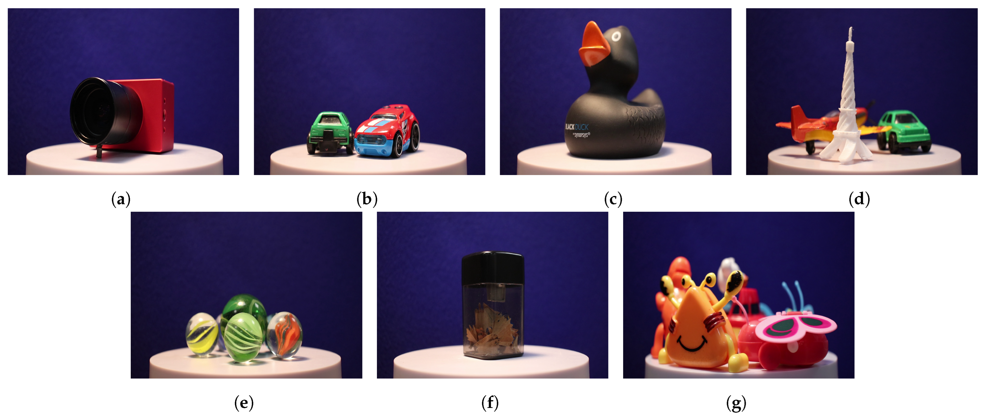
The dataset contains seven distinct sets of objects, some of which consist of multiple objects rather than a single entity. Additionally, two of the contents (‘Marbles’ and ‘Sharpener’) feature semi-translucent objects. Generally, the seven contents were selected with the aim of creating a dataset that is diverse along multiple dimensions (e.g., structural complexity, color variety). Sample views of the captured contents are illustrated in Figure 1.
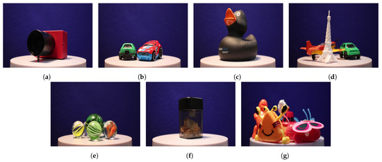
Figure 1.
View samples of the light field dataset: (a) Camera, (b) Cars, (c) Duck, (d) Eiffel, (e) Marbles, (f) Sharpener, and (g) Toys.
Content ‘Camera’ is an actual, functioning, small-scale neuromorphic camera [52]. Content ‘Cars’ consists of two toy cars, one of which is green and black, and the other one is red and light blue. Content ‘Duck’ is a black plastic duck. Content ‘Eiffel’ consists of a small ivory-colored model of the Eiffel tower, as well as a yellow and orange plane and the same green and black toy car from content ‘Cars’. Content ‘Marbles’ is a set of four glass marbles with different patterns and colors. Content ‘Sharpener’ is a conventional pencil sharpener with a transparent container. Content ‘Toys’ consists of four plastic toys, with smooth surfaces and with different variations of the colors red, orange, and purple.
Each content within the dataset was captured in a 53-degree FOV and consists of 70 and 140 views, which—as stated earlier in the paper—correspond to 1.32 and 2.64 views per degree. The dataset was created for the Looking Glass Factory [53] 32-inch, commercially-available light field display, which provides visualization in a 53-degree FOV—which is evidently the reason why the models were captured in a 53-degree FOV.
An alternative solution to capturing the content at both 140 views and 70 views would be to capture 140 views and then use downsampling to achieve the 70 viewss. One way to reduce the angular resolution in such a manner is simply to skip every second view. However, in such a case, either the leftmost or the rightmost view is skipped, resulting in a lower FOV value. The other solution is to utilize an actual downsampling method, yet such may compromise the quality of the content due to their nature—after all, methods such as light field reconstruction, interpolation, and view synthesis are estimations, approximations, and therefore, not perfectly accurate by definition.
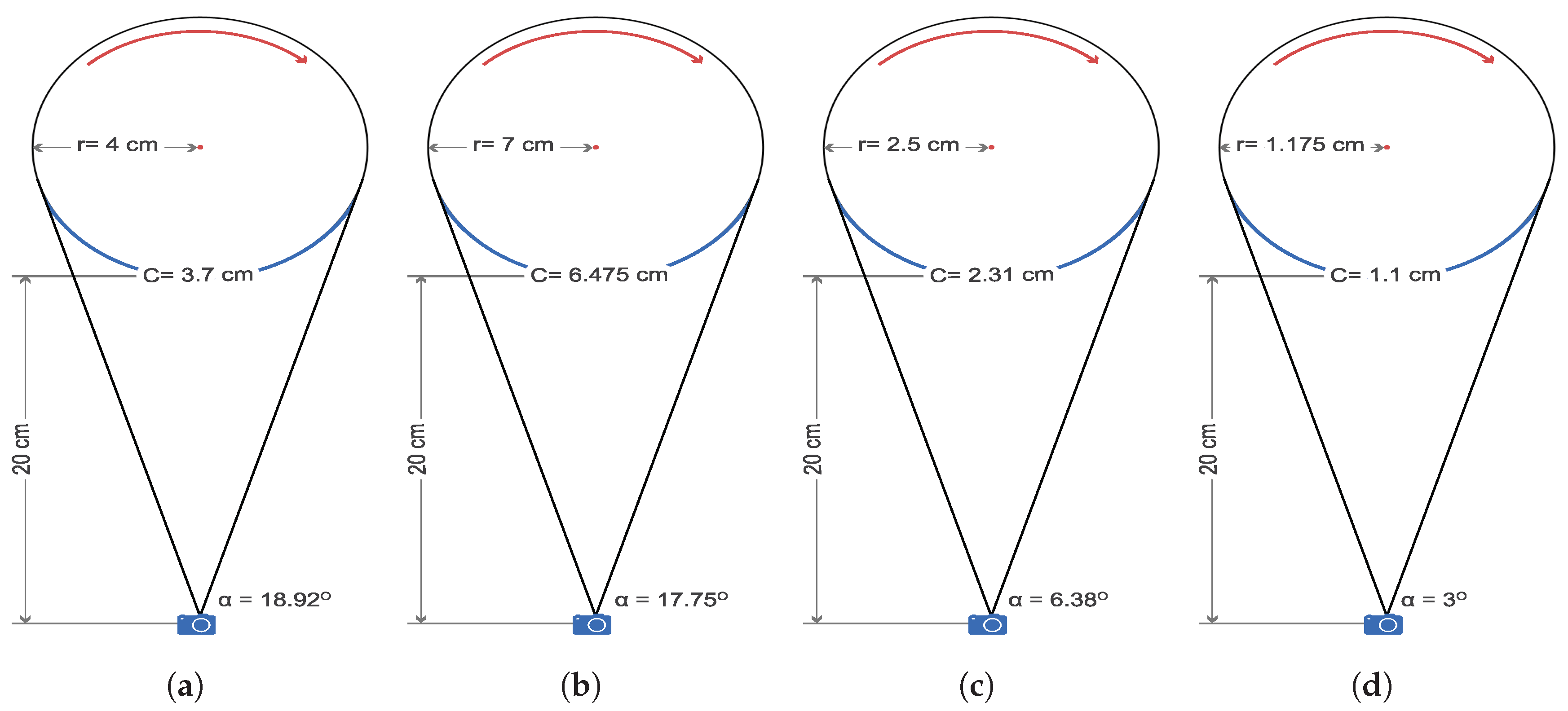
The selected contents were modeled in a circular format to mathematically determine their coverage circumference, and the corresponding camera FOV was measured on the basis of the calculated radius of the objects. This is illustrated in Figure 2.
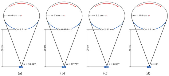
Figure 2.
The FOV of the camera (‘’) and the covered circumference (‘C’) for each content: (a) Camera and Duck, (b) Toys, (c) Cars, Marbles, and Eiffel, and (d) Sharpener.
4. Content Characterization Methodology
Every evaluation in this work is performed on the model variant with higher angular resolution; each input of the analysis consists of 140 views. Additionally, the suffix ‘v’ is appended to every quality metric, denoting that they are sub-metrics based on the available views. In this section, several color measurements are provided, as well as SI, TI, and CF characterizations of light field contents. Since a conventional DSLR camera was used to capture the contents, depth information was not measured initially; it can only be approximated. For example, Ranftl et al. [54] introduced a dense prediction transformer based on neural networks that can be used for such a purpose. Figure 3 shows the depth maps of the view samples of the light field dataset, which were created by using this aforementioned method.
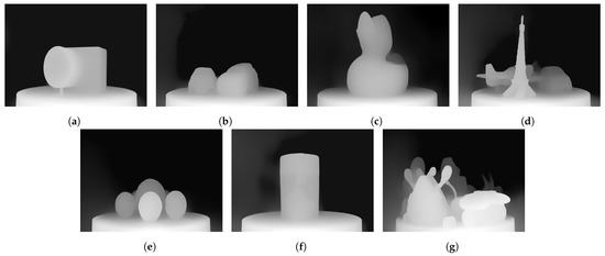
Figure 3.
The depth maps of the view samples of the light field dataset: (a) Camera, (b) Cars, (c) Duck, (d) Eiffel, (e) Marbles, (f) Sharpener, and (g) Toys.
4.1. Color Measurements
The dataset—captured using electronic sensors—employs the RGB color space as its primary representation. The amplitude intensity of each color channel (red, green, and blue) is represented with 8 bits. This leads to values ranging from 0 to 255, providing each channel with the capacity to convey 256 distinct intensity levels.
When considering all three color channels together, they can produce a wide range of colors by combining their respective intensity levels. The total number of unique colors that can be represented in this RGB color space is , resulting in a palette of 16,777,216 distinct colors.
The HSL color space shares a conceptual foundation similar to that of the HSV color space, utilizing a 3D cylindrical coordinate system. However, it distinguishes itself by incorporating the characteristics of two cones within its model. Because of this unique combination of two cones, the HSL color space is often referred to as the “bi-hexcone model” [35]. The equation for transforming from RGB to HSL [34,35] is presented as Equation (1):
where “Max” refers to the maximum value among the red (R), green (G), and blue (B) color channel values in the RGB color model, and “Min” refers to the minimum value.
The conversion from RGB to HSV is described in Equation (2):
where Max = max(R,G,B), Min = min(R,G,B), and the value of A is equal to if H is in radians, and 60 degrees if H is in degrees.
The CIELab color space is designed to closely align with the perceptive capabilities of the human eye. To derive the CIELab color space, a transformation from the RGB to XYZ color space is first performed, followed by a conversion from XYZ to CIELab. Based on the documentation of CIE [55], as well as the works of Schanda [56] and Pardede et al. [35], this conversion process is facilitated using Equations (3)–(5):
The CIE standard Illuminant D65 (6504-degree Kelvin) is provided in Equation (6):
The CIE standard Illuminant D50 (5000-degree Kelvin) is provided in Equation (7):
Equations (1) and (2) are based on the works of Basak et al. [34] and Pardede et al. [35], Equation (3) is also based on the work of Pardede et al. [35], Equation (4) is based on the work of work of Schanda [56], Equation (5) is based on the works of Pardede et al. [35] and Schanda [56], and Equations (6) and (7) are based on the CIE technical report [55].
4.2. , , and Content Characterizations
We propose here three content characterization metrics for light field content, obtained by slightly modifying/adapting three commonly used measures of content complexity (i.e., SI, TI, and colourfulness) to characterize our contents in terms of spatial complexity, inter-view complexity, and colorfulness: , , and , where V refers to “views”. pertains to the distribution and arrangement of visual elements within a static light field scene. normally refers to temporal complexity, in terms of changes in visual content over time, such as motion, movement of objects, or variations in lighting. Here we consider , and we define it as a measure of the changes over the adjacent perspectives. evaluates the intensity and vividness of the views representing the scene.
and are used to calculate the complexity of the light field content, helping to find the correct data rate for real-time light field communication. Higher spatial and temporal values typically require higher data rates to achieve satisfactory quality [57]. We also expect that for light field data, higher and are associated with higher data rates required for compression.
The combination of and allows for a more comprehensive characterization of light field content. For the computation of , the first step is to filter each view out of all available views in the light field content (luminance component) using the Sobel filter. Next, the standard deviation is calculated over the pixels in each Sobel-filtered view. This operation is then repeated for all available views in the light field content, and the maximum value is selected.
To detect horizontal and vertical edges of the luminance component of each view, the kernels of Equations (8) and (9) are applied, respectively:
The mean value is measured in Equation (11):
where P is the number of pixels available in each view. Having the mean value of each Sobel-filtered view in Equation (11), the standard deviation is then calculated in Equation (12) [58]:
The maximum standard deviation value over the views yields , as calculated in Equation (13):
Similar to , plays a critical role in video compression and transmission, as it directly affects the data rate required to represent and transmit a video sequence. Instead of a video containing a series of frames, for the light field contents, we measured the based on the available views within each light field content. To compute , the differences between the corresponding pixels in the luminance component of two successive views are first computed. Then, the standard deviation of the differences is calculated and the maximum value of all views in each light field content is selected as . The initial step in computing the TI value is represented in Equation (14):
where means the pixel intensity difference between the current view , denoted view n, and the previous view , which is view [58].
The standard deviation is computed in Equation (14). The maximum value among all available views of the light field content is selected as the final TI result, as shown in Equation (15):
which is performed for each content within the dataset.
Another method of calculating the complexity of a content or an image is the calculation of the variance of the luminance [57]. We adapt it to our context of light field contents, calculating it for multiple views.
Finally, the value shows the diversity and intensity of the available colors within the images [38], the calculation of which is shown in Equation (16):
where
where represents the standard deviation, and shows the mean value.
5. Data Compression and Objective Quality Assessment Methodology
In order to exploit inter-view redundancy (i.e., the similarities between adjacent perspectives) we compressed the acquired contents using video encoders considering the views as video frames. In particular, the created light field contents—each consisting of 140 views, as stated earlier—are encoded using four different video encoders: AVC [59], HEVC [60], VP9 [61], and AV1 [62], for bit rates ranging from 1 Mbps to 30 Mbps. The fast forward MPEG (ffmpeg) application was used for encoding, but note that the actual bit rate results may not exactly match the specified bit rates due to imperfect rate control in the codecs. More details on this are provided in Section 6.
Following compression, the quality of the impaired contents is assessed by using three quality assessment metrics: , , and , where V—similarly to , , and —refers to “views”. As the objective is to assess the quality of the degraded contents, these metrics calculate the mean of , , and , respectively, over the different views.
Striking a balance between video quality and bandwidth requirements is critical for any compression method, and the added quality metrics will also support further relevant studies, as shown as an example by a recent work [63].
5.1.
One of the methods chosen to assess the quality of the impaired versions of the images/views is PSNR [64], described by Equation (17):
where denotes the highest achievable pixel value within the view, and quantifies the difference between the original and distorted views of the content. is calculated as shown in Equation (18):
where I and K are the original and impaired versions of the view, respectively, and M and N are the dimensions of the view.
The value of varies based on the number of available bits in each single pixel. For instance, if there are 8 bits in each pixel, then the value is equal to , but it starts from zero and ends at 255. Similarly, for 10-bit pixels, the value is equal to , which similarly starts from zero and ends at 1023. This means that there are 1024 different possible values for 10-bit pixels. Therefore, for the first case, the value of is 255, and for 10-bit pixels, the value of is equal to 1023. We consider here:
where V is the number of views.
5.2.
The SSIM [64]—the formula of which is provided in Equation (20)—is a method to measure the similarity between two images. It compares the structural information of an image, such as edges and textures, rather than just comparing the pixel values. This method has been applied in various research studies related to quality assessment [65,66,67,68,69,70,71,72,73].
Unlike —which only measures the difference between two views in terms of their pixel values— is a more comprehensive metric that takes into account the structural information of the views. assesses the perceived quality of views by comparing their luminance, contrast, and structure with that of the reference image. Therefore, is considered a more accurate measure of view quality than , which does not account for the characteristics of the human visual system (HVS).
For example, in the work of Salem et al. [74], both PSNR and SSIM were used to reconstruct the quality assessment metrics.
The main formula is mentioned in Equation (20):
where I and K represent the original and distorted views, while and denote their respective means. Similarly, and refer to the standard deviations of I and K, and represents their covariance. Constants and are included to prevent division by zero. The resulting output varies from 0 to 1, with 1 signifying a perfect similarity between the two images. Similar to the above, we consider here:
where V is the number of views.
6. Content Characterization and Objective Quality Assessment Results
In this section, the aforementioned metrics are utilized to evaluate our novel light field dataset in terms of content complexity and objective quality of the compressed versions of the contents.
6.1. Content Characterization
In this section, we present the analyzed results for color measurements, standard deviation over the available views in each content, and the characterization of spatial, temporal, and colorfulness information.
6.1.1. Color Measurements
Fifteen different result values are provided for each content in the dataset, as shown in Table 1. These results represent the mean values of all pixels in each light field view within the content, followed by the average of all views. This cumulative process generates the single result provided in the table.

Table 1.
The average color measurement values for the contents of the dataset.
The color space range for each component is categorized as below.
HSV:
- Hue describes the color tone, spanning from 0 to 360 degrees;
- Saturation signifies the color’s intensity, with a range of 0% (dull) to 100% (vivid);
- Vivid represents the brightness level, ranging from 0% (completely dark or black) to 100% (full brightness).
HSL:
- Hue defines the color tone and operates within the 0 to 360-degree spectrum;
- Saturation quantifies the color’s intensity, varying from 0% (pale) to 100% (highly saturated);
- This attribute gauges the darkness or lightness of the color and spans from 0% (dark) to 100% (light).
RGB:
- Red Signifies the red color’s intensity, which spans from 0 to 255;
- Green represents the green color’s intensity, which varies from 0 to 255;
- Blue, this parameter quantifies the blue color’s intensity and operates in the 0 to 255 range.
In the CIELab color space, three distinct axes are utilized:
- L measures the transition from darkness to lightness, with values ranging from 0% to 100%,
- –
- Lower values indicate darker colors or shades;
- –
- Higher values correspond to lighter colors or shades.
- a* represents the color axis between green (−128) and red (+127),
- –
- Negative values (−): Suggest a shift towards the green side;
- –
- Positive values (+): Indicate a shift towards the red side.
- b* represents the color axis from blueness (−128) to yellowness (+127),
- –
- Negative values (−): Suggest a shift towards the blue side;
- –
- Positive values (+): Represent a shift towards the yellow side.
6.1.2. Analysis of Standard Deviation across Available Views of the Contents
As highlighted in [57], the variance and standard deviation of the luminance of an image are associated with contrast and hence to its (spatial) complexity for compression; hence, we calculated for the contents in the dataset, the standard deviation of the luminance in each single image/view. The results are shown in Figure 4 in the form of histogram plots, where the x-axis displays the standard deviation values, and the y-axis shows the number of occurrences in all available views for each light field content. The higher the standard deviation values, the higher the (spatial) complexity of the content. We can observe that when the histogram presents spikes, most of the views have a very similar standard deviation/contrast, while “flatter” histograms are associated with a more uniform distribution of standard deviation/contrast values across the views.
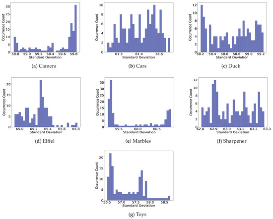
Figure 4.
Histograms of standard deviation measurements for the contents of the dataset. (a–g) Illustrates the results for ‘Camera’, ‘Cars’, ‘Duck’, ‘Eiffel’, ‘Marbles’, ‘Sharpener’, and ‘Toys’, respectively.
6.1.3. Characterization of Spatial, Temporal, and Colorfulness Information
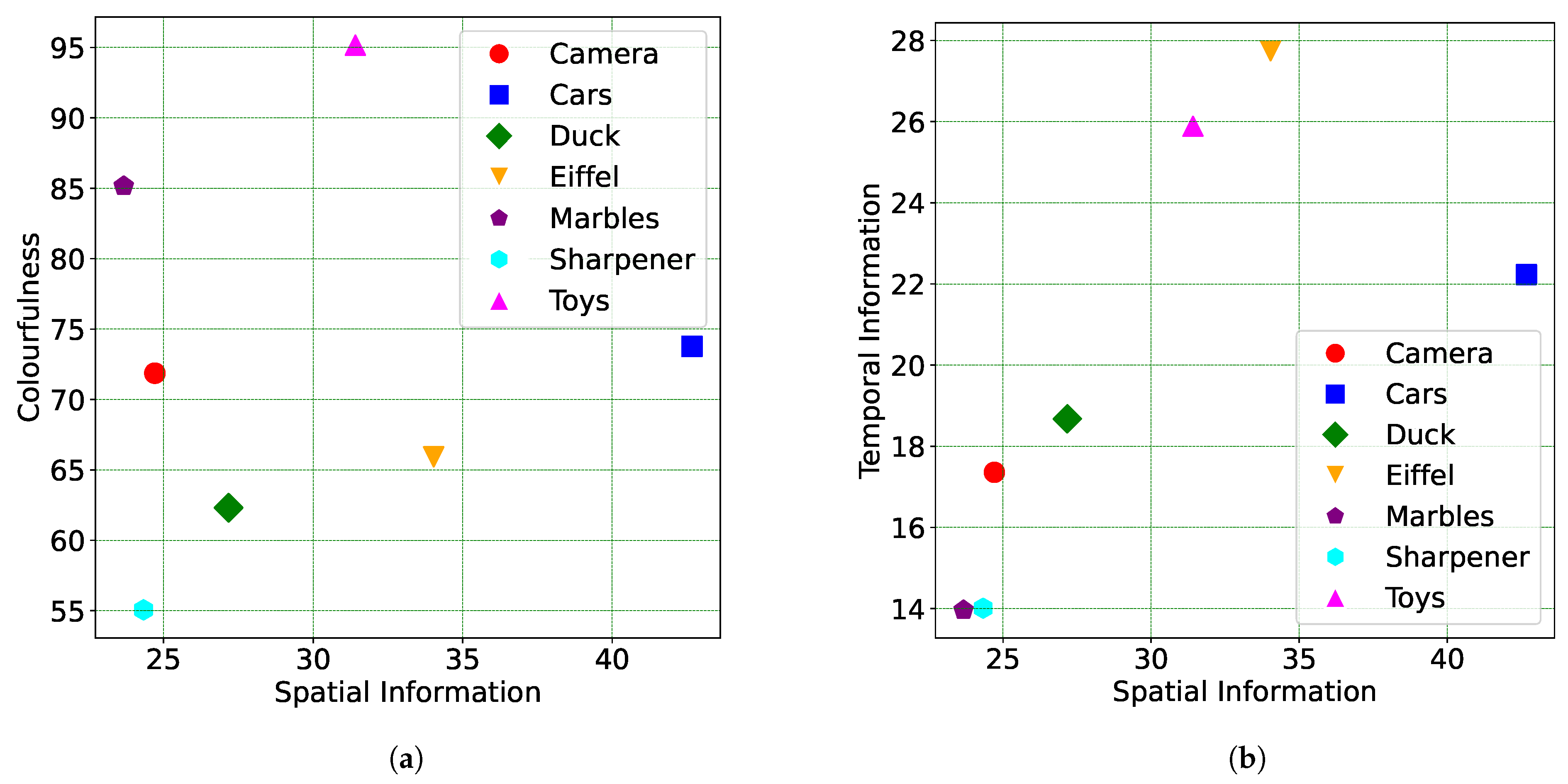
Based on the analysis shown in Figure 5, it is evident that the contents labeled ‘Cars’ and ‘Eiffel’ exhibit higher spatial information across the 140 views. Additionally, in terms of , two of the contents, namely ‘Eiffel’ and ‘Toys’, reached the maximum values among all the contents of the dataset. For the transparent contents, ‘Sharpener’ and ‘Marbles’ exhibit the lowest values in terms of both and across their views. Regarding , content ‘Toys’ demonstrates the highest values. Table 1 presents the results for the different color channels in various color spaces across the 140 views of each content.
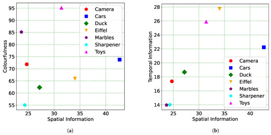
Figure 5.
Content characterization of the acquired scenes. (a) vs. ; (b) vs. .
6.2. Data Compression
As highlighted before, the actual datarates are often different from the values set for encoding, due to inaccuracies in the rate-control algorithms adopted in the codecs. The results of the actual bitrate values obtained are provided in Table 2 and Table 3. The first column of the table reports the bitrate value sets in the codecs (in Mbps). We refer to bitrates rather than file size for the scene since we consider the views of a static scene as the frames of a video for the encoding process. Since the encoding was performed assuming 30 fps, 1 Mbps means that, on average, each view is represented with 33 kbits hence 140 views with 4.67 Mbits or 583 kB, while 30 Mbps correspond to a file size of 17.5 MB. The other columns report the actual values obtained with different codecs for the different contents.
Table 2.
The actual practical results (in Mbps) of the encoders for contents Camera, Cars, Duck, and Eiffel.
Table 3.
The actual practical results (in Mbps) of the encoders for contents Marbles, Sharpener, and Toys.
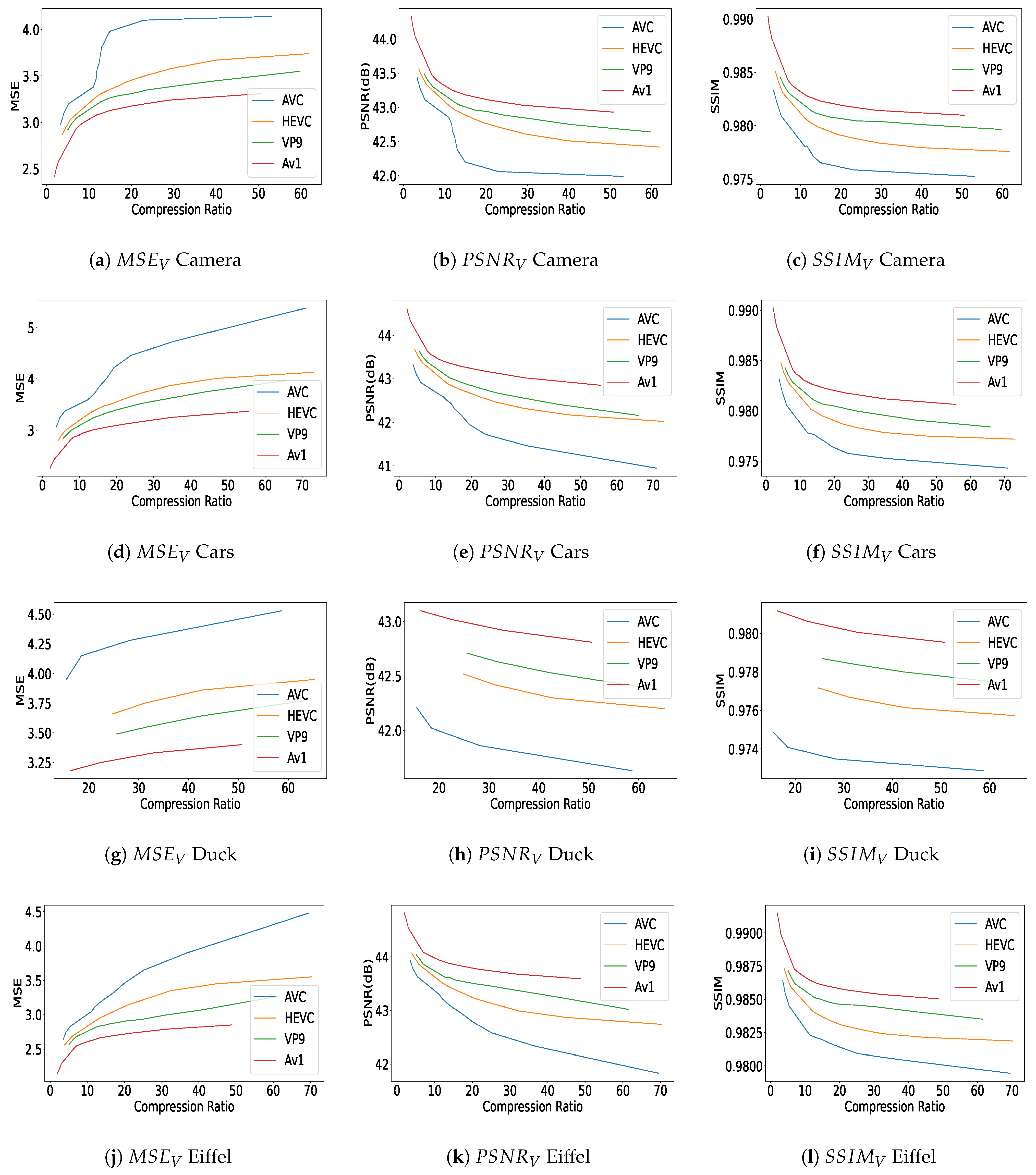
The quality results—as depicted in Figure 6 and Figure 7—clearly demonstrate how the inconsistency between the applied bit rates and the actual values—all listed in Table 2 and Table 3—affects the plot lengths, causing them to be unequal.
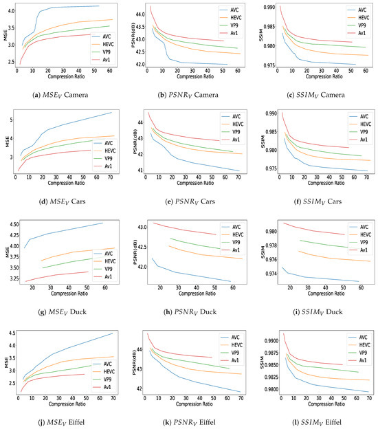
Figure 6.
Quality assessments for different compression ratios were performed using various quality metrics and each row of the plots presents the results for one content, including measurements in (a,d,g,j); measurements in (b,e,h,k); and evaluations in (c,f,i,l). These assessments were conducted on content categorized as ‘Camera’, ‘Cars’, ‘Duck’, and ‘Eiffel’, each representing different types of visual data. In each graph, distinct curves represent the results obtained from different codecs.
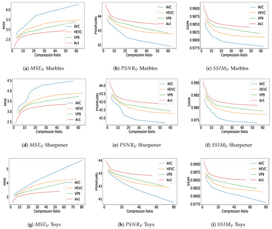
Figure 7.
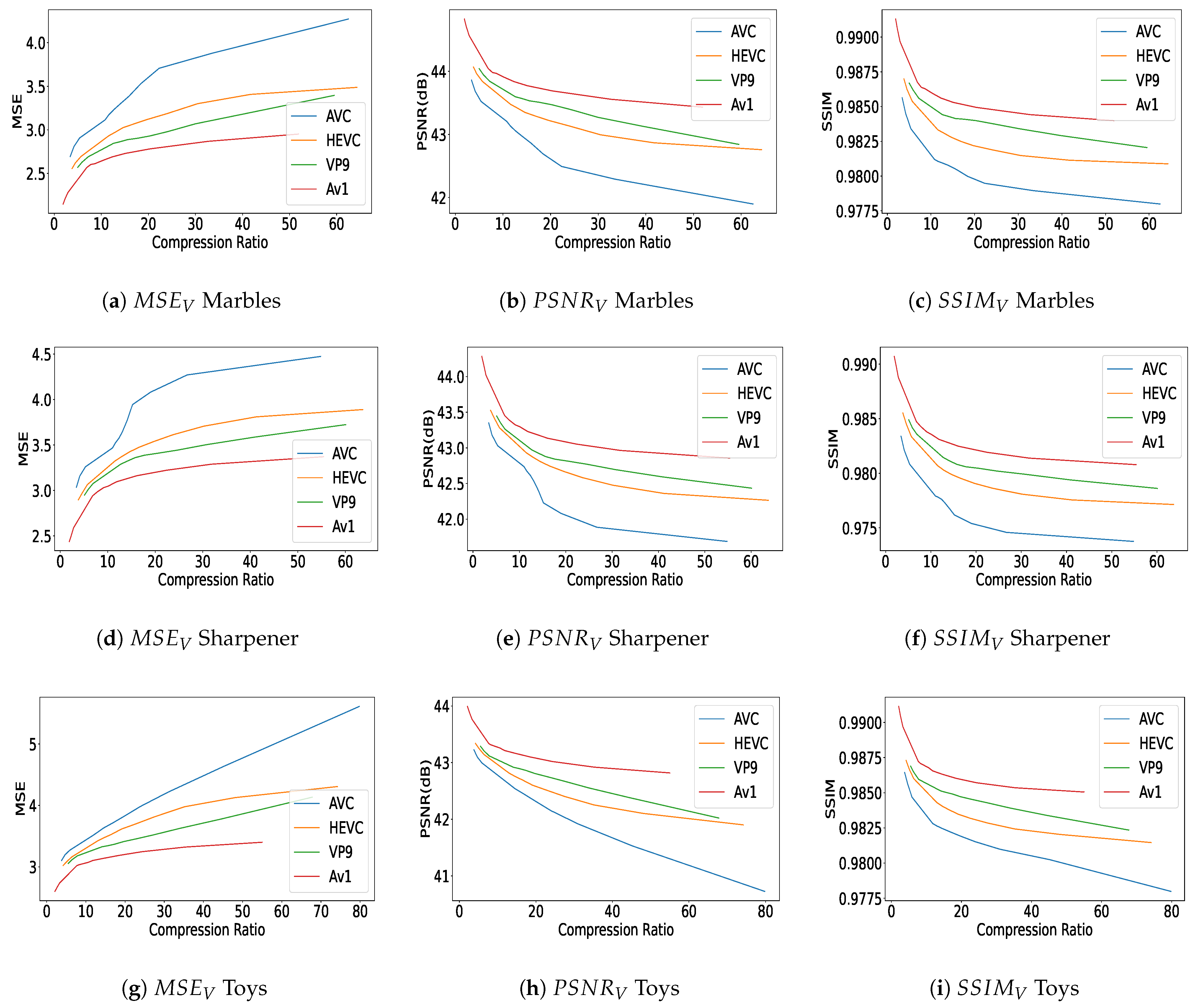
Objective quality assessments via , , and versus different compression ratios. (a–c) quality-metric plots for ‘Marbles’, (d–f) show quality metrics for ‘Sharpener’, and (g–i) present results for ‘Toys’ content, all evaluated based on different compression ratios.
6.3. Objective Quality Assessment Results
Following the characterization analysis of the contents mentioned above and compression, the quality of the compressed versions is objectively assessed.
To accomplish this, all contents are initially encoded with varying bit rate values and by different encoders, including AVC, HEVC, VP9, and AV1. Subsequently, the quality of the impaired encoded contents is evaluated in relation to the original contents (“full-reference” quality assessment).
Figure 6 and Figure 7 report the objective quality results in terms of , , and versus compression ratio, for the different contents (‘Camera’, ‘Cars’, ‘Duck’, ‘Eiffel’ in Figure 6 and ‘Marbles’, ‘Sharpener’, and ‘Toys’ in Figure 7). We can observe that AV1 performs the best in terms of quality assessment for both / and . Following AV1, VP9 is the second best encoder, followed by HEVC and then AVC, which shows the lowest performance for our dataset. Armipour et al. [75] and Hajihashemi et al. [76] used the same evaluation methods for their light field contents, with some differences in the performance of certain codecs. Quality values follow the order of highest to lowest for AV1, VP9, HEVC, and AVC, respectively. It is notable that all the mentioned encoders are applied to all 140 views within each content of the light field dataset, followed by the application of the attributed quality metrics. We can also observe that quality values span a wider range for some of the contents (e.g., ‘Cars’ and ‘Toys’) than for others (e.g., ‘Duck’). Since the texture of the objects is relatively simple and the background is quite uniform, high compression ratios are achieved in general, while a very high quality is kept.
7. Conclusions
In conclusion, this paper presented a novel light field dataset captured using the Canon 77D DSLR camera, with the aim to support future research on displays with a 53 degrees viewing cone, such as the 32-inch Looking Glass Factory light field display, particularly in the field of subjective quality assessment. Various measures for content characterization were calculated for the contents in this dataset. Moreover, different encoders were applied to the contents in the proposed dataset, covering all 140 available views of each content, with varying compression ratios. Quality scores of the compressed versions are also provided, calculated via commonly used objective quality metrics.
In future work, the introduced light field contents shall undergo subjective evaluation on the aforementioned light field display, with a particular focus on assessing the transparency effects during display. We also plan to expand the dataset, for instance, with further codecs, including versatile video coding (VVC) [77].
Author Contributions
Conceptualization, K.J., M.G.M. and P.A.K.; methodology, K.J., M.G.M. and P.A.K.; validation, K.J.; investigation, K.J.; resources, K.J. and M.G.M.; writing—original draft preparation, K.J., M.G.M. and P.A.K.; writing—review and editing, K.J., M.G.M. and P.A.K.; visualization, K.J.; supervision, M.G.M. and P.A.K.; project administration, M.G.M. All authors have read and agreed to the published version of the manuscript.
Funding
This research received no external funding.
Data Availability Statement
The dataset is publicly available via the following link: https://bit.ly/KULF-TT53, accessed on 20 October 2023.
Acknowledgments
The authors would like to thank Edris Shafiee for his support.
Conflicts of Interest
The authors declare no conflict of interest.
Abbreviations
The following abbreviations are used in this manuscript:
| AV1 | AOMedia Video 1 |
| AVC | Advanced Video Coding |
| CF | Colorfulness |
| CIE | Commission Internationale de l’Eclairage (International Commission on Illumination) |
| CNN | Convolutional Neural Network |
| DSLR | Digital Single-Lens Reflex |
| FP | Full Parallax |
| fps | frames per second |
| HEVC | High Efficiency Video Coding |
| HOP | Horizontal-Only Parallax |
| HSV | Hue-Saturation-Value |
| HSL | Hue-Saturation-Lightness |
| KPI | Key Performance Indicator |
| LCD | Liquid-Crystal Display |
| LED | Light-Emitting Diode |
| Mbps | Megabits per second |
| MLR | Multiple Linear Regression |
| MSE | Mean Square Error |
| PSNR | Peak Signal-to-Noise Ratio |
| RGB | Red, Green, Blue |
| RGB-D | Red, Green, Blue plus Depth |
| SI | Spatial Information |
| SMV | Super MultiView |
| SSIM | Structural Similarity Index |
| TI | Temporal Information |
| VGA | Video Graphics Array |
| VVA | Valid Viewing Area |
| VVC | Versatile Video Coding |
| VP9 | Video Codec 9 |
References
- IEEE P3333.1.4-2022; Recommended Practice for the Quality Assessment of Light Field Imaging. IEEE Standards Association: Piscataway, NJ, USA, 2023.
- International Committee for Display Metrology (ICDM); Society for Information Display (SID). Information Display Measurements Standard (IDMS) v1.2. 2023. Available online: https://www.sid.org/Standards/ICDM (accessed on 29 October 2023).
- Tamboli, R.R.; Appina, B.; Channappayya, S.; Jana, S. Super-multiview content with high angular resolution: 3D quality assessment on horizontal-parallax lightfield display. Signal Process. Image Commun. 2016, 47, 42–55. [Google Scholar] [CrossRef]
- Recio, R.; Carballeira, P.; Gutiérrez, J.; García, N. Subjective assessment of super multiview video with coding artifacts. IEEE Signal Process. Lett. 2017, 24, 868–871. [Google Scholar] [CrossRef]
- Tamboli, R.R.; Appina, B.; Channappayya, S.S.; Jana, S. Achieving high angular resolution via view synthesis: Quality assessment of 3D content on super multiview lightfield display. In Proceedings of the 2017 International Conference on 3D Immersion (IC3D), Brussels, Belgium, 11–12 December 2017; pp. 1–8. [Google Scholar]
- Peng, W.; Sang, X.; Xing, S. High-efficiency generating of photorealistic super-multiview image for glasses-free three-dimensional display based on distributed rendering. In Proceedings of the Optoelectronic Imaging and Multimedia Technology V, SPIE, Beijing, China, 11–12 October 2018; Volume 10817, pp. 244–254. [Google Scholar]
- Xing, S.; Sang, X.; Cao, L.; Guan, Y.; Li, Y. A real-time super multiview rendering pipeline for wide viewing-angle and high-resolution 3D displays based on a hybrid rendering technique. IEEE Access 2020, 8, 85750–85759. [Google Scholar] [CrossRef]
- Kara, P.A.; Tamboli, R.R.; Doronin, O.; Cserkaszky, A.; Barsi, A.; Nagy, Z.; Martini, M.G.; Simon, A. The key performance indicators of projection-based light field visualization. J. Inf. Disp. 2019, 20, 81–93. [Google Scholar] [CrossRef]
- Georgiev, T.G.; Zheng, K.C.; Curless, B.; Salesin, D.; Nayar, S.K.; Intwala, C. Spatio-Angular Resolution Tradeoffs in Integral Photography. Render. Tech. 2006, 2006, 21. [Google Scholar]
- Kovács, P.T.; Bregović, R.; Boev, A.; Barsi, A.; Gotchev, A. Quantifying spatial and angular resolution of light-field 3-D displays. IEEE J. Sel. Top. Signal Process. 2017, 11, 1213–1222. [Google Scholar] [CrossRef]
- Kara, P.A.; Cserkaszky, A.; Barsi, A.; Papp, T.; Martini, M.G.; Bokor, L. The interdependence of spatial and angular resolution in the quality of experience of light field visualization. In Proceedings of the 2017 International Conference on 3D Immersion (IC3D), Brussels, Belgium, 11–12 December 2017; pp. 1–8. [Google Scholar]
- Tamboli, R.R.; Appina, B.; Kara, P.A.; Martini, M.G.; Channappayya, S.S.; Jana, S. Effect of primitive features of content on perceived quality of light field visualization. In Proceedings of the 2018 Tenth International Conference on Quality of Multimedia Experience (QoMEX), Cagliari, Italy, 29 May–1 June 2018; pp. 1–3. [Google Scholar]
- Shi, L.; Zhao, S.; Zhou, W.; Chen, Z. Perceptual evaluation of light field image. In Proceedings of the 2018 25th IEEE International Conference on Image Processing (ICIP), Athens, Greece, 7–10 October 2018; pp. 41–45. [Google Scholar]
- Zhou, W.; Shi, L.; Chen, Z.; Zhang, J. Tensor oriented no-reference light field image quality assessment. IEEE Trans. Image Process. 2020, 29, 4070–4084. [Google Scholar] [CrossRef] [PubMed]
- Adhikarla, V.K.; Vinkler, M.; Sumin, D.; Mantiuk, R.K.; Myszkowski, K.; Seidel, H.P.; Didyk, P. Towards a quality metric for dense light fields. In Proceedings of the IEEE Conference on Computer Vision and Pattern Recognition, Honolulu, HI, USA, 21–26 July 2017; pp. 58–67. [Google Scholar]
- Shi, L.; Zhou, W.; Chen, Z.; Zhang, J. No-reference light field image quality assessment based on spatial-angular measurement. IEEE Trans. Circuits Syst. Video Technol. 2019, 30, 4114–4128. [Google Scholar] [CrossRef]
- Viola, I.; Ebrahimi, T. VALID: Visual quality assessment for light field images dataset. In Proceedings of the 2018 Tenth International Conference on Quality of Multimedia Experience (QoMEX), IEEE, Cagliari, Italy, 29 May–1 June 2018; pp. 1–3. [Google Scholar]
- Luo, Z.; Zhou, W.; Shi, L.; Chen, Z. No-reference light field image quality assessment based on micro-lens image. In Proceedings of the 2019 Picture Coding Symposium (PCS), IEEE, Ningbo, China, 12–15 November 2019; pp. 1–5. [Google Scholar]
- Paudyal, P.; Olsson, R.; Sjöström, M.; Battisti, F.; Carli, M. SMART: A Light Field Image Quality Dataset. In Proceedings of the 7th International Conference on Multimedia Systems, MMSys’16, New York, NY, USA, 10–13 May 2016. [Google Scholar]
- Rerabek, M.; Yuan, L.; Authier, L.A.; Ebrahimi, T. [ISO/IEC JTC 1/SC 29/WG1 Contribution] EPFL Light-Field Image Dataset. Technical Report. 2015. Available online: https://infoscience.epfl.ch/record/209930?ln=en (accessed on 29 October 2023).
- Rerabek, M.; Ebrahimi, T. New light field image dataset. In Proceedings of the 8th International Conference on Quality of Multimedia Experience (QoMEX), Lisbon, Portugal, 6–8 June 2016. [Google Scholar]
- Wang, T.C.; Zhu, J.Y.; Hiroaki, E.; Chandraker, M.; Efros, A.A.; Ramamoorthi, R. A 4D light-field dataset and CNN architectures for material recognition. In Proceedings of the Computer Vision—ECCV 2016: 14th European Conference, Amsterdam, The Netherlands, 11–4 October 2016; Proceedings, Part III 14. Springer: Cham, Switzerland, 2016; pp. 121–138. [Google Scholar]
- Shan, L.; An, P.; Liu, D.; Ma, R. Subjective evaluation of light field images for quality assessment database. In Proceedings of the Digital TV and Wireless Multimedia Communication: 14th International Forum, IFTC 2017, Shanghai, China, 8–9 November 2017; Revised Selected Papers 14. Springer: Singapore, 2018; pp. 267–276. [Google Scholar]
- Tamboli, R.R.; Reddy, M.S.; Kara, P.A.; Martini, M.G.; Channappayya, S.S.; Jana, S. A high-angular-resolution turntable data-set for experiments on light field visualization quality. In Proceedings of the 2018 Tenth International Conference on Quality of Multimedia Experience (QoMEX), Cagliari, Italy, 29 May–1 June 2018; pp. 1–3. [Google Scholar]
- Shekhar, S.; Kunz Beigpour, S.; Ziegler, M.; Chwesiuk, M.; Paleń, D.; Myszkowski, K.; Keinert, J.; Mantiuk, R.; Didyk, P. Light-field intrinsic dataset. In Proceedings of the British Machine Vision Conference 2018 (BMVC), British Machine Vision Association, Newcastle upon Tyne, UK, 3–6 September 2018. [Google Scholar]
- Zakeri, F.S.; Durmush, A.; Ziegler, M.; Bätz, M.; Keinert, J. Non-planar inside-out dense light-field dataset and reconstruction pipeline. In Proceedings of the 2019 IEEE International Conference on Image Processing (ICIP), Taipei, Taiwan, 22–25 September 2019; pp. 1059–1063. [Google Scholar]
- Wanner, S.; Meister, S.; Goldluecke, B. Datasets and benchmarks for densely sampled 4D light fields. In Proceedings of the Vision, Modeling, and Visualization (VMV), Lugano, Switzerland, 11–13 September 2013; Volume 13, pp. 225–226. [Google Scholar]
- Wu, Y.; Liu, S.; Sun, C.; Zeng, B. Light-field raw data synthesis from RGB-D images: Pushing to the extreme. IEEE Access 2020, 8, 33391–33405. [Google Scholar] [CrossRef]
- Guillo, L.; Jiang, X.; Lafruit, G.; Guillemot, C. Light Field Video Dataset Captured by a r8 Raytrix Camera (with Disparity Maps); International Organisation for Standardisation ISO/IEC JTC1/SC29/WG1 & WG11; International Organisation for Standardisation: Geneva, Switzerland, 2018. [Google Scholar]
- Vaish, V.; Adams, A. The (new) stanford light field archive. Comput. Graph. Lab. Stanf. Univ. 2008, 6, 3. [Google Scholar]
- Yu, L.; Ma, Y.; Hong, S.; Chen, K. Review of Light Field Image Super-Resolution. Electronics 2022, 11, 1904. [Google Scholar] [CrossRef]
- Shafiee, E.; Martini, M.G. Datasets for the quality assessment of light field imaging: Comparison and future directions. IEEE Access 2023, 11, 15014–15029. [Google Scholar] [CrossRef]
- Bora, D.J.; Gupta, A.K.; Khan, F.A. Comparing the performance of L*A*B* and HSV color spaces with respect to color image segmentation. arXiv 2015, arXiv:1506.01472. [Google Scholar]
- Basak, J.K.; Madhavi, B.G.K.; Paudel, B.; Kim, N.E.; Kim, H.T. Prediction of total soluble solids and pH of strawberry fruits using RGB, HSV and HSL colour spaces and machine learning models. Foods 2022, 11, 2086. [Google Scholar] [CrossRef] [PubMed]
- Pardede, J.; Husada, M.G.; Hermana, A.N.; Rumapea, S.A. Fruit Ripeness Based on RGB, HSV, HSL, L*a*b* Color Feature Using SVM. In Proceedings of the 2019 International Conference of Computer Science and Information Technology (ICoSNIKOM), Medan, Indonesia, 28–29 November 2019; pp. 1–5. [Google Scholar]
- Ravishankar, J.; Sharma, M.; Gopalakrishnan, P. A Flexible Coding Scheme Based on Block Krylov Subspace Approximation for Light Field Displays with Stacked Multiplicative Layers. Sensors 2021, 21, 4574. [Google Scholar] [CrossRef]
- Indrabayu, I.; Arifin, N.; Areni, I.S. Strawberry ripeness classification system based on skin tone color using multi-class support vector machine. In Proceedings of the 2019 International Conference on Information and Communications Technology (ICOIACT), Yogyakarta, Indonesia, 24–25 July 2019; pp. 191–195. [Google Scholar]
- de Faria, S.M.; Filipe, J.N.; Pereira, P.M.; Tavora, L.M.; Assuncao, P.A.; Santos, M.O.; Fonseca-Pinto, R.; Santiago, F.; Dominguez, V.; Henrique, M. Light field image dataset of skin lesions. In Proceedings of the 2019 41st Annual International Conference of the IEEE Engineering in Medicine and Biology Society (EMBC), Berlin, Germany, 23–27 July 2019; pp. 3905–3908. [Google Scholar]
- Barman, N.; Khan, N.; Martini, M.G. Analysis of spatial and temporal information variation for 10-bit and 8-bit video sequences. In Proceedings of the 2019 IEEE 24th International Workshop on Computer Aided Modeling and Design of Communication Links and Networks (CAMAD), Limassol, Cyprus, 11–13 September 2019; pp. 1–6. [Google Scholar]
- Amirpour, H.; Pinheiro, A.M.; Pereira, M.; Ghanbari, M. Reliability of the most common objective metrics for light field quality assessment. In Proceedings of the ICASSP 2019—2019 IEEE International Conference on Acoustics, Speech and Signal Processing (ICASSP), Brighton, UK, 12–17 May 2019; pp. 2402–2406. [Google Scholar]
- PhiCong, H.; Perry, S.; Cheng, E.; HoangVan, X. Objective quality assessment metrics for light field image based on textural features. Electronics 2022, 11, 759. [Google Scholar] [CrossRef]
- Perra, C.; Astola, P.; Da Silva, E.A.; Khanmohammad, H.; Pagliari, C.; Schelkens, P.; Tabus, I. Performance analysis of JPEG Pleno light field coding. In Proceedings of the Applications of Digital Image Processing XLII. SPIE, San Diego, CA, USA, 11–15 August 2019; Volume 11137, pp. 402–413. [Google Scholar]
- Wang, Y.; Wang, L.; Yang, J.; An, W.; Yu, J.; Guo, Y. Spatial-angular interaction for light field image super-resolution. In Proceedings of the Computer Vision—ECCV 2020: 16th European Conference, Glasgow, UK, 23–28 August 2020; Proceedings, Part XXIII 16. Springer: Cham, Switzerland, 2020; pp. 290–308. [Google Scholar]
- Jin, K.; Yang, A.; Wei, Z.; Guo, S.; Gao, M.; Zhou, X. Distgepit: Enhanced disparity learning for light field image super-resolution. In Proceedings of the IEEE/CVF Conference on Computer Vision and Pattern Recognition, Vancouver, BC, Canada, 17–24 June 2023; pp. 1373–1383. [Google Scholar]
- Xiao, Z.; Gao, R.; Liu, Y.; Zhang, Y.; Xiong, Z. Toward Real-World Light Field Super-Resolution. In Proceedings of the IEEE/CVF Conference on Computer Vision and Pattern Recognition, Vancouver, BC, Canada, 17–24 June 2023; pp. 3407–3417. [Google Scholar]
- Yu, H.; Julin, J.; Milacski, Z.A.; Niinuma, K.; Jeni, L.A. DyLiN: Making Light Field Networks Dynamic. In Proceedings of the IEEE/CVF Conference on Computer Vision and Pattern Recognition, Vancouver, BC, Canada, 17–24 June 2023; pp. 12397–12406. [Google Scholar]
- Kara, P.A.; Tamboli, R.R.; Shafiee, E.; Martini, M.G.; Simon, A.; Guindy, M. Beyond perceptual thresholds and personal preference: Towards novel research questions and methodologies of quality of experience studies on light field visualization. Electronics 2022, 11, 953. [Google Scholar] [CrossRef]
- Darukumalli, S.; Kara, P.A.; Barsi, A.; Martini, M.G.; Balogh, T.; Chehaibi, A. Performance comparison of subjective assessment methodologies for light field displays. In Proceedings of the 2016 IEEE International Symposium on Signal Processing and Information Technology (ISSPIT), Limassol, Cyprus, 12–14 December 2016; pp. 28–33. [Google Scholar]
- Guindy, M.; Barsi, A.; Kara, P.A.; Adhikarla, V.K.; Balogh, T.; Simon, A. Camera animation for immersive light field imaging. Electronics 2022, 11, 2689. [Google Scholar] [CrossRef]
- Simon, A.; Kara, P.A.; Guindy, M.; Qiu, X.; Szy, L.; Balogh, T. One step closer to a better experience: Analysis of the suitable viewing distance ranges of light field visualization usage contexts for observers with reduced visual capabilities. In Proceedings of the Novel Optical Systems, Methods, and Applications XXV, SPIE, San Diego, CA, USA, 21–26 August 2022; Volume 12216, pp. 133–143. [Google Scholar]
- Canon. Canon EOS 77D DSLR Camera. Available online: https://www.canon.co.uk/cameras/eos-77d/ (accessed on 29 October 2023).
- IniVation Neuromorphic VISION Systems. Available online: https://inivation.com/ (accessed on 29 October 2023).
- Looking Glass Factory. Looking Glass 32" Immersive 3D Display. Available online: https://lookingglassfactory.com/looking-glass-32 (accessed on 29 October 2023).
- Ranftl, R.; Bochkovskiy, A.; Koltun, V. Vision Transformers for Dense Prediction. In Proceedings of the 2021 IEEE/CVF International Conference on Computer Vision (ICCV), Montreal, QC, Canada, 10–17 October 2021; pp. 12179–12188. [Google Scholar]
- Commission Internationale de l’Éclairage. Cie 1976 L*A*B* Colour Space; Technical Report CIE 15:2004; Commission Internationale de l’Éclairage: Vienna, Austria, 1976. [Google Scholar]
- Schanda, J. Colorimetry: Understanding the CIE System; John Wiley and Sons: Hoboken, NJ, USA, 2007; p. 61. ISBN 978-0-470-04904-4. [Google Scholar]
- Al-Juboori, S.; Martini, M.G. Content Characterization for Live Video Compression Optimization. TechRxiv 2022, in press. [Google Scholar]
- Zhang, R.; Regunathan, S.L.; Rose, K. Video coding with optimal inter/intra-mode switching for packet loss resilience. IEEE J. Sel. Areas Commun. 2000, 18, 966–976. [Google Scholar] [CrossRef]
- ITU-T Recommendation H.264: Advanced Video Coding for Generic Audiovisual Services. 2003. Available online: https://www.itu.int/rec/T-REC-H.264 (accessed on 29 October 2023).
- ITU-T Recommendation H.265: High Efficiency Video Coding. 2013. Available online: https://www.itu.int/rec/T-REC-H.265 (accessed on 29 October 2023).
- Internet Engineering Task Force (IETF) RFC 7741, WebM Project: VP9 Bitstream Specification. 2016. Available online: https://www.webmproject.org/vp9/ (accessed on 29 October 2023).
- Alliance for Open Media: AV1 Bitstream and Decoding Process Specification. 2021. Available online: https://aomedia.org/av1-features/ (accessed on 29 October 2023).
- Klink, J. A method of codec comparison and selection for good quality video transmission over limited-bandwidth networks. Sensors 2021, 21, 4589. [Google Scholar] [CrossRef] [PubMed]
- Wang, Z.; Bovik, A.C.; Sheikh, H.R.; Simoncelli, E.P. Image quality assessment: From error visibility to structural similarity. IEEE Trans. Image Process. 2004, 13, 600–612. [Google Scholar] [CrossRef] [PubMed]
- Hariharan, H.P.; Lange, T.; Herfet, T. Low complexity light field compression based on pseudo-temporal circular sequencing. In Proceedings of the 2017 IEEE International Symposium on Broadband Multimedia Systems and Broadcasting (BMSB), Cagliari, Italy, 7–9 June 2017; pp. 1–5. [Google Scholar]
- Zhang, S.; Lin, Y.; Sheng, H. Residual networks for light field image super-resolution. In Proceedings of the IEEE/CVF Conference on Computer Vision and Pattern Recognition, Long Beach, CA, USA, 15–20 June 2019; pp. 11046–11055. [Google Scholar]
- Mehajabin, N.; Pourazad, M.; Nasiopoulos, P. SSIM assisted Pseudo-sequence-based prediction structure for light field video compression. In Proceedings of the 2020 IEEE International Conference on Consumer Electronics (ICCE), Las Vegas, NV, USA, 4–6 January 2020; pp. 1–2. [Google Scholar]
- Sakamoto, T.; Kodama, K.; Hamamoto, T. A study on efficient compression of multi-focus images for dense light-field reconstruction. In Proceedings of the 2012 Visual Communications and Image Processing, San Diego, CA, USA, 27–30 November 2012; pp. 1–6. [Google Scholar]
- Omidi, P.; Safari, M.; Thibault, S.; Wong, H.M. Optimization of 3D light field display by neural network based image deconvolution algorithm. In Proceedings of the Advances in Display Technologies XIII, SPIE, San Francisco, CA, USA, 28 January–3 February 2023; Volume 12443, pp. 128–135. [Google Scholar]
- Gao, S.; Qu, G.; Sjöström, M.; Liu, Y. A TV regularisation sparse light field reconstruction model based on guided-filtering. Signal Process. Image Commun. 2022, 109, 116852. [Google Scholar] [CrossRef]
- Çetinkaya, E.; Amirpour, H.; Timmerer, C. LFC-SASR: Light Field Coding Using Spatial and Angular Super-Resolution. In Proceedings of the 2022 IEEE International Conference on Multimedia and Expo Workshops (ICMEW), Taipei City, Taiwan, 18–22 July 2022; pp. 1–6. [Google Scholar]
- Zhong, L.; Zong, B.; Wang, Q.; Yu, J.; Zhou, W. Implicit Epipolar Geometric Function Based Light Field Continuous Angular Representation. In Proceedings of the IEEE/CVF Conference on Computer Vision and Pattern Recognition, Vancouver, BC, Canada, 17–24 June 2023; pp. 3462–3471. [Google Scholar]
- Yang, C.C.; Chen, Y.C.; Chen, S.L.; Chen, H.H. Disparity-guided light field video synthesis with temporal consistency. In Proceedings of the 2022 IEEE 5th International Conference on Multimedia Information Processing and Retrieval (MIPR), Virtual. 2–4 August 2022; pp. 178–183. [Google Scholar]
- Salem, A.; Ibrahem, H.; Kang, H.S. RCA-LF: Dense Light Field Reconstruction Using Residual Channel Attention Networks. Sensors 2022, 22, 5254. [Google Scholar] [CrossRef]
- Amirpour, H.; Pinheiro, A.M.; Fonseca, E.; Ghanbari, M.; Pereira, M. Quality evaluation of holographic images coded with standard codecs. IEEE Trans. Multimed. 2021, 24, 3256–3264. [Google Scholar] [CrossRef]
- Hajihashemi, V.; Gharahbagh, A.A.; Bastanfard, A.; Oliveira, H.S.; Almeida, G.; Ma, Z.; Tavares, J.M.R. A Hierarchical modified AV1 Codec for Compression Cartesian form of Holograms in Holo and Object planes. Multimed. Tools Appl. 2023, 82, 8303–8321. [Google Scholar] [CrossRef]
- Bross, B.; Wang, Y.K.; Ye, Y.; Liu, S.; Chen, J.; Sullivan, G.J.; Ohm, J.R. Overview of the versatile video coding (VVC) standard and its applications. IEEE Trans. Circuits Syst. Video Technol. 2021, 31, 3736–3764. [Google Scholar] [CrossRef]


Disclaimer/Publisher’s Note: The statements, opinions and data contained in all publications are solely those of the individual author(s) and contributor(s) and not of MDPI and/or the editor(s). MDPI and/or the editor(s) disclaim responsibility for any injury to people or property resulting from any ideas, methods, instructions or products referred to in the content. |
© 2023 by the authors. Licensee MDPI, Basel, Switzerland. This article is an open access article distributed under the terms and conditions of the Creative Commons Attribution (CC BY) license (https://creativecommons.org/licenses/by/4.0/).