Abstract
Sustaining global food security amid a growing world population demands advanced breeding methods. Phenotyping, which observes and measures physical traits, is a vital component of agricultural research. However, its labor-intensive nature has long hindered progress. In response, we present an efficient phenotyping platform tailored specifically for cucumbers, harnessing smartphone cameras for both cost-effectiveness and accessibility. We employ state-of-the-art computer vision models for zero-shot cucumber phenotyping and introduce a B-spline curve as a medial axis to enhance measurement accuracy. Our proposed method excels in predicting sample lengths, achieving an impressive mean absolute percentage error (MAPE) of 2.20%, without the need for extensive data labeling or model training.
1. Introduction
Sustaining global food security in the face of a growing world population remains a persistent challenge. Meeting this challenge necessitates the continuous development of advanced breeding methods. Modern genomics-assisted breeding (GAB) represents a pivotal approach in this context, involving the intricate analysis of a plant’s genetic makeup to identify specific genes or markers linked to desirable traits. This genetic insight empowers breeders to make informed choices when selecting parent plants for crossbreeding, ultimately yielding new plant breeds that inherit the desired traits. Central to the success of GAB is phenotyping—a vital component that complements genetic analysis. Phenotyping encompasses the detailed observation and measurement of a plant’s physical and biochemical traits. It plays a pivotal role in identifying valuable traits for crop improvement, validating genetic predictions through data collection, and refining the selection process. However, the labor-intensive nature of phenotyping poses a substantial bottleneck in the GAB pipeline, as acknowledged in recent studies [1]. This challenge has catalyzed the development of high-throughput phenotyping platforms aimed at streamlining the process. In this context, cucumbers emerge as a particularly significant crop in South Korea. Our study is dedicated to the development of an efficient high-throughput phenotyping platform tailored specifically for cucumbers.
Past research in high-throughput phenotyping has predominantly explored the use of advanced sensors like LiDAR [2] and multi-view stereo cameras [3,4] to capture comprehensive three-dimensional plant data. While these methods excel in accurately measuring plant size, they often require sophisticated and costly phenotyping platforms. In contrast, a simpler phenotyping platform that leverages commonplace smartphone cameras can offer both cost-effectiveness and accessibility [5,6,7]. In previous works by Dang et al. [5,6], they measure the size and color of white radish and pumpkin from images taken by smartphone cameras. Similarly, Liu et al. [7] develop a smartphone application called PocketMaize to measure traits for maize plant. In these works [5,6,7], plant parts are segmented from images using different image segmentation models followed by skeleton morphological operations to obtain the medial axis for further downstream processes. Specifically, these works [5,6,7] employ supervised image segmentation models, including MaskRCNN [8], SOLO-v2 [9], and DeepLabV3+ [10]. Hence, these methods require labeled data for training the image segmentation module.
In the era of deep learning, computer vision tasks are increasingly dominated by supervised algorithms, which necessitate extensive data labeling and model training. While self-supervised methods are gaining traction for their data-efficient nature [11,12], supervised approaches continue to prevail when adapting computer vision techniques to different fields, including agriculture [5,6,7,13]. The reason behind this persistence is the simplicity and high accuracy associated with labeled data and trained models. However, labeling data and training deep learning models is resource-intensive, time-consuming, and requires expertise in deep learning.
In our work, we harness several computer vision models such as SuperGlue [14], Segment Anything [15], and CLIP [16] to create a zero-shot cucumber phenotyping framework. We also propose the utilization of a B-spline curve as the medial axis in our cucumber phenotyping pipeline. This innovation enhances the accuracy of cucumber length and width measurements, addressing a crucial aspect of cucumber phenotyping. In summary, we present a novel and comprehensive computer vision pipeline designed to measure the size of cucumber samples from images captured using a smartphone camera. Crucially, our proposed pipeline eliminates the requirement for data labeling and model training, simplifying the phenotyping process while maintaining high accuracy.
The rest of the manuscript is structured as follows: Section 2 details the field site experimental setup and imagery platform. Section 3 explains the proposed framework. Section 4 presents the experimental results and compares the proposed framework to other plant phenotyping methods. Finally, Section 5 provides a summary and discusses the advantages and disadvantages of the proposed framework.
2. Materials and Equipment
2.1. Field Site and Experimental Setup
For the purpose of data collection, we prepared 277 cucumber cultivars in a 6.5 m × 65 m field. The plants were organized in rows, and the distance between 2 rows was 0.4 m. The field site was located in Anseong-si, Gyeonggi-do, Republic of Korea. Data collection was conducted in two different seasons: the spring season (20 June 2022) and the fall season (20 October 2022). The images of cucumber samples were taken 10 days after fertilization.
2.2. Imagery Data Collection Platform
We constructed a data collection platform, as shown in Figure 1. The platform includes 2 rulers and a color checkerboard. The rulers were used to estimate the conversion ratio between a pixel and a length unit, and the color checkerboard was used for color calibration. The plant samples were put on the remaining region of the platform. The color of the platform was uniform and highly contrasted with the fruit color for ease of the image segmentation process. The dataset used in this study was acquired using a Samsung Galaxy Note 10 plus smartphone, which is equipped with a rear camera featuring a high resolution of 12 megapixels, an aperture of , with advanced autofocus capabilities.

Figure 1.
Data collection platform.
3. Methods
3.1. Overview of Image Processing Pipeline
Figure 2 illustrates an overview of our method. The whole pipeline includes four modules: orientation correction, image segmentation, color correction, and measurements. At the beginning, an input image of cucumbers is warped and cropped using a platform template as a reference. The cropped image is then fed to the image segmentation module to extract cucumber masks, while the color correction module calibrates the color of the cropped image using the color checker on the board. We reuse the color correction module from previous work [6], which first extracts colors from the color checker board of the input image, then performs color correction on the input image to match the color space of the reference template. Finally, the masks and color-calibrated images are fed to the measurement module to extract important phenotypes, including the width, length, and color of the cucumber.
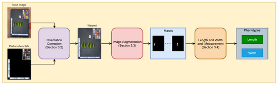
Figure 2.
An overview of the proposed method.
3.2. Orientation Correction
A well-constructed imagery platform where the camera is installed in a way to capture a birds-eye view of the sampling board is costly and sometimes impractical when mobility is required (e.g., capturing images on the field). We relax the constraint of camera pose by proposing the orientation correction module. The purpose of this module is to re-align the input image using the platform template as a reference, hence simplifying the downstream processing modules. Specifically, from the resolution of the platform template image and the rulers on the platform, we can deduct the pixel-to-length constant (cm/pixels) of the platform template to convert any measurements in pixels to centimeters as follows:
where and are measurements in centimeters and pixels, respectively. Since the input image is warped according to the template, we can apply Equation (1) to any measurements from the warped image.
Under the assumption of the pinhole camera model, two images of the same scene are related through a homography matrix H, if either the scene is planar or the camera motion is purely rotational [17]. The homography matrix H is a matrix with 8 degrees of freedom (DoF), which maps a point of a source image to a point in the target image , as follows:
Since the platform we use is a flat surface, we can employ homography transformation (also called perspective transformation) to warp an input image to match the view of the platform template according to Equation (2).
Estimating the homography matrix is a well-established topic in the computer vision field. Traditionally, the homography estimation framework consists of three steps: keypoint detection and correspondence matching, followed by direct linear transformation (DLT). Handcrafted features such as SIFT [18], SURF [19], and ORB [20] are often used to extract and match keypoints. Direct linear transformation is used to solve a linear system of equations constructed from correspondence pairs of two views to obtain a homography matrix H. More recent research on homography estimation is deep-learning-based. Direct regression methods [21,22,23] regress 4-point homography directly from a pair of images and achieve comparable performance with handcrafted features methods. A major drawback of direct regression methods is that 4-point homography representation breaks spatial structures. In [24], the authors propose a perspective field (PFNet) to predict bijective pixel-to-pixel linear mapping to address the drawback of direct regression methods. PFNet [24] achieves robustness to different lighting conditions but not for big viewpoint changes [25]. Applying perceptual loss [25] functions helps decouple presentation for homography estimation and image comparison, hence improving the robustness for both lightning conditions and big changes in viewpoint. SuperGlue [14] proposes learning feature matching using an attention graph neural network, and when combined with SuperPoint [26], it achieves good performance for both indoor and outdoor images.
We select SuperGlue [14] for homography estimation because its pretrained model is available and performs well for both indoor and outdoor scenes. Figure 3 illustrates the flow of the orientation correction module. Initially, an image of cucumber samples and a platform template serve as an image pair. Subsequently, corresponding point pairs between the two input images are generated using the SuperGlue algorithm. These correspondences are then utilized to estimate the homography matrix H between the two views. Finally, the image of cucumbers is warped using the perspective transformation with the homography matrix H.
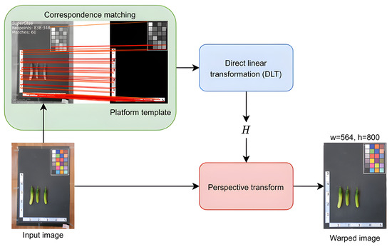
Figure 3.
Orientation correction module.
3.3. Image Segmentation
We create an effective zero-shot framework for segmenting cucumbers from an image by combining two widely used zero-shot models: segment anything (SAM) [15] and contrastive language–image pretraining (CLIP) [16]. Figure 4 illustrates an overview of the proposed image segmentation pipeline, which consists of two steps: (i) obtaining object masks via SAM (Figure 4a) and (ii) classifying segmented objects with CLIP (Figure 4c) and only keeping objects that are classified as a cucumber.
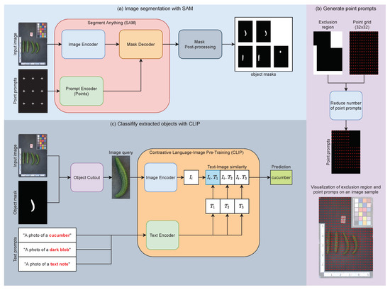
Figure 4.
Image segmentation pipeline with SAM and CLIP.
Image Segmentation with SAM: Segment anything (SAM), developed by [15], stands as a state-of-the-art foundational model for image segmentation and offers several pretrained models trained on the extensive SA-1B dataset, comprising more than 1 billion masks from 11 million images. The SAM model architecture consists of three key modules: an image encoder, a prompt encoder, and a mask decoder (see Figure 4a). The image encoder takes an input image and produces an image embedding. The prompt encoder can handle two types of prompts: sparse (points, boxes, and texts) and dense (masks). By combining the image and prompt embeddings, the mask decoders generate masks for segmentation. Since prior knowledge of the cucumber’s location in the input image is unavailable, a 32 × 32 point grid is employed as an input prompt to extract masks. Additionally, the input image is warped according to the template, allowing for the definition of exclusion regions in the phenotyping platform where the cucumber is not present. Further improvements to the prompts can be achieved by eliminating point prompts in these exclusion regions. This prompt generation pipeline is shown in Figure 4b. However, when using point grids as input prompts, the obtained masks include many duplicate masks and noise blobs from the background. To address this, we filter these masks by removing those that are too small or too large and merging masks that are duplicated or highly overlapping. Specifically, we employ a mask post-processing module to process masks resulting from the SAM model. The outputs of the mask post-processing module consist of masks with sizes that fall within the range of 0.05% to 50% of the image area. For merging duplicated masks, we set both the overlap threshold and the Intersection over Union (IoU) threshold to 0.9. Details about the mask post-processing steps can be found in the pseudo-code provided in Algorithm 1.
| Algorithm 1 Mask post-processing |
|
Classify segmented objects with CLIP: Despite the mask post-processing step on SAM outputs, the obtained masks still contain many unwanted objects, such as black blobs from the backgrounds and sample identifiers. To filter out these unwanted masks, we employ CLIP to classify all segmented objects. Contrastive language–image pretraining (CLIP) [16] is a foundation model for text–image pairs that achieves remarkable performance on zero-shot classification tasks. The CLIP model consists of two modules: an image encoder and a text encoder. A classification pipeline for segmented objects is shown in Figure 4c. We extract object images from the input image using the masks obtained from SAM and the post-processing pipeline and then feed them to CLIP’s image encoder to create image embeddings . To generate the text embeddings, we define several text prompts in the format “A photo of an [object class]” where object classes are [“cucumber”, “dark blob”, “text note”]. These text prompts are input to the text encoders, resulting in text embeddings . Next, we calculate the cosine similarity between the image embedding and the text embeddings. The predicted class for each segmented object is determined as . We only kept the segmented objects with the predicted class “cucumber” and discarded the rest.
3.4. Measuring Length and Width
After obtaining the masks from the previous steps, we can measure the width and height of cucumbers from the obtained masks. The length of a cucumber is defined as the length of the predominant medial axis segment excluding the stem part (see Figure 5). However, defining the width of a cucumber is not straightforward, as there are an infinite number of lines perpendicular to the medial axis. Therefore, we propose profiling the width of cucumber by measuring it at various points along the medial axis , as shown in Figure 6. If a single value to represent the width of a sample is desired, we can use the median of width profile .
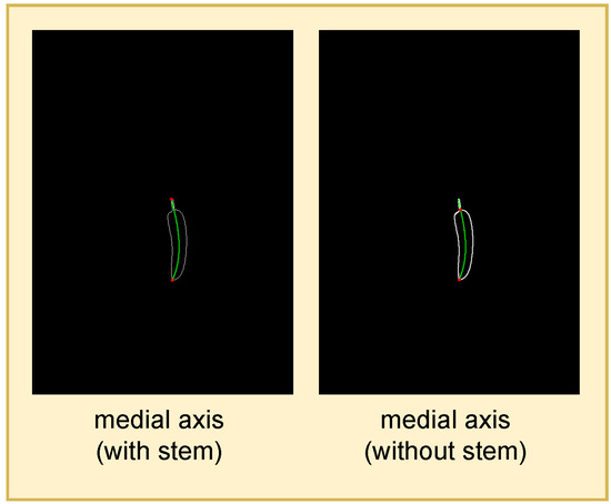
Figure 5.
Cucumber length is defined as the length of the medial axis segment without stem. The medial axis segments are denoted as green curves, and their endpoints are highlighted as red dots.
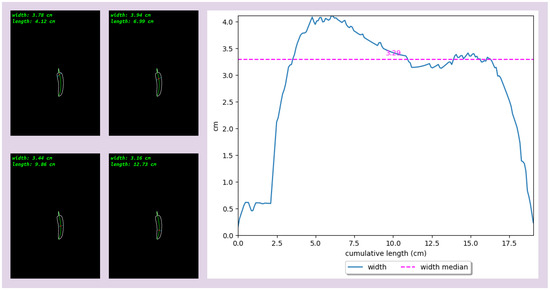
Figure 6.
The width of a sample is measured along its medial axis, and the values of the width are plotted against the cumulative length along the medial axis.
An overview of the measuring pipeline is illustrated in Figure 7. Starting with an input mask obtained from the image segmentation step, a morphological skeletonization [27] is applied to the input masks to reduce the binary masks to a 1-pixel-wide skeleton, also known as the medial axis. Next, we parameterize the skeleton as a B-spline curve [28] and then proceed to profile the input mask along the B-spline medial axis. The width of a cucumber sample is calculated from its mask’s width profile, as mentioned above. From the width profile, we can detect the transition point between the stem part and the body part, which is referred to as the stem point. Finally, the length of a cucumber is determined as the length of the medial axis curve segment between the stem point and one end of the medial axis.
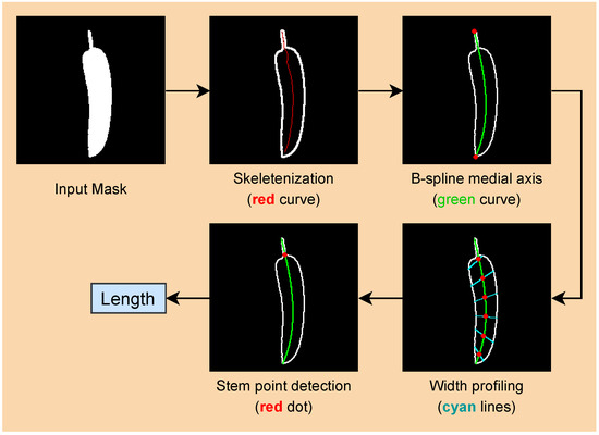
Figure 7.
Width and height measurement pipeline.
A B-spline is a piecewise polynomial function that is commonly used in many fields for curve and surface representation. A B-spline curve of degree k is defined using control points as follows:
where the basis function is often defined recursively using the Cox-de Boor formula:
and
Each scalar is called a knot, and the knot sequence is nondecreasing, which means .
Given a set of m data points , with each represented as a 2D point, we can fit a bivariate B-spline curve to the data P, resulting in a smooth curve that fits the input data. A B-spline curve is parameterized via knott, and a point on a bivariate B-spline curve is defined by . Consequently, the order of points in data can significantly influence the resulting B-spline curve. Unfortunately, the skeleton image only provides the locations of points on the medial axis, not the sequence in which the points appear. Additionally, the skeleton obtained from morphological operations may contain several branches and noise, depending on the shape of the input binary mask. To ensure consistency when constructing the B-spline medial axis, the data P must only contain the points of the main branch. We address these two problems by constructing path graph from the list of data points P.
In graph theory, a path graph is a simple graph that consists of a single chain of nodes connected by edges. In other words, a path graph contains exactly two leaf nodes (node degree = 1), while the other nodes have exactly two neighbor nodes (node degree = 2), and does not have self-loop edges. We use Algorithm 2 to construct the path graph from a skeleton image. Algorithm 2 starts with collecting all foreground pixels from a binary morphological skeleton image. Then, we construct a radius graph from the set of foreground pixels and with a radius r. The radius graph takes in all the points in as nodes and connects to two nodes if the euclidean distance between them is less than r. Assuming the skeleton is continuous, due to the discreteness of the pixel grid, the maximum distance between two adjacent pixels is , and the minimum distance between two non-adjacent pixels is 2. Therefore, by selecting , the radius graph only connects adjacent pixels. The next step is finding the leaf nodes in the radius graph by calculating the nodes’ degrees. The degree of a node is the number of edges connected to it. Hence, a leaf node that has a degree of 1 can be used to determine the start or end point of a path.
Let be the adjacency matrix of the radius graph , where an element of the adjacency matrix A represents the edge value between nodes u and v. indicates that node u is connected to node v, while indicates no connection between the nodes. The degree (excluding self-loop) of a node u can be calculated as follows:
If the number of leaf nodes in the radius graph is 2, has only one branch, making it a path graph. When there are more than two leaf nodes, it indicates that the radius graph contains multiple branches. As mentioned earlier, utilizing the main branch enhances the consistency of medial axis estimation. The main branch is defined as the longest path that starts from one leaf node and ends at another leaf node. By calculating the path lengths for every possible pair of leaf nodes, we can determine the main branch as the longest one. The length of a branch is defined as the shortest route to travel from one of its leaf nodes to another leaf node.
| Algorithm 2 Constructing path graph from skeleton |
|
Once the path graph is created, a B-spline curve is obtained by fitting it to . The B-spline curve is parameterized by , where and are associated with the two ends of the B-spline curves, which are closely fit to the two leaf nodes of . As discussed above, the skeleton obtained from the morphology process does not touch the boundary of the binary mask. Therefore, the length of the B-spline curve segment with is always less than the actual length of the cucumber. Therefore, we extend the range of knot values from to with a small constant . In essence, this means we extend the polynomial curves at the two ends of the B-spline curve with . We can find the two end points of the cucumber as the intersections of the extended B-spline curve and the boundary of the input mask. Then, we add the two new end points to the path graph and construct a new B-spline curve . The new B-spline curve is parameterized via , with and corresponding to the two ends of the cucumber mask. The length of the cucumber including the stem part is calculated as:
where , and the interval . Equation (7) can be approximated using the chord length method. Similarly, we can calculate the length of a cucumber excluding the stem part by finding the transition point between the stem and body of a cucumber and using Equation (7) with the interval .
We detect the stem parts of a cucumber based on two observations. Firstly, many cucumber samples come with long and narrow stems. For this kind of sample, the transition from the stem part to the body part is abrupt, which reflects on the width profile as a spike in the change in width (see Figure 8a). We can detect the transition point by detecting the peak of the width change rate. The width change rate is calculated as follows:
where is the width of a cucumber measured at the i-th position of the medial axis, and . Consequently, the peak of the width change rate is calculated as . If , where is a hyperparameter and is the width median, a cucumber has a long and narrow stem, and the transition point is at the peak width change rate (see Figure 8a). Otherwise, the cucumber either comes with a short and thick stem or does not have one (see Figure 8b). In this case, the stem is determined via its relative width compared to the cucumber width. Specifically, we use a hyperparameter to calculate the maximum stem width and use it as a threshold to determine the transition point (see Figure 8b). To find the optimal values for and , we perform a grid search on the test set, and the results are shown in Table 1. As can be seen from Table 1, the optimal parameters are and .
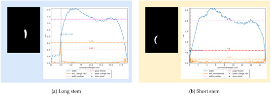
Figure 8.
Detecting stem via width profile.

Table 1.
Finding the optimal values for and using grid search. We report the MAPE of the predictions against the ground truth. The best MAPE value is highlighted in bold.
4. Results
4.1. Dataset
To test the effectiveness of the proposed method, we created a small test set comprising 90 images, each containing 412 cucumber samples. We manually measured the length of each sample using the popular open-source software ImageJ [29]. We manually labeled the medial axis for each of the cucumber samples by drawing a polyline and used the rulers in the image to estimate the pixel-to-length constant . The length of the medial axis is then calculated automatically via ImageJ software.
4.2. Results on Length Measurement
In Section 3.4, we discuss the limitations of morphological skeletons, which are clearly visualized in Figure 9. The morphological skeletons often do not intersect with the masks’ boundaries. Furthermore, they are sensitive to noise, resulting in skeletons with several branches and a lack of smoothness. In contrast, our utilization of B-spline medial axes yields a successful, closely fitted solution that effectively addresses the shortcomings of the morphological skeletons. Figure 9 also demonstrates the effectiveness of our proposed method in detecting the stem part of the cucumbers.
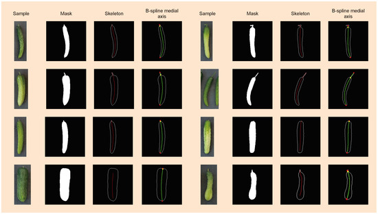
Figure 9.
Visualization of the measurement pipeline that takes in an input mask, estimates the B-spline medial axis, and then detects the stem part. The two end points of the B-spline medial axis are highlighted as red dots, and the transition point between the stem part and body part is highlighted as yellow dots.
In essence, the proposed method is equivalent to manual measurement when determining the length of a cucumber, with the distinction that all steps are automated. When measuring manually, the medial axis is approximated using about 6 to 10 line segments, whereas in our approach, we divide the B-spline medial axis into 200 line segments before calculating its length using the chord length method. This approach reduces the quantization error caused by a small number of line segments.
Figure 10 displays the error distribution of length measurements when combining all modules. As shown in Figure 10, the proposed method achieves a MAPE of 2.20%, and 92.96% of the samples have an error within . The method performs particularly well on larger samples. Upon investigating the cases of failure, we discovered that most errors stem from the detection of the stem part. Detecting the stem part in unripe cucumber samples poses a particular challenge because the width of the stem part is very similar to that of the body part. Addressing this problem fully would require a supervised machine learning method, which we leave for future work.
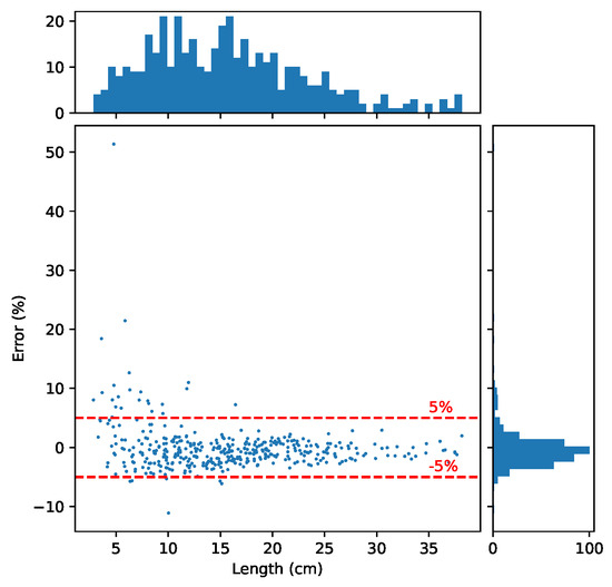
Figure 10.
Error distribution on the test set. The histogram on top size shows the size in length distribution the samples. The histogram on the right size illustrates the distribution of the error (%). The main plot shows the relationship between the error (%) and the size of the samples.
5. Conclusions
In this study, we have introduced a straightforward yet highly effective framework for the measurement of essential cucumber phenotypes, specifically focusing on length and width. Our framework leverages recent advancements in deep learning models, particularly in image registration, segmentation, and classification, which have granted pretrained models the remarkable ability for zero-shot learning. By harnessing the power of these models, we have devised a cucumber phenotyping system that stands out for its ability to operate without the need for labeled data or model training.
One of the noteworthy innovations we propose in this framework is the utilization of a B-spline curve as the medial axis. This decision has proven to be instrumental in enhancing our ability to accurately measure the length and width of cucumbers. The B-spline curve not only provides a robust representation of cucumber morphology but also aids in overcoming the challenges associated with accurately measuring these traits. Our results demonstrate that our approach achieves significant success in predicting cucumber phenotypes, as exemplified by a MAPE of 2.20%. Furthermore, 92.96% of the samples have an error rate of less than 5%, highlighting the reliability of our method, particularly on larger samples. However, it is crucial to acknowledge that challenges remain, especially concerning the accurate detection of the stem part in unripe cucumber samples. The similarity in width between the stem and body parts poses a unique challenge that warrants further attention. To fully address this issue, a supervised machine learning method may be necessary. While we leave the development of such an algorithm to future work, it represents an essential avenue for continued research in cucumber phenotyping.
Each type of plant has a different shape, thus requiring different specifications for measurement. Since our measuring pipeline is tailored for cucumbers, it cannot be applied directly to other plants. Nevertheless, there are a few takeaways from the research that can be used to develop measurement pipelines for different plants. Firstly, we propose a template-based orientation correction module to warp the input image to match the orientation of the template. This is a cost-effective alternative compared to building a sophisticated phenotyping platform and can be trivially applied to different template designs. Secondly, we propose a zero-shot segmentation module using SAM and CLIP. This approach is suitable when the color and texture of the object of interest are fairly consistent and distinguishable from the background. This assumption is reasonable since we can always design an appropriate template tailored specifically to the object of interest, and the orientation module does not require any specific template. Finally, we propose using a B-spline curve to improve the consistency of length measurement, which is robust to noise from segmentation results. Therefore, it is a better alternative compared to directly using the morphological skeleton. This insight can be applied to other plant phenotyping methods that are based on the morphological skeleton to extract the medial axis.
In conclusion, our proposed trait measurement framework represents a significant step forward in cucumber phenotyping. By capitalizing on recent advances in deep learning and innovative techniques like the B-spline curve, we have achieved highly accurate results without the need for extensive labeled data or model training. Nevertheless, we recognize the ongoing challenges, particularly in stem part detection, and look forward to future advancements in this field.
Author Contributions
Conceptualization, H.Y.P. and O.N.L.; methodology, L.Q.N.; validation, L.M.D. and O.N.L.; data curation, H.Y.P. and L.Q.N.; writing—original draft preparation, L.Q.N., S.R. and J.S.; writing—review and editing, H.M.; visualization, J.S.; supervision, H.M.; funding acquisition, H.Y.P. and H.M. All authors have read and agreed to the published version of the manuscript.
Funding
This work was supported by the National Research Foundation of Korea (NRF) grant funded by the Korean government, the Ministry of Science and ICT (MSIT) (2021R1F1A1046339), and by the Korea Institute of Planning and Evaluation for Technology in Food, Agriculture, Forestry and Fisheries (IPET) through the Digital Breeding Transformation Technology Development Program, funded by the Ministry of Agriculture, Food and Rural Affairs (MAFRA) (322063-03-1-SB010), and by the Institute of Information & Communications Technology Planning & Evaluation (IITP) under the Metaverse support program to nurture the best talents (IITP-2023-RS-2023-00254529) grant funded by the Korean Government (MSIT).
Data Availability Statement
Data are available upon request due to restrictions of privacy.
Conflicts of Interest
The authors declare no conflict of interest.
References
- Aglawe, S.B.; Singh, M.; Rama Devi, S.; Deshmukh, D.B.; Verma, A.K. Genomics Assisted Breeding for Sustainable Agriculture: Meeting the Challenge of Global Food Security. In Bioinformatics for Agriculture: High-Throughput Approaches; Springer: Singapore, 2021; pp. 23–51. [Google Scholar]
- Wu, S.; Wen, W.; Xiao, B.; Guo, X.; Du, J.; Wang, C.; Wang, Y. An accurate skeleton extraction approach from 3D point clouds of maize plants. Front. Plant Sci. 2019, 10, 248. [Google Scholar] [CrossRef]
- Wang, Y.; Wen, W.; Wu, S.; Wang, C.; Yu, Z.; Guo, X.; Zhao, C. Maize plant phenotyping: Comparing 3D laser scanning, multi-view stereo reconstruction, and 3D digitizing estimates. Remote. Sens. 2018, 11, 63. [Google Scholar] [CrossRef]
- Wu, S.; Wen, W.; Gou, W.; Lu, X.; Zhang, W.; Zheng, C.; Xiang, Z.; Chen, L.; Guo, X. A miniaturized phenotyping platform for individual plants using multi-view stereo 3D reconstruction. Front. Plant Sci. 2022, 13, 897746. [Google Scholar] [CrossRef]
- Dang, L.M.; Min, K.; Nguyen, T.N.; Park, H.Y.; Lee, O.N.; Song, H.K.; Moon, H. Vision-Based White Radish Phenotypic Trait Measurement with Smartphone Imagery. Agronomy 2023, 13, 1630. [Google Scholar] [CrossRef]
- Dang, L.M.; Nadeem, M.; Nguyen, T.N.; Park, H.Y.; Lee, O.N.; Song, H.K.; Moon, H. VPBR: An Automatic and Low-Cost Vision-Based Biophysical Properties Recognition Pipeline for Pumpkin. Plants 2023, 12, 2647. [Google Scholar] [CrossRef] [PubMed]
- Liu, L.; Yu, L.; Wu, D.; Ye, J.; Feng, H.; Liu, Q.; Yang, W. PocketMaize: An android-smartphone application for maize plant phenotyping. Front. Plant Sci. 2021, 12, 770217. [Google Scholar] [CrossRef] [PubMed]
- He, K.; Gkioxari, G.; Dollár, P.; Girshick, R. Mask r-cnn. In Proceedings of the CVPR, Honolulu, HI, USA, 21–26 July 2017; pp. 2961–2969. [Google Scholar]
- Wang, X.; Zhang, R.; Kong, T.; Li, L.; Shen, C. Solov2: Dynamic and fast instance segmentation. Adv. Neural Inf. Process. Syst. 2020, 33, 17721–17732. [Google Scholar]
- Chen, L.C.; Zhu, Y.; Papandreou, G.; Schroff, F.; Adam, H. Encoder-decoder with atrous separable convolution for semantic image segmentation. In Proceedings of the ECCV, Munich, Germany, 8–14 September 2018; pp. 801–818. [Google Scholar]
- Nguyen, T.N.; Nguyen-Xuan, H.; Lee, J. A novel data-driven nonlinear solver for solid mechanics using time series forecasting. Finite Elem. Anal. Des. 2020, 171, 103377. [Google Scholar] [CrossRef]
- Nguyen, T.N.; Lee, S.; Nguyen, P.C.; Nguyen-Xuan, H.; Lee, J. Geometrically nonlinear postbuckling behavior of imperfect FG-CNTRC shells under axial compression using isogeometric analysis. Eur. J. Mech.-A/Solids 2020, 84, 104066. [Google Scholar] [CrossRef]
- Zenkl, R.; Timofte, R.; Kirchgessner, N.; Roth, L.; Hund, A.; Van Gool, L.; Walter, A.; Aasen, H. Outdoor plant segmentation with deep learning for high-throughput field phenotyping on a diverse wheat dataset. Front. Plant Sci. 2022, 12, 774068. [Google Scholar] [CrossRef] [PubMed]
- Sarlin, P.E.; DeTone, D.; Malisiewicz, T.; Rabinovich, A. Superglue: Learning feature matching with graph neural networks. In Proceedings of the CVPR, Virtual, 14–19 June 2020; pp. 4938–4947. [Google Scholar]
- Kirillov, A.; Mintun, E.; Ravi, N.; Mao, H.; Rolland, C.; Gustafson, L.; Xiao, T.; Whitehead, S.; Berg, A.C.; Lo, W.Y.; et al. Segment anything. arXiv 2023, arXiv:2304.02643. [Google Scholar]
- Radford, A.; Kim, J.W.; Hallacy, C.; Ramesh, A.; Goh, G.; Agarwal, S.; Sastry, G.; Askell, A.; Mishkin, P.; Clark, J.; et al. Learning transferable visual models from natural language supervision. In Proceedings of the ICML, PMLR, Virtual, 18–24 July 2021; pp. 8748–8763. [Google Scholar]
- Hartley, R.; Zisserman, A. Multiple View Geometry in Computer Vision; Cambridge University Press: Cambridge, UK, 2003. [Google Scholar]
- Lowe, D.G. Distinctive image features from scale-invariant keypoints. Int. J. Comput. Vis. 2004, 60, 91–110. [Google Scholar] [CrossRef]
- Bay, H.; Tuytelaars, T.; Van Gool, L. Surf: Speeded up robust features. Lect. Notes Comput. Sci. 2006, 3951, 404–417. [Google Scholar]
- Rublee, E.; Rabaud, V.; Konolige, K.; Bradski, G. ORB: An Efficient Alternative to SIFT or SURF. In Proceedings of the ICCV, Barcelona, Spain, 6–13 November 2011; pp. 2564–2571. [Google Scholar]
- DeTone, D.; Malisiewicz, T.; Rabinovich, A. Deep image homography estimation. arXiv 2016, arXiv:1606.03798. [Google Scholar]
- Erlik Nowruzi, F.; Laganiere, R.; Japkowicz, N. Homography estimation from image pairs with hierarchical convolutional networks. In Proceedings of the ICCV Workshops, Venice, Italy, 22–29 October 2017; pp. 913–920. [Google Scholar]
- Nguyen, T.; Chen, S.W.; Shivakumar, S.S.; Taylor, C.J.; Kumar, V. Unsupervised deep homography: A fast and robust homography estimation model. IEEE Robot. Autom. Lett. 2018, 3, 2346–2353. [Google Scholar] [CrossRef]
- Zeng, R.; Denman, S.; Sridharan, S.; Fookes, C. Rethinking planar homography estimation using perspective fields. In Proceedings of the ACCV, Perth, Australia, 2–6 December 2018; Springer: Cham, Switzerland, 2018; pp. 571–586. [Google Scholar]
- Koguciuk, D.; Arani, E.; Zonooz, B. Perceptual loss for robust unsupervised homography estimation. In Proceedings of the CVPR, Virtual, 19–25 June 2021; pp. 4274–4283. [Google Scholar]
- DeTone, D.; Malisiewicz, T.; Rabinovich, A. Superpoint: Self-supervised interest point detection and description. In Proceedings of the CVPR Workshops, Salt Lake City, UT, USA, 18–22 June 2018; pp. 224–236. [Google Scholar]
- Zhang, T.Y.; Suen, C.Y. A fast parallel algorithm for thinning digital patterns. Commun. ACM 1984, 27, 236–239. [Google Scholar] [CrossRef]
- Dierckx, P. Curve and Surface Fitting with Splines; Oxford University Press: Oxford, UK, 1995. [Google Scholar]
- Schneider, C.A.; Rasband, W.S.; Eliceiri, K.W. NIH Image to ImageJ: 25 years of image analysis. Nat. Methods 2012, 9, 671–675. [Google Scholar] [CrossRef] [PubMed]
Disclaimer/Publisher’s Note: The statements, opinions and data contained in all publications are solely those of the individual author(s) and contributor(s) and not of MDPI and/or the editor(s). MDPI and/or the editor(s) disclaim responsibility for any injury to people or property resulting from any ideas, methods, instructions or products referred to in the content. |
© 2023 by the authors. Licensee MDPI, Basel, Switzerland. This article is an open access article distributed under the terms and conditions of the Creative Commons Attribution (CC BY) license (https://creativecommons.org/licenses/by/4.0/).