
A Light-Weighted Machine Learning Approach to Channel Estimation for New-Radio Systems


Abstract
:1. Introduction
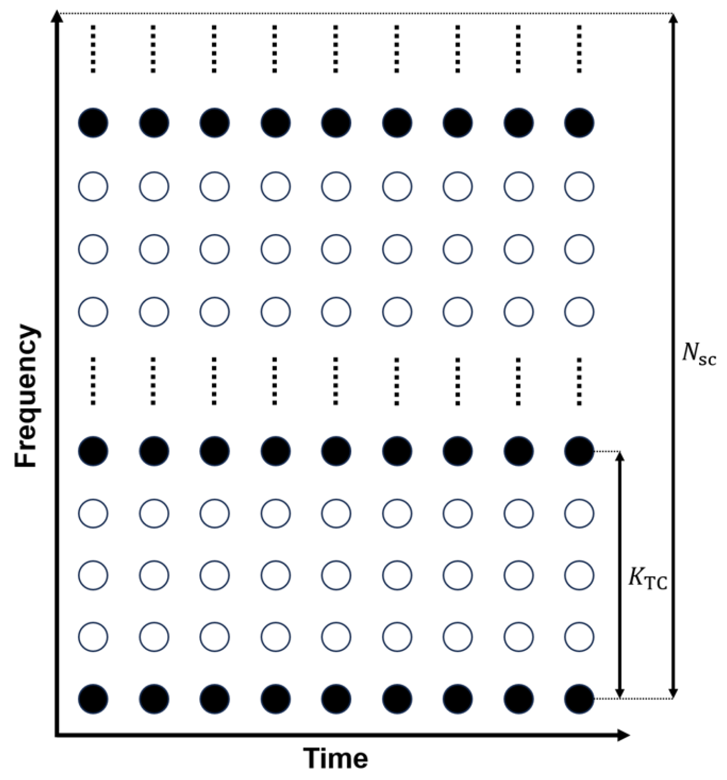
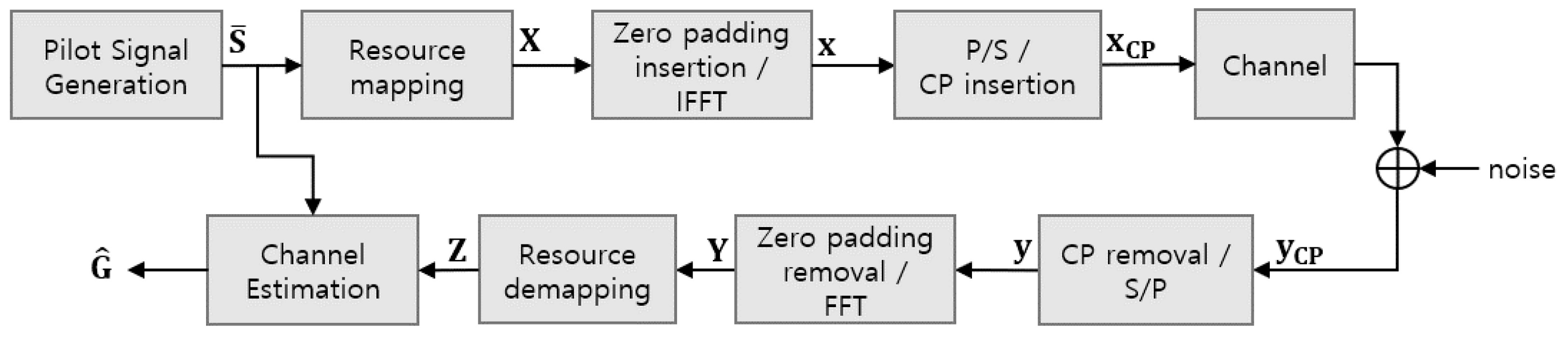
2. System Model
3. Preliminaries on Channel Estimation
3.1. LS/MMSE Method
3.2. Existing ML Method
3.2.1. Structure
3.2.2. Activation Function
4. Proposed ML Method
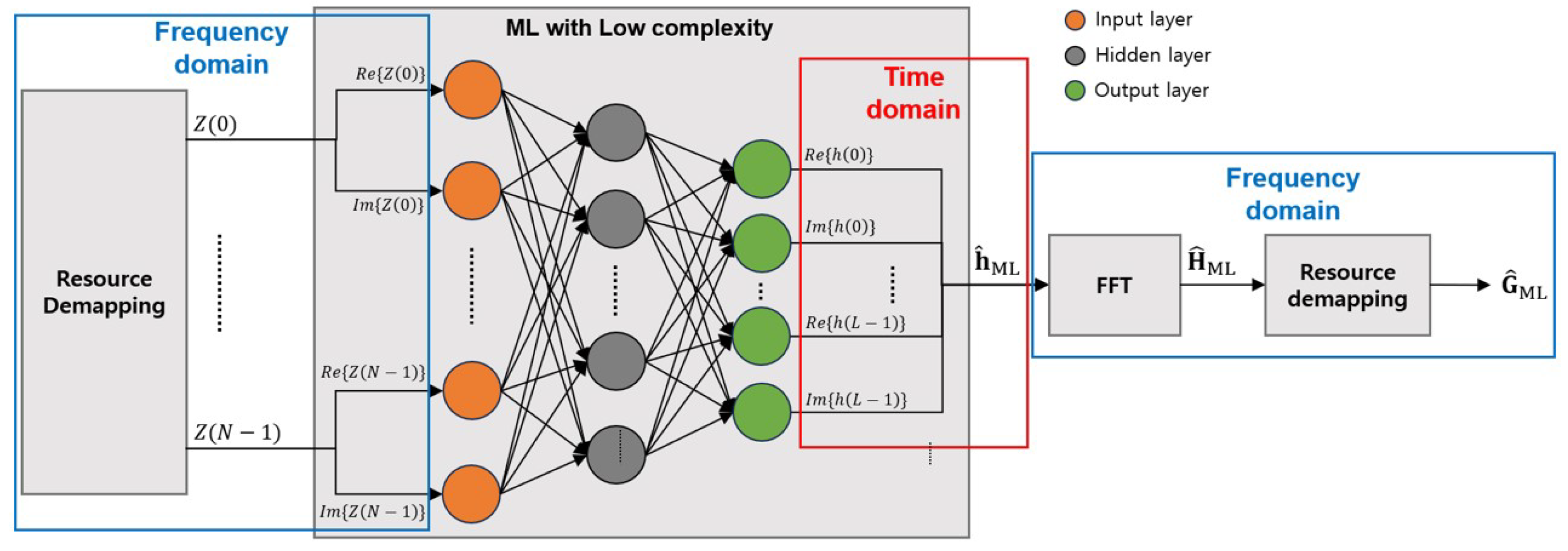
4.1. Network Architecture
4.1.1. Structure
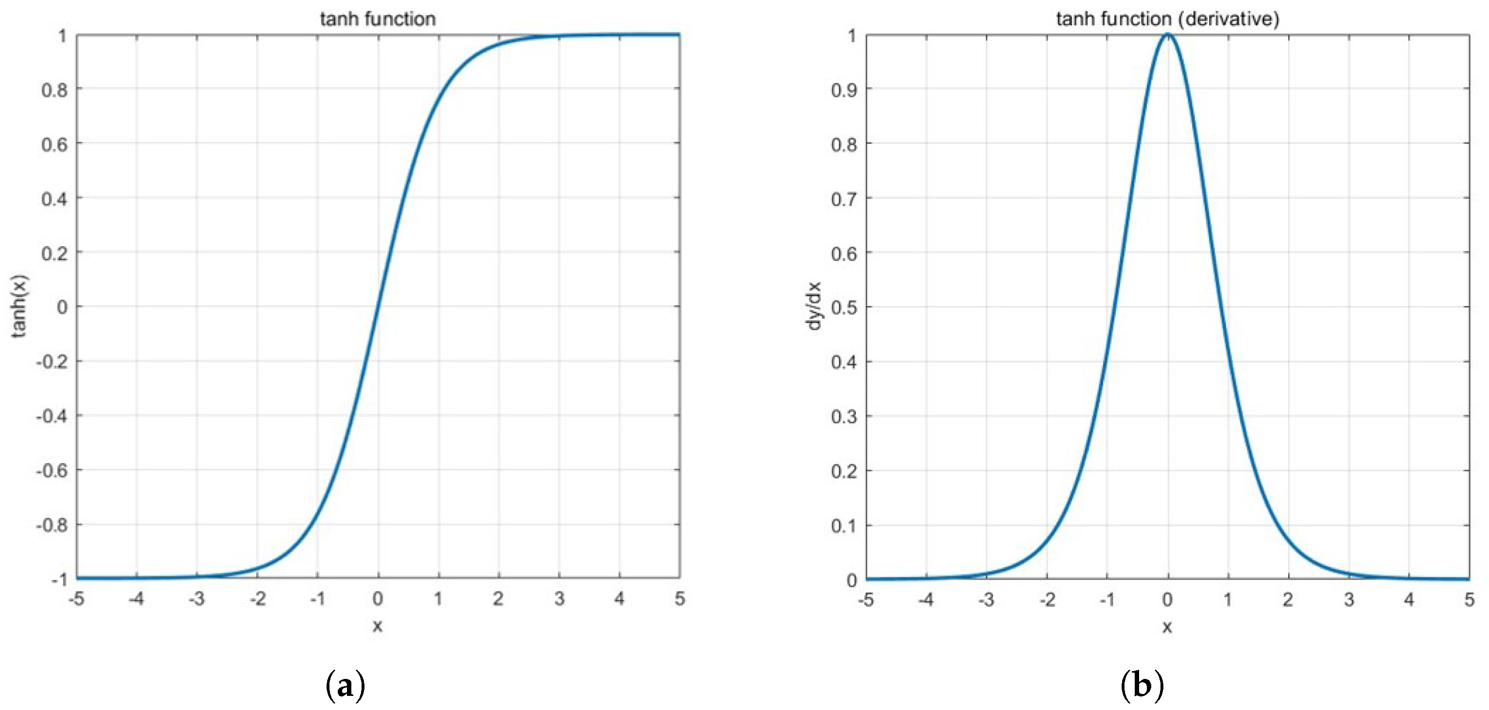
4.1.2. Activation Function
4.1.3. Complexity Analysis
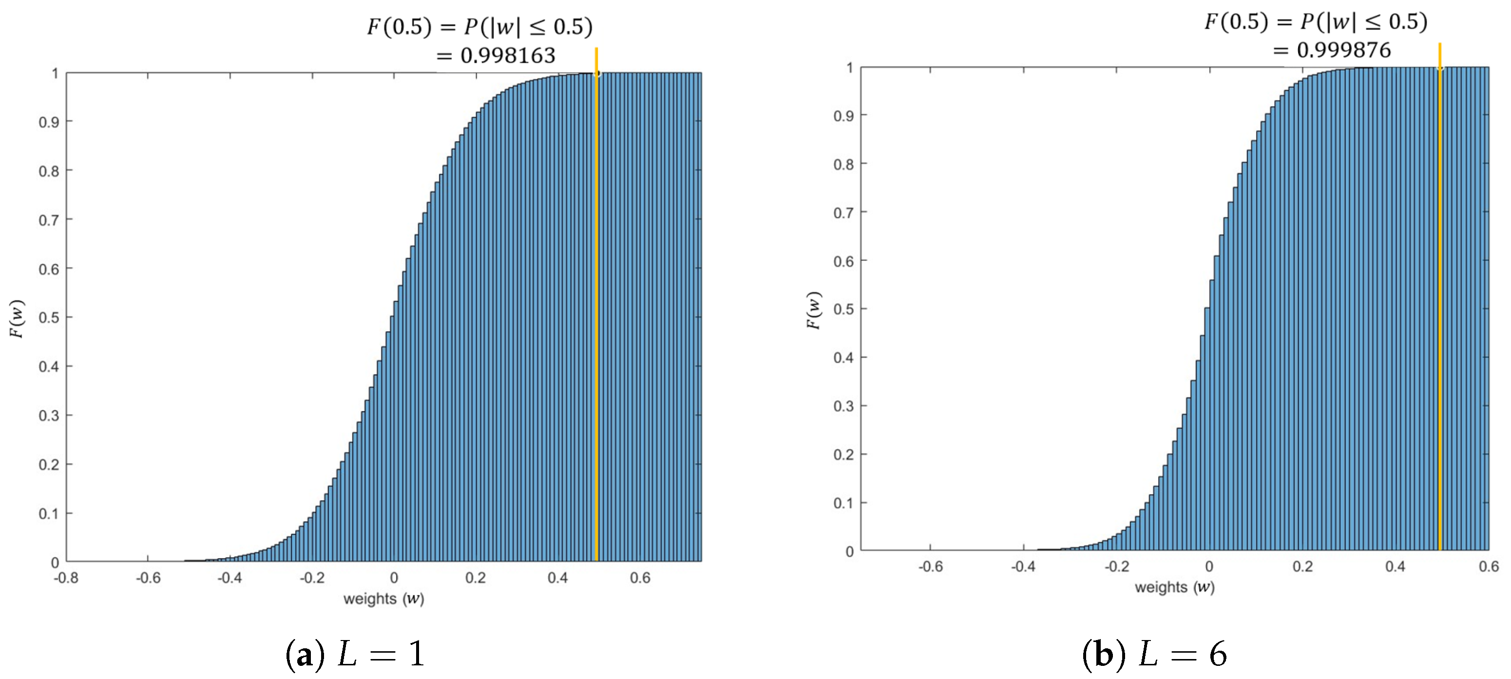
4.2. Quantization Method
5. Simulation Analysis
5.1. Simulation Environment
5.2. Simulation Results
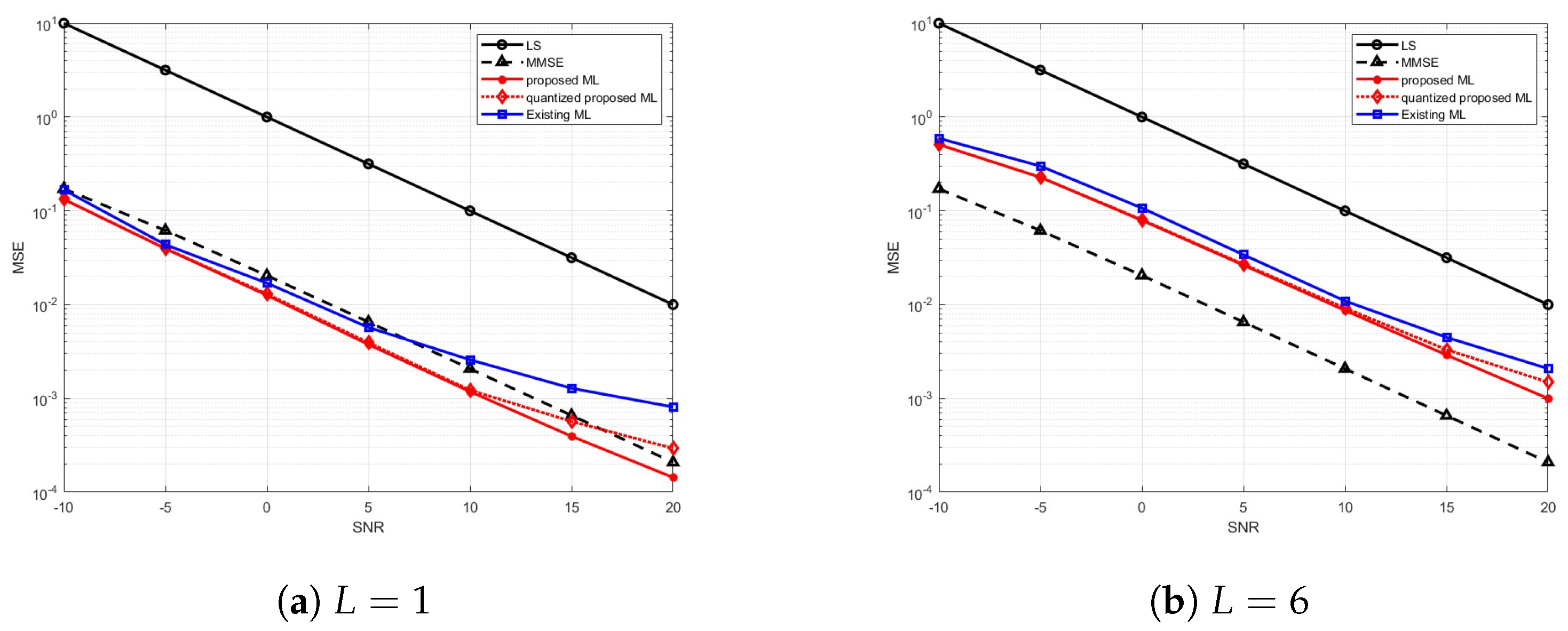
5.2.1. Comparison between Existing Methods and Proposed Method
5.2.2. The Number of Hidden Layers
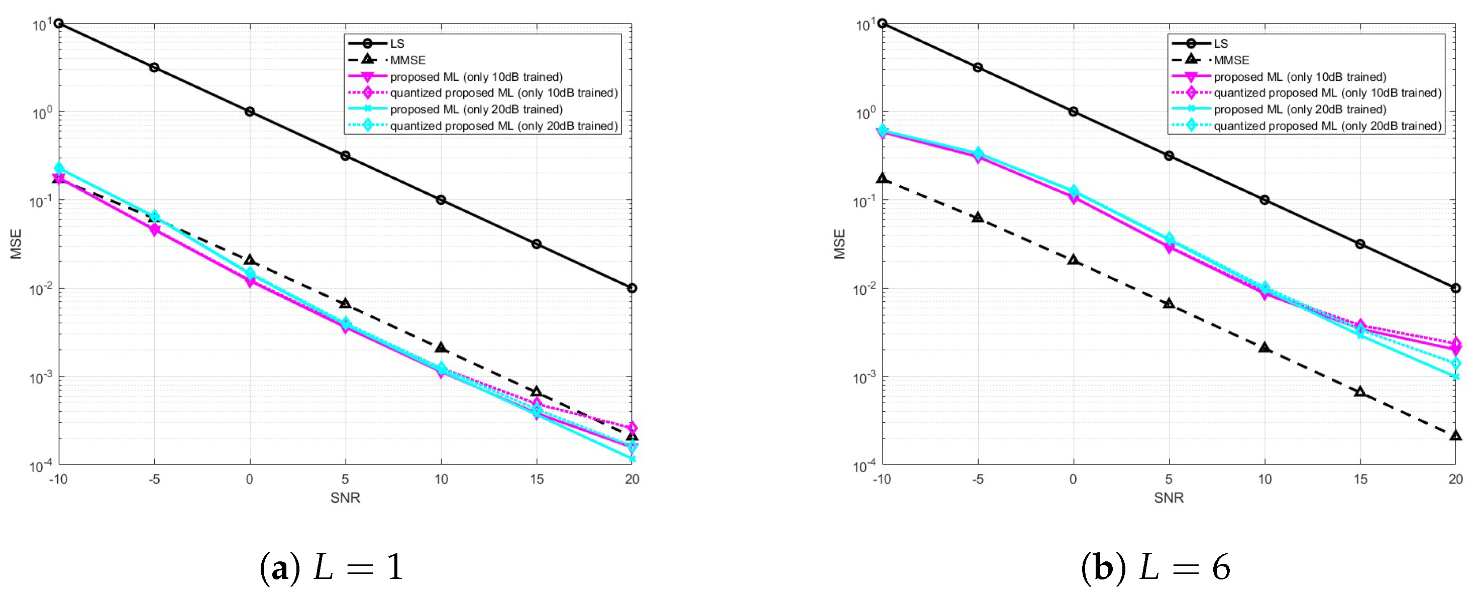
5.2.3. ML Robustness to Other SNRs
6. Conclusions
Author Contributions
Funding
Institutional Review Board Statement
Informed Consent Statement
Data Availability Statement
Conflicts of Interest
Abbreviations
| 3GPP | 3rd Generation Partnership Project |
| 5G | 5th Generation |
| AWGN | Additive White Gaussian Noise |
| CFR | Channel Frequency Response |
| CIR | Channel Impulse Response |
| CNN | Convolutional Neural Network |
| CP | Cylic-Prefix |
| DMRS | DeModulation Reference Signal |
| DNN | Deep NN |
| FFT | Fast Fourier Transform |
| IFFT | Inverse FFT |
| i.i.d. | Independent and Identically Distributed |
| LSTM | Long Short-Term Memory |
| ML | Machine Learning |
| MNN | Multi-Layer NN |
| MSE | Mean Square Error |
| NR | New-Radio |
| OFDMA | Orthogonal Frequency Division Multiple Access |
| PAPR | Peak-to-Average Power Ratio |
| SRS | Sounding Reference Signal |
| ZP | Zero Padding |
References
- Hou, X.; Zhang, Z.; Kayama, H. DMRS Design and Channel Estimation for LTE-Advanced MIMO Uplink. In Proceedings of the 2009 IEEE 70th Vehicular Technology Conference Fall, Anchorage, AK, USA, 20–23 September 2009; pp. 1–5. [Google Scholar]
- Wang, Y.; Zheng, A.; Zhang, J.; Yang, D. A novel channel estimation algorithm for sounding reference signal in LTE uplink transmission. In Proceedings of the 2009 IEEE International Conference on Communications Technology and Applications, Beijing, China, 16–18 October 2009; pp. 412–415. [Google Scholar]
- Bertrand, P. Channel Gain Estimation from Sounding Reference Signal in LTE. In Proceedings of the 2011 IEEE 73rd Vehicular Technology Conference (VTC Spring), Budapest, Hungary, 15–18 May 2011; pp. 1–5. [Google Scholar]
- Xia, X.; Zhao, H.; Zhang, C. Improved SRS design and channel estimation for LTE-advanced uplink. In Proceedings of the 2013 5th IEEE International Symposium on Microwave, Antenna, Propagation and EMC Technologies for Wireless Communications, Chengdu, China, 29–31 October 2013; pp. 84–90. [Google Scholar]
- Tran, H.; Mai, T.-A.; Dang, S.; Ngo, H.-A. Large-scale MU-MIMO uplink channel estimation using sounding reference signal. In Proceedings of the 2018 2nd International Conference on Recent Advances in Signal Processing, Telecommunications & Computing (SigTelCom), Ho Chi Minh City, Vietnam, 29–31 January 2018; pp. 107–110. [Google Scholar]
- Balevi, E.; Doshi, A.; Andrews, J.G. Massive MIMO Channel Estimation With an Untrained Deep Neural Network. IEEE Trans. Wireless Commun. 2020, 19, 2079–2090. [Google Scholar] [CrossRef]
- Le Ha, A.; Van Chien, T.; Nguyen, T.H.; Choi, W. Deep Learning-Aided 5G Channel Estimation. In Proceedings of the 2021 15th International Conference on Ubiquitous Information Management and Communication (IMCOM), Seoul, Republic of Korea, 4–6 January 2021; pp. 1–7. [Google Scholar]
- Mei, K.; Liu, J.; Zhang, X.; Cao, K.; Rajatheva, N.; Wei, J. A Low Complexity Learning-Based Channel Estimation for OFDM Systems With Online Training. IEEE Trans. Commun. 2021, 69, 6722–6733. [Google Scholar] [CrossRef]
- Ma, X.; Gao, Z. Data-Driven Deep Learning to Design Pilot and Channel Estimator for Massive MIMO. IEEE Trans. Veh. Technol. 2020, 69, 5677–5682. [Google Scholar] [CrossRef]
- Jiang, P.; Wen, C.-K.; Jin, S.; Li, G.Y. Dual CNN-Based Channel Estimation for MIMO-OFDM Systems. IEEE Trans. Commun. 2021, 69, 5859–5872. [Google Scholar] [CrossRef]
- Le, H.A.; Van Chien, T.; Nguyen, T.H.; Choo, H.; Nguyen, V.D. Machine learning-based 5G-and-beyond channel estimation for MIMO-OFDM communication systems. Sensors 2021, 21, 4861. [Google Scholar] [CrossRef] [PubMed]
- Dayi, A.B. Improving 5G NR Uplink Channel Estimation with Artificial Neural Networks: A Practical Study on NR PUSCH Receiver. In Proceedings of the 2022 IEEE International Black Sea Conference on Communications and Networking (BlackSeaCom), Sofia, Bulgaria, 6–9 June 2022; pp. 129–134. [Google Scholar]
- Liao, Y.; Hua, Y.; Cai, Y. Deep Learning Based Channel Estimation Algorithm for Fast Time-Varying MIMO-OFDM Systems. IEEE Commun. Lett. 2020, 24, 572–576. [Google Scholar] [CrossRef]
- Bai, Q.; Wang, J.; Zhang, Y.; Song, J. Deep Learning-Based Channel Estimation Algorithm Over Time Selective Fading Channels. IEEE Trans. Cognit. Commun. Netw. 2019, 6, 125–134. [Google Scholar] [CrossRef]
- Yang, Y.; Gao, F.; Ma, X.; Zhang, S. Deep Learning-Based Channel Estimation for Doubly Selective Fading Channels. IEEE Access 2019, 7, 36579–36589. [Google Scholar] [CrossRef]
- Jebur, B.A.; Alkassar, S.H.; Abdullah, M.A.M.; Tsimenidis, C.C. Efficient Machine Learning-Enhanced Channel Estimation for OFDM Systems. IEEE Access 2021, 9, 100839–100850. [Google Scholar] [CrossRef]
- Han, S.; Mao, H.; Dally, W.J. Deep compression: Compressing deep neural networks with pruning, trained quantization and Huffman coding. arXiv 2015, arXiv:1510.00149. [Google Scholar]
- Gholami, A.; Kim, S.; Dong, Z.; Yao, Z.; Mahoney, M.W.; Keutzer, K. A Survey of Quantization Methods for Efficient Neural Network Inference. arXiv 2021, arXiv:2103.13630. [Google Scholar]
- van de Beek, J.-J.; Edfors, O.; Sandell, M.; Wilson, S.K.; Borjesson, P.O. On channel estimation in OFDM systems. In Proceedings of the 1995 IEEE 45th Vehicular Technology Conference. Countdown to the Wireless Twenty-First Century, Chicago, IL, USA, 25–28 July 1995; pp. 815–819. [Google Scholar]
- Hsieh, M.-H.; Wei, C.-H. Channel estimation for OFDM systems based on comb-type pilot arrangement in frequency selective fading channels. IEEE Trans. Consum. Electron. 1998, 44, 217–225. [Google Scholar] [CrossRef]
- Morelli, M.; Mengali, U. A comparison of pilot-aided channel estimation methods for OFDM systems. IEEE Trans. Signal Process. 2001, 49, 3065–3073. [Google Scholar] [CrossRef]
- Coleri, S.; Ergen, M.; Puri, A.; Bahai, A. Channel estimation techniques based on pilot arrangement in OFDM systems. IEEE Trans. Broadcast. 2002, 48, 223–229. [Google Scholar] [CrossRef]
- Hajizadeh, R.; Mohamedpor, K.; Tarihi, M.R. Channel Estimation in OFDM System Based on the Linear Interpolation, FFT and Decision Feedback. In Proceedings of the 18th Telecommunication forum TELFOR 2010, Serbia, Belgrade, 23–25 November 2010. [Google Scholar]
- 3GPP TS 38.211 v17.3.0; NR Physical Channels and Modulation. European Telecommunications Standards Institute: Sophia Antipolis, France, 2022.
- Kumar, T.A.; Anjaneyulu, L. Channel Estimation Techniques for Multicarrier OFDM 5G Wireless Communication Systems. In Proceedings of the 2020 IEEE 10th International Conference on System Engineering and Technology (ICSET), Shah Alam, Malaysia, 9 November 2020; pp. 98–101. [Google Scholar]
- Cho, Y.S.; Kim, J.; Yang, W.Y.; Kang, C.G. MIMO-OFDM Wireless Communications with MATLAB; John Wiley & Sons: Hoboken, NJ, USA, 2010. [Google Scholar]
- Kingma, D.P.; Ba, J. Adam: A method for stochastic optimization. arXiv 2014, arXiv:1412.6980. [Google Scholar]


| Perspective | Contents |
|---|---|
| Input data type in ML | |
| Design the number of usage symbols according to channel types |
|
| Channel estimation by domain types |
|
| Complexity and MSE performance |
|
| Our work |
|
| Algorithm | The Number of Multiplications/Inversions | Computational Complexity |
|---|---|---|
| LS | ||
| MMSE | ||
| Existing ML | ||
| Proposed ML |
| Parameters | Values |
|---|---|
| SRS size | 48 |
| Subcarrier size | 216 |
| FFT size | 256 |
| Tap size | |
| Channel model | Gaussian channel |
| Noise model | Gaussian noise |
| SNR |
| Parameters | Values |
|---|---|
| Number of hidden layer | 1 |
| Input layer size | 96 |
| Hidden layer size | 32 |
| Output layer size | |
| Batch size | 8 |
| Learning rate | |
| Training epochs | 100 |
| Activation function | tanh |
| Optimizer | Adam |
| Loss function | Mean squared error |
| Layers | 1Tap DNN | 6Tap DNN | ||
|---|---|---|---|---|
| Nodes | Nodes | |||
| Input layer | 96 | - | 96 | - |
| Hidden layer | 32 | tanh | 32 | tanh |
| Ouput layer | 2 | - | 12 | - |
Disclaimer/Publisher’s Note: The statements, opinions and data contained in all publications are solely those of the individual author(s) and contributor(s) and not of MDPI and/or the editor(s). MDPI and/or the editor(s) disclaim responsibility for any injury to people or property resulting from any ideas, methods, instructions or products referred to in the content. |
© 2023 by the authors. Licensee MDPI, Basel, Switzerland. This article is an open access article distributed under the terms and conditions of the Creative Commons Attribution (CC BY) license (https://creativecommons.org/licenses/by/4.0/).
Share and Cite
Lee, H.W.; Choi, S.W. A Light-Weighted Machine Learning Approach to Channel Estimation for New-Radio Systems. Electronics 2023, 12, 4740. https://doi.org/10.3390/electronics12234740
Lee HW, Choi SW. A Light-Weighted Machine Learning Approach to Channel Estimation for New-Radio Systems. Electronics. 2023; 12(23):4740. https://doi.org/10.3390/electronics12234740
Chicago/Turabian StyleLee, Hyun Woo, and Sang Won Choi. 2023. "A Light-Weighted Machine Learning Approach to Channel Estimation for New-Radio Systems" Electronics 12, no. 23: 4740. https://doi.org/10.3390/electronics12234740
APA StyleLee, H. W., & Choi, S. W. (2023). A Light-Weighted Machine Learning Approach to Channel Estimation for New-Radio Systems. Electronics, 12(23), 4740. https://doi.org/10.3390/electronics12234740