A Decoding Method Using Riemannian Local Linear Feature Construction for a Lower-Limb Motor Imagery Brain–Computer Interface System

Abstract

Recently, motor imagery brain–computer interfaces (BCIs) have been developed for use in motor function assistance and rehabilitation engineering. In particular, lower-limb motor imagery BCI systems are receiving increasing attention in the field of motor rehabilitation, because these systems could accurately and rapidly identify a patient’s lower-limb movement intention, which could improve the practicability of the motor rehabilitation. In this study, a novel lower-limb BCI system combining visual stimulation, auditory stimulation, functional electrical stimulation, and proprioceptive stimulation was designed to assist patients in lower-limb rehabilitation training. In addition, the Riemannian local linear feature construction (RLLFC) algorithm is proposed to improve the performance of decoding by using unsupervised basis learning and representation weight calculation in the motor imagery BCI system. Three in-house experiment were performed to demonstrate the effectiveness of the proposed system in comparison with other state-of-the-art methods. The experimental results indicate that the proposed system can learn low-dimensional features and correctly characterize the relationship between the testing trial and its k-nearest neighbors.

1. Introduction

A brain–computer interface (BCI) system can achieve direct communication or device control between the brain and external devices via a virtual channel to aid the recovery of patients with movement dysfunction [1,2,3,4]. Recently, motor imagery (MI) BCI systems have received increasing attention in the field of motor rehabilitation for patients with movement dysfunction. In practice, lower-limb BCI systems are required to accurately and rapidly identify a patient’s lower-limb movement intention in the task of motor rehabilitation [5,6,7,8]. The major challenge in BCI systems are the design of experimental paradigm and the efficient utilization of both training set and testing trial to boost the BCI performance.

The stimulation protocol has long been an important tool for exploring the organization and function of the nervous system, as well as an important communication channel for BCI. In recent years, a variety of sensory stimulation have been used in BCI experimental paradigms. In [9], a way was examined to enhance the classification accuracy by electrically stimulating the ulnar nerve of the contralateral wrist at the alpha frequency during motor imagination. In [10], a training strategy was designed to improve event-related desynchronization (ERD) of alpha rhythm by combining MI and sensory threshold somatosensory electrical stimulation. In [11], an EEG phase-dependent stimulation method was designed to helping the subjects to produce stronger event-related desynchronization (ERD) and sustain longer by applying vibration stimulation in MI phase. In [12], a BCI experimental paradigm was proposed to obtain a better BCI accuracy by utilizing sensory threshold neuromuscular electrical stimulation during performance of motor imagery. In [13], a MI-based BCI was proposed to activate the motor-related cortex and enhance the $R^2$ coefficient in the alpha–beta band by utilizing tactile sensation assisted motor imagery training approach. In [14], a hybrid MI-BCI system was designed to improve MI-BCI performance by training participants in MI with the help of sensory stimulus from tangible objects.

The algorithms of EEG decoding constitute necessary components of BCI; we achieved this purpose by using unsupervised dimensionality reduction and feature representation in the processing of electroencephalogram (EEG) signals. The unsupervised dimensionality reduction method can project high-dimensional EEG signals into low-dimensional features with discriminative information; this process can provide the basis for accurately representing the testing trial EEG to improve decoding performance. Recently, various unsupervised dimensionality reduction methods have been proposed for feature extraction in BCI systems. For example, in [15], an unsupervised multiset feature learning method was proposed to learn effective features and reduce the redundant features by conducting distance-based clustering for the feature sets. In [16], a compact and unsupervised EEG response representation was proposed to obtain discriminative features by employing segment-level feature extraction and leveraging a robust two-part unsupervised generative model. In [17], unsupervised discriminative feature selection (UDFS) was designed to learn the dominant features by considering the relationship between feature dimensions. In [18], a deep convolution network and autoencoder-based model was presented to effectively learn low-dimensional features from high-dimensional EEG data by combining convolution with deconvolution. In [19], feature extraction based on an echo state network (FE-ESN) was proposed to obtain optimal features by applying recurrent autoencoders to multivariate EEG signals. The basis learned from the above unsupervised dimensionality reduction methods can help represent the features of testing trial EEGs to quickly identify movement intentions.

To achieve fast decoding, the dimensionality reduction model cannot be retrained during the testing process, because model retraining results in time-consuming testing trial classification. Therefore, the best approach is to represent the features of an testing trial EEG based on the basis learned from the training set. The feature representation problem can be regarded as a weight calculation problem for each basis. For example, in [20], the sparse weights for the basis were learned by iteratively minimizing the upper bound of the objective function in a motor imagery (MI) EEG classification. In [21], the notable sparse weights for the basis were computed by measuring the distance information between the training samples and the test data using a Euclidean distance-based Gaussian kernel for MI classification. In [22], the discriminative sparse weights for the basis were calculated by finding the membership of training EEG signals to cluster in mild cognitive impairment diagnosis. In [23], significant sparse weights were learned by reducing the within-class diversity and increasing the between-class separation for EEG emotion recognition.

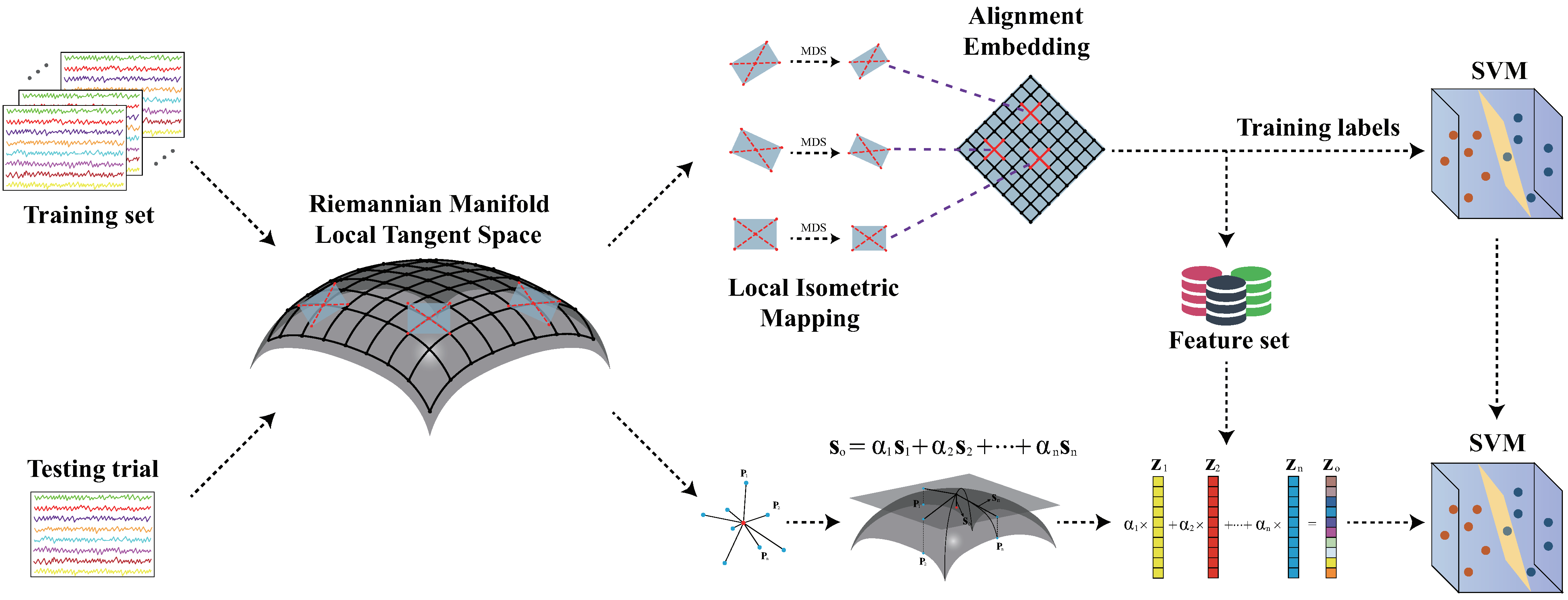
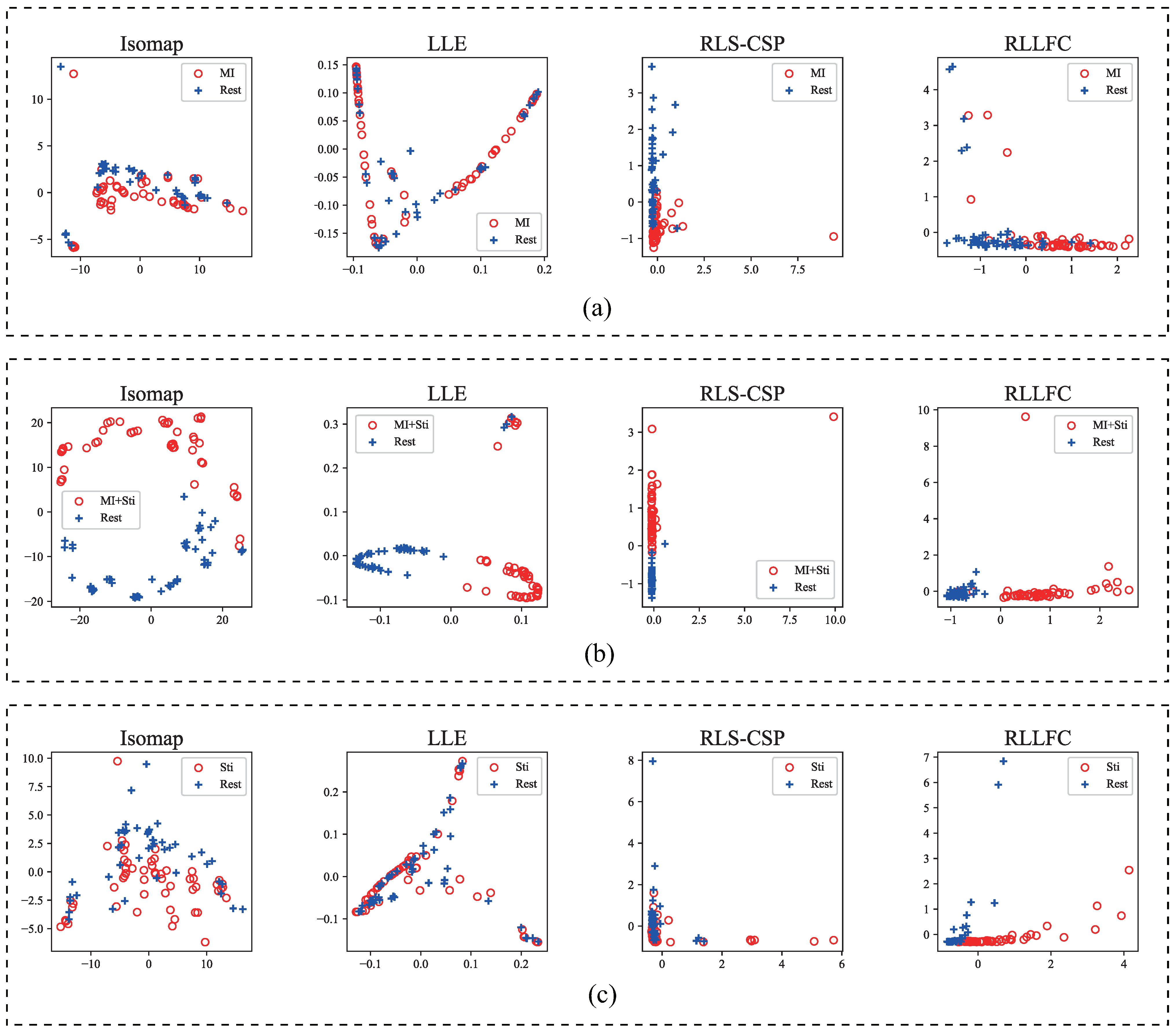
Although many efficient unsupervised basis learning and weight calculation methods have been proposed to quickly represent the testing trial EEG with a linear weighted combination of the basis learned from the training set, most of these approaches learn the basis without considering the fact that the high-dimensional EEG signal lies in a non-Euclidean space. It should be noted that the low-dimensional feature basis can be extended as a Euclidean space while the original EEG signal space is a non-Euclidean space. Therefore, the fundamental challenge in feature representation is to ensure that the learned basis maximally preserves the real relationship between EEG samples in a non-Euclidean space. In view of the shortcomings of the feature representation problem, in this study, a novel decoding method based on the Riemannian local linear feature construct (RLLFC) was designed to improve the performance of lower-limb rehabilitation BCI systems. In the proposed RLLFC method, the Riemannian geodesic distance is used to characterize the relationship between EEG samples, based on the assumption that the covariance matrices of the EEG signal lie on a differential Riemannian manifold [24]. The basis learned from RLLFC can best maintain the geodesic distance between the covariance matrices of EEG samples using a local isometric mapping. Many similar methods have been proposed to decode EEG signals in BCI systems. 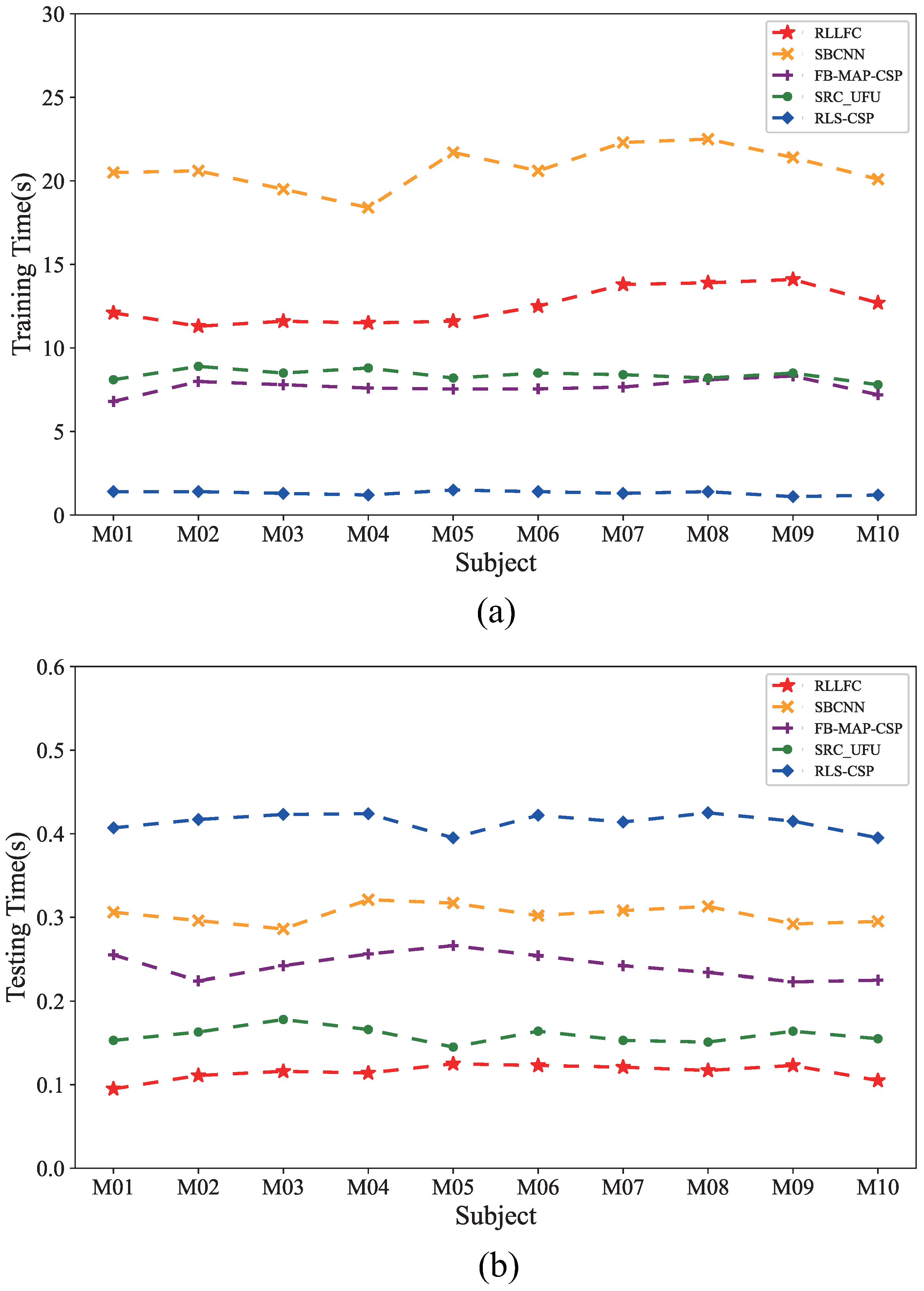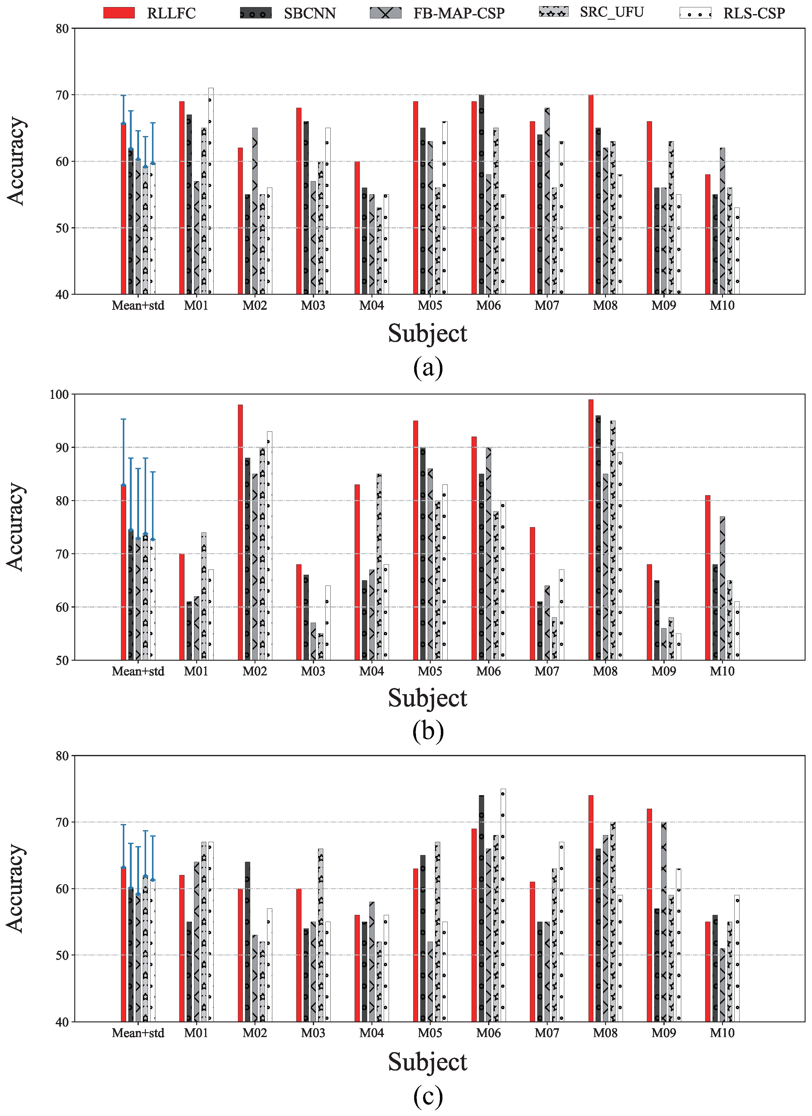In [25], a simplified Bayesian convolutional neural network (SBCNN) was proposed to decode the P300 signal in a BCI game by minimizing the Kullback–Leibler divergence between the approximate and real weight distributions. In [26], an unsupervised adaptive sparse representation-based classification (SRC_UFC) was designed to identify EEG signals by updating the basis set with new testing samples. In [27], the filter bank maximum a posteriori common spatial pattern (FB-MAP-CSP) was proposed to classify multiple MI tasks by finding the axes along which the two conditions are jointly de-correlated. In [28], recursive least squares updates of the CSP filter coefficients (RLS-CSP) was designed to recognize MI EEG signals by updating the spatial filter coefficients with new testing samples. Most of these studies have obtained excellent results in BCI applications. However, these methods ignore the fact that the covariance matrix lies on a Riemannian manifold, as well as the structural relationship between samples. The RLLFC algorithm can learn the local geometry and global structure of a Riemannian manifold by preserving the real Riemannian distance. Furthermore, it preserves the structural information of the covariance matrix. The major contributions of this study are threefold:

• A novel basis learning and representation method called RLLFC is proposed to improve the performance of decoding in MI-BCI systems. Compared with the previous methods, the RLLFC method can preserve the distance between EEG samples and the basis by using the Riemannian geometric distance to measure the EEG samples. Previous methods cannot use the geodesic distance information to learn the basis from EEG samples, owing to the unknown manifold of EEG samples.
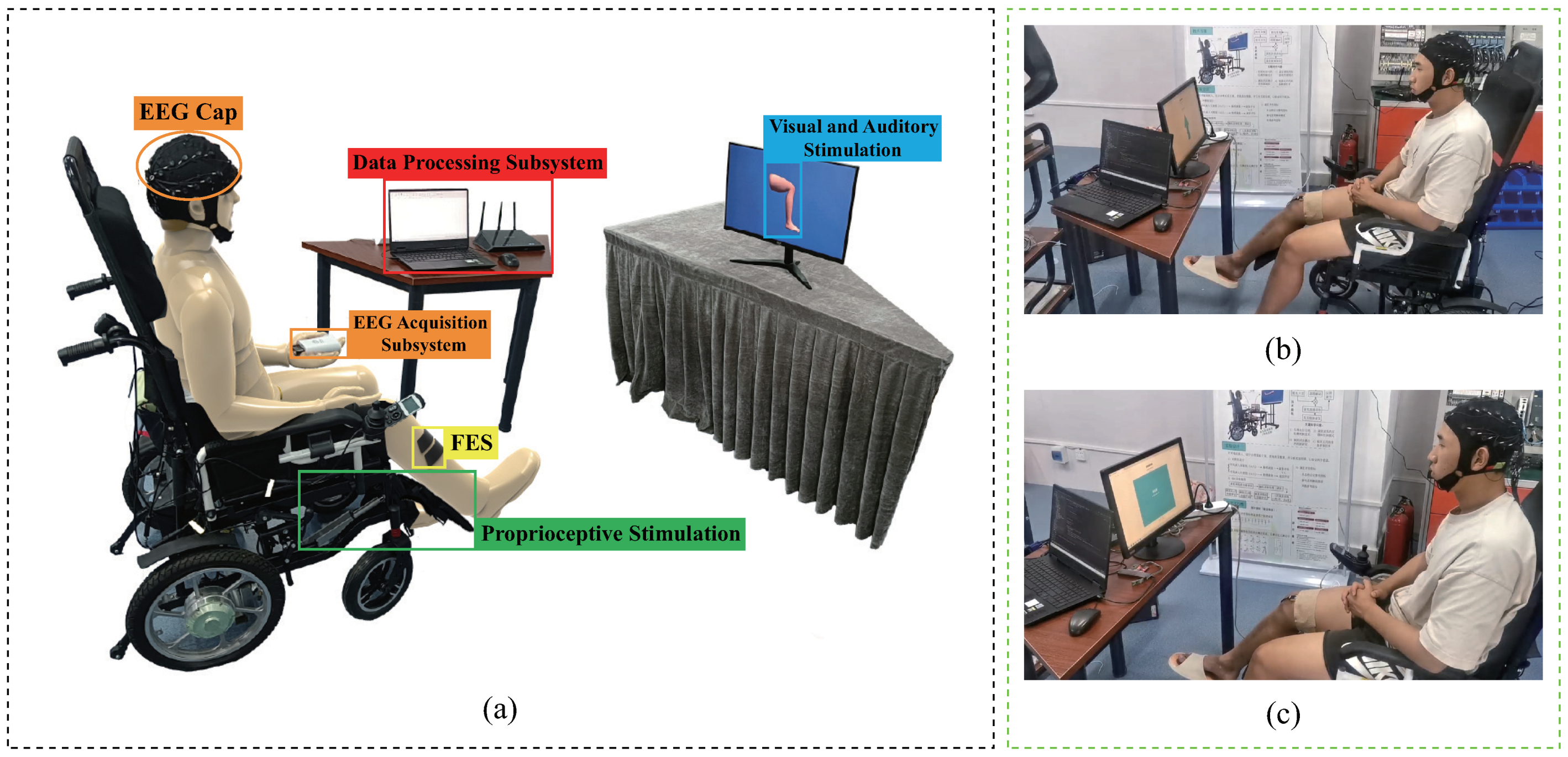
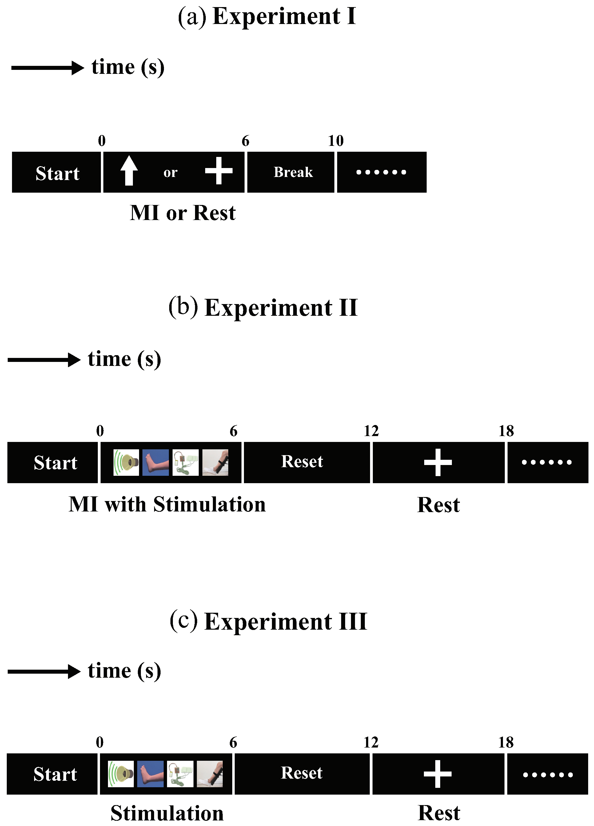
• A novel lower-limb MI-BCI system that combines visual stimulation, auditory stimulation, functional electrical stimulation (FES), and proprioceptive stimulation was designed to assist patients in lower-limb rehabilitation training.
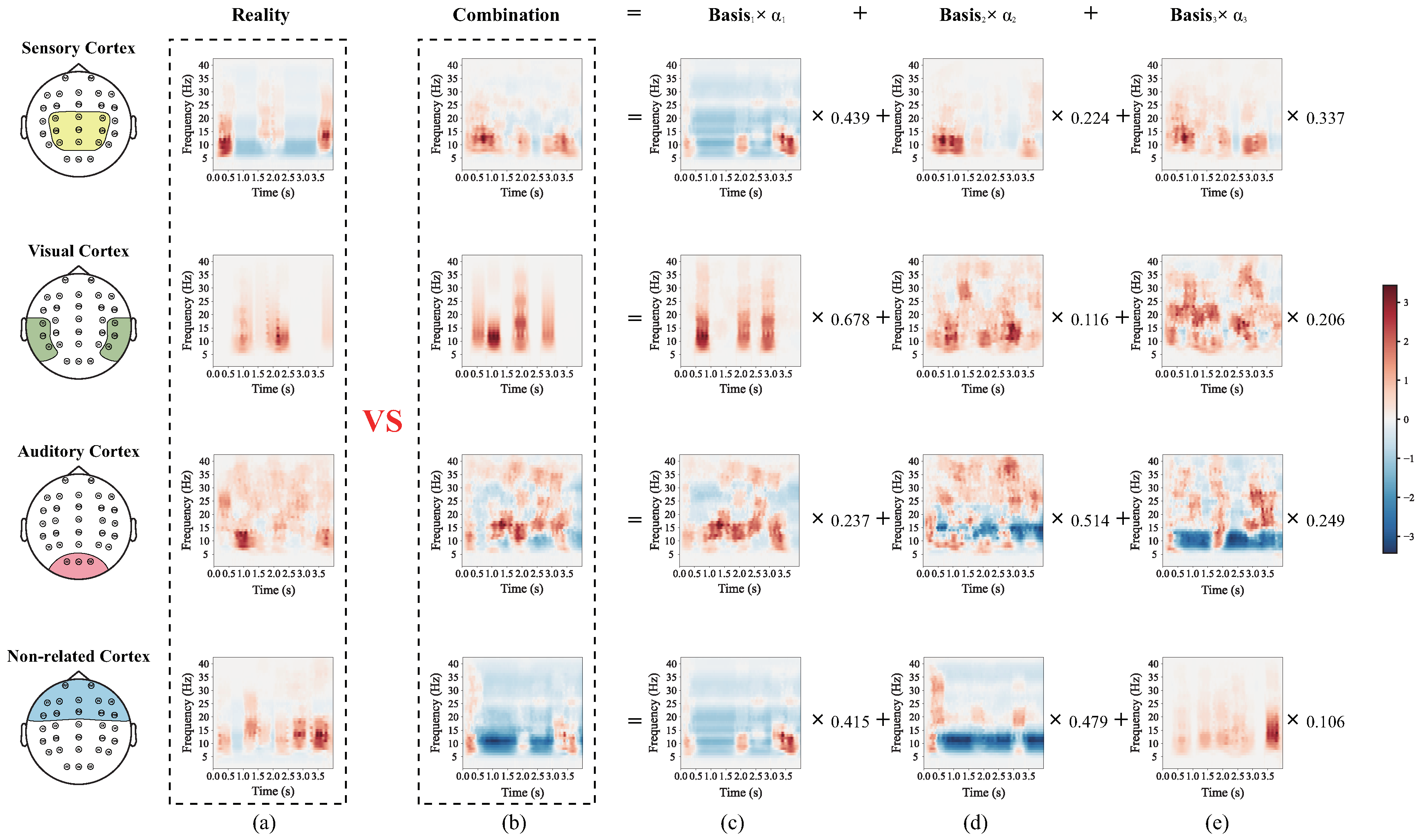
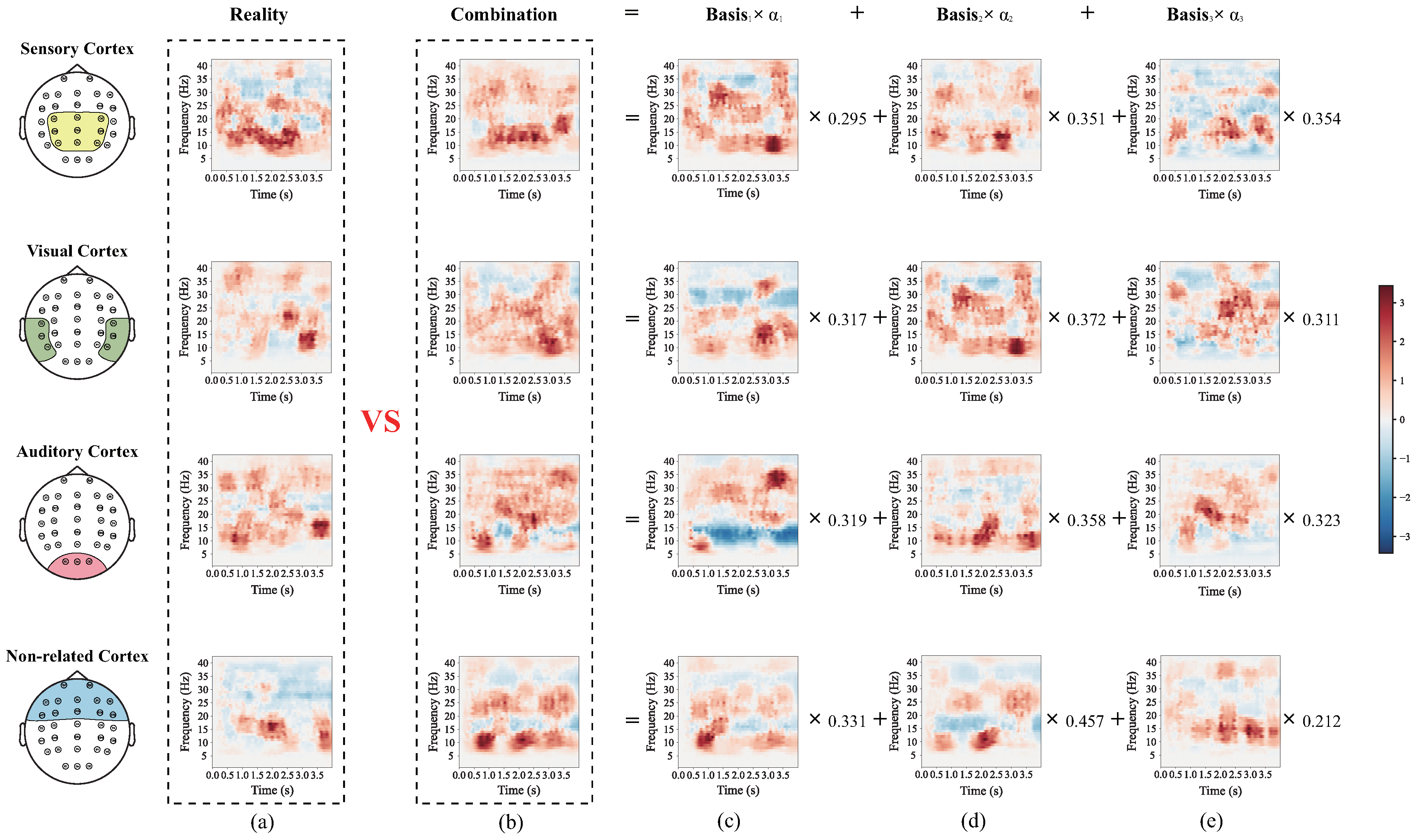
• The proposed RLLFC algorithm and BCI system can reveal the cortical activation of lower-limb motor imagery under different visual, auditory, FES, and proprioceptive stimuli, as supported by experimental results. This can provide data support for improving the performance of lower-limb rehabilitation training.

The remainder of this paper is organized as follows. In Section 2, the experimental setup and EEG decoding process are described. Section 3 provides the extensive experimental results and analysis to demonstrate the effectiveness of the proposed system. Finally, some conclusions are presented in Section 4.

2. Materials and Methods

2.1. Proposed BCI System and Experiment

Hardware structure of proposed system: As shown in Figure 1a, the hardware structure of the lower-limb MI-BCI system mainly consisted of an EEG acquisition subsystem, multimodal stimulation subsystem, and a data processing subsystem. The EEG acquisition subsystem included an EEG cap and a 30-channel active Bio-Signal EEG amplifier (Poseidon, Jiangsu, China). Electrodes were placed on the scalp at locations overlying the motor cortices. The Pz electrode was used for positioning according to the specifications of the International 10-20 Electrode System. The ground electrode was placed on AFz and the reference electrode was placed on the left earlobe. All impedances were maintained at below 20 k$\mathsf{\Omega }$ at the onset of each session. The sampling rate was set to 250 Hz. The multimodal stimulation subsystem included visual, auditory, FES, and proprioceptive stimulation. The visual stimulation consisted of a video of the lower limbs laid down or being raised while the participant performed lower-limb movement imagery. The auditory stimulation was a notification sound of “Please raise your legs”. The proprioceptive stimulation consisted of a single-degree-of-freedom mechatronic device installed on a wheelchair. The FES included two pairs of self-adhesive surface electrodes fitted onto the right leg of the participant.

Experiment: Twenty able-bodied volunteers (aged 21 ± 3 years, 8 female) participated in the proposed lower-limb motor imagery BCI system. Ethical approval was obtained from the Hainan University Ethics Committee. All of the participants provided written informed consent. We designed experiments using two control group and an experimental group for fair comparison. The group involved in the lower-limb motor imagery experiment and stimulation experiment were regarded as the control group, where that in the lower-limb motor imagery experiment with multimodal stimulation (visual, auditory, FES, and proprioceptive) was the experimental group.

(1)

Experiment I: Lower-limb motor imagery experiment. The structure of each trial is illustrated in Figure 2a. After the beginning of the experiment, a cue in the form of an arrow pointing up or a cross appeared and remained on the screen for 0–6 s. During the tasks, an upward arrow was set as a cue to prompt motor imagery, while a cross was shown as a cue to rest. The participants were instructed to begin imagining the leg movement until the arrow disappeared from the screen. There a 4 s break between tasks. A block consists of 50 trials, 25 for each of the two cues. Each participant completed three blocks, yielding a total of 150 trials.

(2)

Experiment II: Lower-limb motor imagery experiment with multimodal stimulation. The structure of each trial is illustrated in Figure 2b. From to 0–6 s, four types of stimulation were provided during motor imagery: visual, auditory, FES, and proprioceptive. The visual stimulation was a video of leg-raising; the auditory stimulation was an alert tone. FES was performed using surface electrodes, and the proprioceptive stimulation was an electric lift pedal that can raise a participant’s right leg. The participant performed motor imagery of leg raising during the stimulation period until stimulations stopped. At the end of motor imagery, the pedal returned to the starting position from 6 to 12 s. Next, a cross cue appeared and remained on the screen from 12 to 18 s to allow the participant to rest. The blocks of 50 trials comprised 25 trials for each cue. Each participant completed three blocks, for a total of 150 trials.

(3)

Experiment III: Multimodal stimulation experiment. The structure of each trial is illustrated in Figure 2c. From to 0–6 s, four types of stimulation were provided subject. The subject maintained resting state during the stimulation period until stimulations stopped. At the end of stimulations, the pedal returned to the starting position from 6 to 12 s. Next, a cross cue appeared and remained on the screen from 12 to 18 s to allow the participant to rest. The blocks of 50 trials comprised 25 trials for each cue. Each participant completed three blocks, 150 trials were conducted.

2.2. Riemannian Local Linear Feature Construction Algorithm

In this section, an RLLFC algorithm is proposed for decoding of motor imagery EEG signals based on a Riemannian manifold. As shown in Figure 3, the RLLFC algorithm consists of unsupervised basis learning and representation weight calculation.

2.2.1. Basis Learning with Local Isometric Mapping

Denoting the N-channel EEG signal with L sampled points as

$$\mathbf{X}\left(t\right)=[\mathbf{x}\left(t\right),\dots ,\mathbf{x}(t+L-1)]\in {\mathbb{R}}^{N\times L},$$

(1)

the spatial covariance matrix of $\mathbf{X}\left(t\right)$ is defined as

$$\mathbf{P}=\frac{1}{L-1}\mathbf{X}\left(t\right){\mathbf{X}}^T\left(t\right).$$

(2)

The space of spatial covariance matrices with symmetric positive definite (SPD) forms lies on a differentiable Riemannian manifold $\mathcal{M}$ [29]. The Riemannian geodesic distance between two spatial covariance matrices ${\mathbf{P}}_1,{\mathbf{P}}_2\in \mathcal{M}\left(N\right)$ is defined as

$${\delta }_R\left({\mathbf{P}}_1,{\mathbf{P}}_2\right)={∥log\left({\mathbf{P}}_1^{-1}{\mathbf{P}}_2\right)∥}_F={\left[\sum _{i=1}^N{log}^2{\beta }_i\right]}^{\frac{1}{2}},$$

(3)

where ${\parallel ·\parallel }_F$ is the Frobenius norm of a matrix and ${\beta }_i$ is the i-th real eigenvalue of ${\mathbf{P}}_1^{-1}{\mathbf{P}}_2$.

After characterizing the relationships between EEG samples in the Riemannian manifold, we learned the basis from the training dataset using an unsupervised Riemannian manifold learning method. More specifically, we first designed a local isometric mapping to preserve the real relationships between the EEG samples as effectively as possible from the Riemannian manifold to a low-dimensional subspace. For a data point $\mathbf{P}$ in the Riemannian manifold, we selected the k-nearest neighbor of $\mathbf{P}$ according to the Riemannian geodesic distance. The local tangent space $\mathcal{T}$ is defined as the tangent space at $\mathbf{P}$, and all of its neighboring points are mapped into tangent space,

$$\begin{array}{ccc}\hfill & \mathcal{T}=\hfill & \hfill \left\{{\mathbf{s}}_i=\mathrm{upper}\left({\mathbf{P}}^{-\frac{1}{2}}Lo{g}_{\mathbf{P}}\left({\mathbf{P}}_i\right){\mathbf{P}}^{-\frac{1}{2}}\right),{\mathbf{P}}_i\in neighbor\right\}\end{array}$$

(4)

where the upper (.) operator is used to retain and vectorize the upper triangular part of the matrix. The logarithmic mapping operator is denoted by $Lo{g}_{\mathbf{P}}\left({\mathbf{P}}_i\right)={\mathbf{P}}^{\frac{1}{2}}log\left({\mathbf{P}}^{-\frac{1}{2}}{\mathbf{P}}_i{\mathbf{P}}^{-\frac{1}{2}}\right){\mathbf{P}}^{\frac{1}{2}}$. The local tangent space represents the local structure of the data in the Riemannian manifold.

Multidimensional scaling (MDS) is a widely used approach to dimensionality reduction. It projects data objects onto a low dimensional space while preserving the original distances among them as much as possible. Local Isometric Mapping is based on MDS. Isometric mapping was applied in each local tangent space to reduce the dimensions and preserve the structure. This can be achieved using the following optimization problem:  

$$min{∥\psi \left(\mathbf{D}\right)-\psi \left({\mathbf{D}}^{\prime }\right)∥}_F^2,$$

(5)

where $\mathbf{D}$ is the distance matrix of points ${\mathbf{s}}_i$, ${\mathbf{s}}_j$ on the local tangent space $\mathcal{T}$ with ${\left(\mathbf{D}\right)}_{ij}={∥{\mathbf{s}}_i-{\mathbf{s}}_j∥}_F={\delta }_R\left({\mathbf{P}}_i,{\mathbf{P}}_j\right)$. ${\mathbf{D}}^{\prime }$ is the distance matrix of points ${\mathbf{y}}_i$ in a low-dimensional subspace. $\psi (·)$ denotes an operator from distance matrix to inner product matrix. The optimization problem in (5) can be solved by eigenvalue decomposition:

$$\mathbf{Y}={\lambda }^{1/2}{\mathbf{K}}^T,$$

(6)

where $\lambda$ consists of the d largest eigenvalues of $\psi \left(\mathbf{D}\right)$ and $\mathbf{K}$ consists of the d eigenvectors corresponding to the d largest eigenvalues [30].

Finally, we utilized reconstruction processing in locally linear embedding to align all subspaces of the local tangent space to global coordinates [31]. The weights $w_{ij}$ that best linearly fit point ${\mathbf{y}}_i$ between its neighbors can be learned by

$$\underset{{\mathbf{w}}_i}{min}{∥{\mathbf{y}}_i-\sum _j{w}_{ij}{\mathbf{y}}_j∥}_F^2.$$

(7)

Furthermore, the matrix $\mathbf{W}$ represented structural information of all local neighborhoods, the global coordinates $\mathbf{Z}$ can be learned from each tangent subspace by keeping the weight $w_{ij}$:

$$\underset{\mathbf{Z}}{min}\sum _i{∥{\mathbf{z}}_i-\sum _j{w}_{ij}{\mathbf{z}}_j∥}_F^2.$$

(8)

Equation (8) can be converted to

$$\underset{\mathbf{Z}}{min}\mathbf{Z}(\mathbf{I}-\mathbf{W}){(\mathbf{I}-\mathbf{W})}^T{\mathbf{Z}}^T.$$

(9)

Define $\mathbf{M}=(\mathbf{I}-\mathbf{W}){(\mathbf{I}-\mathbf{W})}^T$, the global coordinates $\mathbf{Z}$ can be obtained by solving the null space of the $\mathbf{M}$. And ${\mathbf{z}}_i$ is the i-th row of matrix $\mathbf{Z}$. Thus, matrix $\mathbf{Z}$ is the basis learned from the training dataset.

2.2.2. Representation Weight Calculation

For an testing EEG trial ${\mathbf{X}}_o\left(t\right)$, we expect to find a linear combination of bases ${\mathbf{z}}_i$ learned from the training dataset to best represent the features of ${\mathbf{X}}_o\left(t\right)$ as follows:

$${\mathbf{z}}_o=\sum _{i=1}^k{\alpha }_i{\mathbf{z}}_i.$$

(10)

To this end, the key problem is the calculation of representation weight ${\alpha }_i$. Inspired by the weight calculation in the locally linear embedding method, we first selected the $k_o$-nearest neighbors of ${\mathbf{P}}_o$ based on the Riemannian geodesic distance, where ${\mathbf{P}}_o$ is the spatial covariance matrix of ${\mathbf{X}}_o\left(t\right)$. Furthermore, ${\mathbf{P}}_o$ and its neighbors were mapped into the local tangent space, and the Riemannian mean of ${\mathbf{P}}_o$ and its neighbors was regarded as a tangent point. The representation weight ${\alpha }_i$ can be learned using the following optimization:

$$\underset{{\alpha }_i}{min}{∥{\mathbf{s}}_o-\sum _{i=1}^k{\alpha }_i{\mathbf{s}}_i∥}_F^2,$$

(11)

where ${\mathbf{s}}_o$ is the tangent vector of ${\mathbf{P}}_o$ and ${\mathbf{s}}_i$ is the tangent vector of i-neighbor. Support vector machine (SVM) is a supervised machine learning algorithm that develops an optimal hyperplane that allows classification of input data. In the case of the SVM, a SVM with radial basis functions as kernels was used for classification. The pseudocode for RLLFC is provided in Algorithm 1.

Algorithm 1: Riemannian local linear feature construction (RLLFC)

Input:  Training datasets ${\mathbf{X}}_{tr}$ with label ${\mathbf{l}}_{tr}$ and testing EEG trial ${\mathbf{X}}_o\left(t\right)$; Output:  Label $l_o$ of testing EEG trial ${\mathbf{X}}_o\left(t\right)$; 1: Compute a set of covariance matrices ${\mathbf{P}}_{tr}$ of ${\mathbf{X}}_{tr}$; 2: for 1=1: 1:($|{\mathbf{P}}_{tr}|$), $\mathbf{do}$; 3:      Construct local tangent space ${\mathcal{T}}_i$ for ${\mathbf{P}}_i$ using (4); 4:      Calculate ${\mathbf{D}}_i$ for local tangent space ${\mathcal{T}}_i$; 5:      Obtain low-dimensional subspace ${\mathbf{Y}}_i$ using (6); 6:      Compute weight ${\mathbf{w}}_i$ using (7); 7: end for 8: Reconstruct the global coordinates $\mathbf{Z}$ using (8); 9: Utilize $\mathbf{Z}$ and ${\mathbf{l}}_{tr}$ to train SVM classifier; 10: Compute covariance matrices ${\mathbf{P}}_o$ of ${\mathbf{X}}_o$; 11: Map ${\mathbf{P}}_o$ and its neighbors into local tangent space; 12: Learn weights $[{\alpha }_1,{\alpha }_2,...,{\alpha }_k]$ using (10); 13: Construct feature ${\mathbf{z}}_o$ based on $[{\alpha }_1,{\alpha }_2,...,{\alpha }_k]$ using (9); 14: Predict ${\mathbf{z}}_o$ using the SVM classifier;

3. Results and Discussion

3.1. Data and Algorithm Description

Data description: Three datasets were used to demonstrate the effectiveness of the proposed method:

(1)

The in-house dataset was recorded from ten subjects (M01–M10) who performed experiment I. The recorded signals consisted of 30 EEG channels. For each subject, there were two types of EEG signals, the lower-limb motor imagery and rest conditions. The training set and testing set were randomly divided at a quantity ratio of 2:1. In total, 100 samples for the training phase, 50 samples for the testing phase.

(2)

The in-house dataset was recorded from twenty subjects (M01–M20) who performed experiment II. The recorded signals consisted of 30 EEG channels. For each subject, there were two types of EEG signals, the lower-limb motor imagery with multimodal stimulation and rest conditions. The training set and testing set were randomly divided at a quantity ratio of 2:1. Thus, the overall number of training/testing trials for each subject was 100/50.

(3)

The in-house dataset was recorded from twenty subjects (M01–M10) who performed experiment III. The recorded signals consisted of 30 EEG channels. For each subject, there were two types of EEG signals, the multimodal stimulation and rest conditions. The training set and testing set were randomly divided at a quantity ratio of 2:1. Broadly, the training set comprised 100 trials, and the testing set comprised 50 trials.

Algorithms evaluated: To evaluate the performance, four competing algorithms for EEG decoding were used as follows:

(1)

SBCNN: a simplified Bayesian convolutional neural network (SBCNN) was proposed to decode the EEG signal by minimizing the Kullback–Leibler divergence between the approximate and real distributions [25].

(2)

FB-MAP-CSP: this approach decomposes EEG signals into multiple-frequency band-pass bands and uses the MAP-CSP algorithm to extract the features at each sub-band separately, with linear discriminant analysis performing classification [27].

(3)

SRC_UFU: An EEG classification algorithm based on a sparse representation. This method was designed to identify the EEG signals by updating the basis set with new testing samples [26].

(4)

RLS-CSP: a fast generalized eigen-decomposition method that updates the filter coefficients using recursive least squares [28].

3.2. Parameter Setting by 5-Fold Cross-Validation

In the RLLFC algorithm, the three parameters k, d, and $k_o$ must be calculated before test processing. In our study, the parameters were learned through a 5-fold cross-validation scheme, in which the training data were divided into five parts; one was kept as the validation set, and the other four were used as the training set. Considering the two-class classification problem of an in-house BCI, for simplicity, the classification accuracy was used as a performance measure for the in-house dataset. Figure 4 shows the 5-fold cross-validation classification accuracies of the best parameter combinations for the in-house dataset corresponding to experiments I, II and III. For each subject, the parameter k was set as $[19,11,15,17,9,15,19,11,15,13]$ in experiment I, $[17,19,17,19,19,15,17,11,13,19,15,13,15,$$17,19,19,17,15,13,15]$ in experiment II, and $[19,17,11,11,19,17,13,19,19,19]$ in experiment III. The parameters d and $k_o$ were set as $[8,6,6,6,4,2,4,6,4,4]$ and $[3,9,7,7,5,3,9,9,3,3]$, respectively, in experiment I; $[4,6,6,8,8,6,8,8,8,8,6,6,8,8,8,6,8,6,8,8]$ and $[3,9,7,7,3,7,9,3,$$9,7,9,9,7,5,7,9,5,3,7,9]$, respectively, in experiment II; and $[6,8,4,6,6,8,8,6,8,4]$ and $[7,7,9,7,$$9,5,7,3,7,9]$, respectively, in experiment III. In the SVM, the penalty parameter C set to 1.0 and the kernel coefficient $\gamma$ set to 0.1.

Furthermore, to demonstrate the generalization capacity of the proposed model, we compared the proposed algorithm with four other competing classification algorithms, that is, SBCNN, FB-MAP-CSP, SRC_UFU, and RLS-CSP, using 5-fold cross-validation. As shown in Figure 4, the RLLFC method outperformed the competing methods for all subjects and had a higher accuracy and lower standard deviation than those of the other competing methods. This indicates that our RFFLC model is more stable than the other four methods. In addition, we provide a significance analysis of the cross-validation results in Figure 4. From the paired t-test results in

Table 1. t-test results for the proposed method versus competing method via 5-fold cross-validation (M01–M10).

Paired t-Test	In-House Dataset I	In-House Dataset II	In-House Dataset III
	$p$-Value	$p$-Value	$p$-Value
RLLFC vs. SBCNN	†	$††$	∼
RLLFC vs. FB-MAP-CSP	*	$††$	*
RLLFC vs. SRC_UFU	$††$	†	∼
RLLFC vs. RLS-CSP	†	$††$	∼

Note: ∼ nonsignificant, * $p\le$ 0.05, † $p\le$ 0.005, $††$$p\le$ 0.001

, it is clear that the differences between RLLFC and other competing methods are statistically significant, supporting the superiority of RLLFC’s generalization capacity.

3.3. Classification Performance of RFFLC

Table 2. Results of experiment I (MI) for all studied algorithms (%).

Method	Mean	Subject
	Accuracy	M01	M02	M03	M04	M05	M06	M07	M08	M09	M10
RLLFC	74.8	90	74	68	80	92	78	64	80	64	58
SBCNN	68.8	82	66	64	78	76	66	60	64	70	62
FB-MAP-CSP	65.4	72	70	70	64	72	64	58	70	54	60
SRC_UFU	64.8	78	62	66	64	68	60	66	62	66	56
RLS-CSP	66.6	76	66	72	66	82	58	60	62	58	66

and

Table 3. Results of experiment II (MI with stimulation) for all studied algorithms (%).

Method	Mean	Subject
	Accuracy	M01	M02	M03	M04	M05	M06	M07	M08	M09	M10
RLLFC	87.2	84	96	80	78	90	96	74	98	98	78
SBCNN	78.8	80	90	68	80	86	86	64	84	88	62
FB-MAP-CSP	76.6	74	86	66	74	78	80	68	78	86	76
SRC_UFU	80.2	72	82	78	76	82	84	76	90	92	70
RLS-CSP	78.2	82	80	72	64	80	92	66	94	84	68

present the classification accuracies of the RLLFC algorithm for lower-limb movement imagery with and without stimulation, respectively, corresponding to experiments I and II. For a fair comparison, we also compared RLLFC with the SBCNN, FB-MAP-CSP, SRC_UFU, and RLS-CSP algorithms for decoding. As shown in Table 2, the proposed RLLFC achieved a mean accuracy of 74.8% for experiment I, which was higher than those of SBCNN, FB-MAP-CSP, SRC_UFU, and RLS-CSP by 6.0%, 9.4%, 10.0%, and 8.2%, respectively. Furthermore, as shown in Table 3, the proposed RLLFC achieved a mean accuracy of 87.2% for experiment II, which was higher than those of SBCNN, FB-MAP-CSP, SRC_UFU, and RLS-CSP by 8.4%, 10.6%, 7.0%, and 9.0%, respectively. Comparing Table 2, Table 3 and

Table 4. Results of experiment III (stimulation) for all studied algorithms (%).

Method	Mean	Subject
	Accuracy	M01	M02	M03	M04	M05	M06	M07	M08	M09	M10
RLLFC	71.4	82	70	78	64	70	70	66	84	66	64
SBCNN	68.8	70	74	68	60	80	72	64	68	70	62
FB-MAP-CSP	67.2	78	62	72	68	62	64	60	72	64	70
SRC_UFU	69.4	80	78	68	70	66	62	62	68	72	68
RLS-CSP	70.2	74	64	66	74	78	68	68	78	60	72

, the accuracies of movement imagery with stimulation are still higher than the accuracies of movement imagery and stimulation experiment. It can be inferred that multimodal stimulation can help improve motor imagery ability to obtain a high classification performance. To demonstrate model performance, data were collected from subjects (M11–M20); as shown in

Table 5. Results of experiment II (MI with stimulation) for all studied algorithms (%).

Method	Mean	Subject
	Accuracy	M11	M12	M13	M14	M15	M16	M17	M18	M19	M20
RLLFC	88.4	86	94	80	96	70	92	92	88	96	90
SBCNN	81.6	76	88	78	82	76	80	88	86	86	76
FB-MAP-CSP	78.4	80	78	70	90	64	82	84	70	82	84
SRC_UFU	80.8	84	82	72	84	72	88	80	78	90	78
RLS-CSP	80.2	78	90	84	94	64	84	74	72	82	80

, the proposed RLLFC achieved a mean accuracy of 88.4% for experiment II. It was observed from

Table 6. Recall of each class for the proposed method in the test (M01–M10) (%).

Class	Mean	Subject
	Recall	M01	M02	M03	M04	M05	M06	M07	M08	M09	M10
True of In-house dataset I	75.6	92	80	72	76	88	80	68	76	60	64
False of In-house dataset I	74.0	88	68	64	84	96	76	60	84	68	52
True of In-house dataset II	87.6	80	96	76	84	88	96	76	100	96	84
False of In-house dataset II	86.8	88	96	84	72	92	96	72	96	100	72
True of In-house dataset III	70.4	80	76	72	60	68	76	60	84	60	68
False of In-house dataset III	72.4	84	64	84	68	72	64	72	84	72	60

that the recall of two classes are close, and there is no bias towards any of them. The t-test analysis of Table 2, Table 3 and Table 4 are shown in

Table 7. t-test results for the proposed method versus competing method in the test (M01–M10).

Paired t-Test	In-House Dataset I	In-House Dataset II	In-House Dataset III
	$p$-Value	$p$-Value	$p$-Value
RLLFC vs. SBCNN	*	$††$	∼
RLLFC vs. FB-MAP-CSP	†	$††$	*
RLLFC vs. SRC_UFU	**	†	∼
RLLFC vs. RLS-CSP	*	$††$	∼

Note: ∼ nonsignificant, * $p\le$ 0.05, ** $p\le$ 0.01, † $p\le$ 0.005, $††$$p\le$ 0.001

; it can be seen that the differences between RLLFC and other competing methods are statistically significant. Based on the results of the experiments, it was concluded that the proposed RLLFC has better decoding performance than the other state-of-the-art algorithms.

To demonstrate the efficiency of the testing processing of the RLLFC algorithm, we also compared the computational loads of the proposed algorithm with those of the competing algorithms using Python 3.6 and a 3.2 GHz CPU. Figure 5 show the training and testing times of each algorithm. The training time denotes the computational load of the model training on the training dataset, whereas the test time is the mean computational load of the processing of 50 trials for classification. As shown in Figure 5, the training times of RFFLC were shorter than those of SBCNN for the in-house datasets and longer than those of FB-MAP-CSP and RLS-CSP, because calculation of the Riemannian distance requires more time for high-dimensional manifolds. However, the test time of RFFLC was the shortest in-house datasets. The RFFLC method takes a mean time of 0.13 s for decoding of a single trial. Therefore, considering both time-consumption and performance for in-house datasets, RFFLC presents a comparable advantage over the other options.

3.4. Classification Performance Supporting Analysis

To support the high classification performance of RLLFC in the previous results, we analyzed the performance of basis learning and representation weight calculation in the proposed RLLFC algorithm. For basis learning, we designed an unsupervised dimensionality reduction method called local isometric mapping to obtain low-dimensional features. The corresponding feature distribution of the two-dimensional embedding of the EEG signal learned by the RLLFC algorithm is presented in Figure 6. For a fairer comparison, we also show the two-dimensional features of three competing dimensionality reduction algorithms: Isomap, LLE, and RLS-CSP. As shown in Figure 6, the discriminative features learned by RLLFC have much higher separability than Isomap, LLE, and RLS-CSP. It can be inferred that the basis learned by RLLFC could maintain the separability of the EEG signal to support the high classification performance of RLLFC.

To demonstrate the representation effects of the RLLFC algorithm, we compared the time-frequency diagram of the EEG signal in the testing trials with the linear combination of its $k_o$-nearest neighbors from the training trials. The representation weight ${\alpha }_i$ for the linear combination was calculated using Equation (10). For intuitive visualization, the time-frequency diagram of the EEG signal was used to express the effect of the linear combination. Because the short-time Fourier transform is a linear transformation, the linear combination of the time-frequency diagram is equivalent to a linear combination of EEG signals. Figure 7 shows the time-frequency diagram of lower-limb movement imagery with and without stimulation. Comparing Figure 7a–e, it can be observed that the real time-frequency diagram of the EEG signal can be approximately expressed as a linear combination of the time-frequency diagrams of its 3-nearest neighbors weighted by the representation coefficients $[{\alpha }_1,{\alpha }_2,{\alpha }_3]$. These results prove that the representation weight learned by RLLFC can correctly characterize the relationship between the testing trial and its k-nearest neighbors, supporting the high decoding performance of this approach.

3.5. Effect of Stimulation on RLLFC

More specifically, to discuss the difference between RLLFC performed on the lower-limb movement imagery with and without stimulation, we analyzed the four time-frequencies corresponding to the mean EEG signal in four different brain cortices, that is, the sensory cortex, visual cortex, auditory cortex, and a non-related cortex. As shown in Figure 8 and Figure 9, the time-frequency approximate representation of the sensory cortex is closer to the real time frequency than those of the visual cortex, auditory cortex and non-related cortex. Moreover, the time-frequency approximate representations of the visual and auditory cortices are closer to the real time frequency than that of non-related cortex. Note that we have proven that RFFLC is an efficient feature representation method for lower-limb motor imagery and can accurately reconstruct features of lower-limb motor imagery EEG. The results in Figure 8 show that the sensory cortex area is mainly involved in pure motor imagery, whereas the visual and auditory cortices involved little pure motor imagery. In addition, by combining the time-frequency diagrams of the sensory cortex in Figure 8 and Figure 9, it is observed that the rhythm range related to MI in Figure 9 is larger than that in Figure 8. The same result was observed in the visual and auditory cortices. This is because the neurons in the sensory, visual, and auditory cortices were stimulated and reinforced in experiment II, which included FES, proprioceptive stimulation, visual stimulation, and auditory stimulation. These results prove that stimulation can increase the cortical activation of the motor cortical areas.

4. Conclusions

In this study, a novel lower-limb BCI system combining visual stimulation, auditory stimulation, FES, and proprioceptive stimulation was designed to assist patients in lower-limb rehabilitation training. Furthermore, the RLLFC algorithm was proposed to improve the performance of decoding by using unsupervised basis learning and representation weight calculation in a motor imagery BCI system. Compared with other competing methods, the proposed RLLFC method can learn low-dimensional features and correctly characterize the relationship between an testing trial and its k-nearest neighbors. The experimental results demonstrate the effectiveness of the proposed system. However, the training process in RLLFC incurs a very large computational load because of the Riemannian distance calculation. Future work will modify the proposed RLLFC used in the training process.

References

1. Jin, J.; Xiao, R.; Daly, I.; Miao, Y.; Wang, X.; Cichocki, A. Internal Feature Selection Method of CSP Based on L1-Norm and Dempster–Shafer Theory. IEEE Trans. Neural Networks Learn. Syst. 2021, 32, 4814–4825. [Google Scholar] [CrossRef] [PubMed]
2. Abiri, R.; Borhani, S.; Sellers, E.W.; Jiang, Y.; Zhao, X. A comprehensive review of EEG-based brain–computer interface paradigms. J. Neural Eng. 2019, 16, 011001. [Google Scholar] [PubMed]
3. Sun, H.; Jin, J.; Xu, R.; Cichocki, A. Feature selection combining filter and wrapper methods for motor-imagery based brain–computer interfaces. Int. J. Neural Syst. 2021, 31, 2150040. [Google Scholar] [CrossRef]
4. Bulárka, S.; Gontean, A. Brain-computer interface review. In Proceedings of the 2016 12th IEEE International Symposium on Electronics and Telecommunications (ISETC), Timisoara, Romania, 27–28 October 2016; IEEE: Piscataway, NJ, USA, 2016; pp. 219–222. [Google Scholar]
5. Bobrova, E.; Reshetnikova, V.; Frolov, A.; Gerasimenko, Y.P. Use of imaginary lower limb movements to control brain–computer interface systems. Neurosci. Behav. Physiol. 2020, 50, 585–592. [Google Scholar] [CrossRef]
6. Delisle-Rodriguez, D.; Cardoso, V.; Gurve, D.; Loterio, F.; Romero-Laiseca, M.A.; Krishnan, S.; Bastos-Filho, T. System based on subject-specific bands to recognize pedaling motor imagery: Towards a BCI for lower-limb rehabilitation. J. Neural Eng. 2019, 16, 056005. [Google Scholar] [PubMed]
7. Wang, Z.; Zhou, Y.; Chen, L.; Gu, B.; Liu, S.; Xu, M.; Qi, H.; He, F.; Ming, D. A BCI based visual-haptic neurofeedback training improves cortical activations and classification performance during motor imagery. J. Neural Eng. 2019, 16, 066012. [Google Scholar] [CrossRef]
8. Shen, F.; Deng, H.; Yu, L.; Cai, F. Open-source mobile multispectral imaging system and its applications in biological sample sensing. Spectrochim. Acta Part Mol. Biomol. Spectrosc. 2022, 280, 121504. [Google Scholar] [CrossRef]
9. Zhang, X.; Guo, Y.; Gao, B.; Long, J. Alpha frequency intervention by electrical stimulation to improve performance in mu-based BCI. IEEE Trans. Neural Syst. Rehabil. Eng. 2020, 28, 1262–1270. [Google Scholar] [CrossRef]
10. Zhang, L.; Chen, L.; Wang, Z.; Zhang, X.; Liu, X.; Ming, D. Enhancing Visual-Guided Motor Imagery Performance via Sensory Threshold Somatosensory Electrical Stimulation Training. IEEE Trans. Biomed. Eng. 2022, 70, 756–765. [Google Scholar] [CrossRef]
11. Zhang, W.; Song, A.; Zeng, H.; Xu, B.; Miao, M. Closed-loop phase-dependent vibration stimulation improves motor imagery-based brain-computer interface performance. Front. Neurosci. 2021, 15, 638638. [Google Scholar]
12. Vidaurre, C.; Murguialday, A.R.; Haufe, S.; Gómez, M.; Müller, K.R.; Nikulin, V.V. Enhancing sensorimotor BCI performance with assistive afferent activity: An online evaluation. Neuroimage 2019, 199, 375–386. [Google Scholar] [PubMed]
13. Zhong, Y.; Yao, L.; Wang, J.; Wang, Y. Tactile sensation assisted motor imagery training for enhanced BCI performance: A randomized controlled study. IEEE Trans. Biomed. Eng. 2022, 70, 694–702. [Google Scholar] [CrossRef] [PubMed]
14. Park, S.; Ha, J.; Kim, D.H.; Kim, L. Improving motor imagery-based brain-computer interface performance based on sensory stimulation training: An approach focused on poorly performing users. Front. Neurosci. 2021, 15, 732545. [Google Scholar] [CrossRef] [PubMed]
15. An, P.; Yuan, Z.; Zhao, J. Unsupervised multi-subepoch feature learning and hierarchical classification for EEG-based sleep staging. Expert Syst. Appl. 2021, 186, 115759. [Google Scholar] [CrossRef]
16. Zhuang, X.; Rozgić, V.; Crystal, M. Compact unsupervised EEG response representation for emotion recognition. In Proceedings of the IEEE-EMBS International Conference on Biomedical and Health Informatics (BHI), Valencia, Spain, 1–4 June 2014; IEEE: Piscataway, NJ, USA, 2014; pp. 736–739. [Google Scholar]
17. Al Shiam, A.; Islam, M.R.; Tanaka, T.; Molla, M.K.I. Electroencephalography based motor imagery classification using unsupervised feature selection. In Proceedings of the 2019 International Conference on Cyberworlds (CW), Kyoto, Japan, 2–4 October 2019; IEEE: Piscataway, NJ, USA, 2019; pp. 239–246. [Google Scholar]
18. Wen, T.; Zhang, Z. Deep convolution neural network and autoencoders-based unsupervised feature learning of EEG signals. IEEE Access 2018, 6, 25399–25410. [Google Scholar] [CrossRef]
19. Sun, L.; Jin, B.; Yang, H.; Tong, J.; Liu, C.; Xiong, H. Unsupervised EEG feature extraction based on echo state network. Inf. Sci. 2019, 475, 1–17. [Google Scholar]
20. Zhou, W.; Yang, Y.; Yu, Z. Discriminative dictionary learning for EEG signal classification in Brain-computer interface. In Proceedings of the 2012 12th International Conference on Control Automation Robotics & Vision (ICARCV), Guangzhou, China, 5–7 December 2012; IEEE: Piscataway, NJ, USA, 2012; pp. 1582–1585. [Google Scholar]
21. Sreeja, S.; Samanta, D.; Sarma, M. Weighted sparse representation for classification of motor imagery EEG signals. In Proceedings of the 2019 41st Annual International Conference of the IEEE Engineering in Medicine and Biology Society (EMBC), Berlin, Germany, 23–27 July 2019; IEEE: Piscataway, NJ, USA, 2019; pp. 6180–6183. [Google Scholar]
22. Kashefpoor, M.; Rabbani, H.; Barekatain, M. Supervised dictionary learning of EEG signals for mild cognitive impairment diagnosis. Biomed. Signal Process. Control. 2019, 53, 101559. [Google Scholar]
23. Gu, X.; Fan, Y.; Zhou, J.; Zhu, J. Optimized projection and fisher discriminative dictionary learning for EEG emotion recognition. Front. Psychol. 2021, 12, 705528. [Google Scholar]
24. Barachant, A.; Bonnet, S.; Congedo, M.; Jutten, C. Multiclass brain–computer interface classification by Riemannian geometry. IEEE Trans. Biomed. Eng. 2011, 59, 920–928. [Google Scholar] [CrossRef]
25. Li, M.; Li, F.; Pan, J.; Zhang, D.; Zhao, S.; Li, J.; Wang, F. The MindGomoku: An online P300 BCI game based on bayesian deep learning. Sensors 2021, 21, 1613. [Google Scholar] [CrossRef]
26. Shin, Y.; Lee, S.; Ahn, M.; Cho, H.; Jun, S.C.; Lee, H.N. Simple adaptive sparse representation based classification schemes for EEG based brain–computer interface applications. Comput. Biol. Med. 2015, 66, 29–38. [Google Scholar] [CrossRef] [PubMed]
27. Zahid, S.; Aqil, M.; Tufail, M.; Nazir, M. Online classification of multiple motor imagery tasks using filter bank based maximum-a-posteriori common spatial pattern filters. Irbm 2020, 41, 141–150. [Google Scholar] [CrossRef]
28. Jiang, Q.; Zhang, Y.; Ge, G.; Xie, Z. An adaptive csp and clustering classification for online motor imagery EEG. IEEE Access 2020, 8, 156117–156128. [Google Scholar] [CrossRef]
29. Nguyen, C.H.; Artemiadis, P. EEG feature descriptors and discriminant analysis under Riemannian Manifold perspective. Neurocomputing 2018, 275, 1871–1883. [Google Scholar]
30. Liu, Y.; Liu, Y.; Chan, K.C. Multilinear isometric embedding for visual pattern analysis. In Proceedings of the 2009 IEEE 12th International Conference on Computer Vision Workshops, ICCV Workshops, Kyoto, Japan, 27 September–4 October 2009; IEEE: Piscataway, NJ, USA, 2009; pp. 212–218. [Google Scholar]
31. Li, M.; Luo, X.; Yang, J.; Sun, Y. Applying a locally linear embedding algorithm for feature extraction and visualization of MI-EEG. J. Sens. 2016, 2016, 7481946. [Google Scholar] [CrossRef]
Figure 1. The hardware structure for the proposed BCI system. (a) Hardware structure. (b) Lower-limb motor imagery. (c) Rest period.
Electronics 12 04697 g001
Figure 2. The experimental protocol for the proposed BCI system. (a) Paradigm of experiment I. (b) Paradigm of experiment II. (c) Paradigm of experiment III.
Electronics 12 04697 g002
Figure 3. RLLFC algorithm during the calibration and testing phases.
Electronics 12 04697 g003
Figure 4. Accuracy (%) for all studied algorithms via 5-fold cross-validation. (a) In-house dataset I (MI). (b) In-house dataset II (MI with stimulation). (c) In-house dataset III (stimulation).
Electronics 12 04697 g004
Figure 5. Comparison of the mean training times and mean test times of the studied classification algorithms for in-house dataset I, II, and III. (a) Training times of RLLFC, SBCNN, FB-MAP-CSP, SRC_UFU, and RLS-CSP. (b) Test times of RLLFC, SBCNN, FB-MAP-CSP, SRC_UFU, and RLS-CSP.
Electronics 12 04697 g005
Figure 6. 2D discriminative features learned by Isomap, LLE, RLS-CSP, and RLLFC for the in-house EEG dataset (M08). (a) Subject M08 from in-house dataset I. (b) Subject M08 from in-house dataset II. (c) Subject M08 from in-house dataset III.
Electronics 12 04697 g006
Figure 7. The time frequencies of the lower limb movement imagery with and without stimulation in CPZ electrodes from subject M08 of the in-house dataset. (a) The real time-frequency diagram of the EEG signal. (b) A combination of the time-frequency diagrams. (c) Time-frequency diagram of basis 1 corresponding to the EEG signal. (d) Time-frequency diagram of basis 2 corresponding to the EEG signal. (e) Time-frequency diagram of basis 3 corresponding to the EEG signal.
Electronics 12 04697 g007
Figure 8. The four brain cortex mean time-frequencies of the lower-limb movement imagery without stimulation from subject M08 of the in-house dataset I. (a) The real time-frequency diagram of the EEG signal. (b) Combination of time-frequency diagrams. (c) Time-frequency diagram of basis 1 corresponding to the EEG signal. (d) Time-frequency diagram of basis 2 corresponding to the EEG signal. (e) Time-frequency diagram of basis 3 corresponding to the EEG signal.
Electronics 12 04697 g008
Figure 9. The four brain cortex mean time-frequencies of the lower-limb movement imagery with stimulations from subject M08 of the in-house dataset II. (a) The real time-frequency diagram of the EEG signal. (b) Combination of time-frequency diagrams. (c) Time-frequency diagram of basis 1 corresponding to the EEG signal. (d) Time-frequency diagram of basis 2 corresponding to the EEG signal. (e) Time-frequency diagram of basis 3 corresponding to the EEG signal.
Electronics 12 04697 g009