Mean Field Multi-Agent Reinforcement Learning Method for Area Traffic Signal Control

Abstract

Reinforcement learning is an effective method for adaptive traffic signal control in urban transportation networks. As the number of training rounds increases, the optimal control strategy is learned, and the learning capabilities of deep neural networks are further enhanced, thereby avoiding the limitations of traditional signal control methods. However, when faced with the sequential decision tasks of regional signal control, it encounters issues such as the curse of dimensionality and environmental non-stationarity. To address the limitations of traditional reinforcement learning algorithms applied to multiple intersections, the mean field theory is applied. This models the traffic signal control problem at multiple intersections within a region as interactions between individual intersections and the average effects of neighboring intersections. By decomposing the Q-function through bilateral estimation between the agent and its neighbors, this method reduces the complexity of interactions between agents while preserving global interactions between the agents. A traffic signal control model based on Mean Field Multi-Agent Reinforcement Learning (MFMARL) was constructed, containing two algorithms: Mean Field Q-Network Area Traffic Signal Control (MFQ-ATSC) and Mean Field Actor-Critic Network Area Traffic Signal Control (MFAC-ATSC). The model was validated using the SUMO simulation platform. The experimental results indicate that across different metrics, such as average speed, the mean field reinforcement learning method outperforms classical signal control methods and several existing approaches.

1. Introduction

The issue of urban traffic congestion has become increasingly severe as urbanization accelerates, causing significant negative impacts on public transportation and society as a whole [1]. Reinforcement Learning (RL), as an adaptive control strategy, has the advantage of learning directly from observed data without making unrealistic assumptions about traffic models. Traffic signal control based on reinforcement learning first observes the traffic conditions, generates and executes signal control actions, and then learns and adjusts the strategy based on feedback from the environment. Mikam et al. [2] were the first to apply reinforcement learning to traffic signal control. However, reinforcement learning methods face challenges when dealing with complex and continuous state spaces, making autonomous decision making difficult. With the development of reinforcement learning and deep learning techniques, researchers have proposed combining the two techniques to form Deep Reinforcement Learning (DRL) methods [3,4]. Li et al. [5] used deep reinforcement learning techniques to study single intersection control problems and made improvements in this area.

In regional coordinated control, the control scope extends to multiple intersections, and there is a close spatiotemporal correlation among them. Signal control schemes also interact with each other. The goal is to coordinate multiple intersection agents to approach the optimal traffic network strategy [6,7]. However, the increase in the number of intersections leads to an exponentially growing state-action space. The cumulative noise from the exploration behavior of other agents makes learning the Q-value function extremely challenging, rendering it difficult to apply traditional reinforcement learning to multi-intersection signal control. One simple approach is to use a single global agent to control all intersections [8]. This method directly takes the state as input and learns to select joint actions for all intersections. However, this approach leads to dimensionality explosion as the state-action space grows exponentially in dimensions. Rasheed et al. [9] introduced multi-agent DQN, which learns the best joint actions through multi-agent cooperation and further addresses the dimensionality problem in high-traffic and interference traffic network scenarios. Another approach adds a term to the loss function in the individual learning process, minimizing the difference between the weighted sum of individual Q-values and the global Q-value to ensure that individuals consider the learning process of other agents. Tian et al. [10] achieved traffic signal control using multiple regional agents and a centralized global agent. Each regional agent learns its own policy and value function in a region with a finite set of actions. The centralized global agent aggregates RL results from different regional agents in a hierarchical manner, forming the final Q-function over the entire large-scale traffic grid. There also exists a series of research focused on using independent agents to control traffic signals, with each agent controlling one intersection. Unlike joint action control, agents learn their strategies without obtaining rewards from other agents. Independent learning can be further divided into two categories: communication and non-communication among agents. Zheng et al. [11] had each agent in the road network observe only its own state and reward, with no communication among the agents. However, as the scale of the traffic network grows and the complexity of the state increases, the non-stationarity in the environment becomes more pronounced. Learning without knowing communication or coordination mechanisms between agents can make it challenging to reach a convergent state. Methods that allow communication between agents enable them to act as a collective rather than a set of individual agents. Xu et al. [12] added traffic information from neighboring agents to their own state inputs, facilitating communication among the agents.

However, the aforementioned methods are only suitable for regional signal control in cases with a limited number of intersections. The Mean Field Multi-Agent Reinforcement Learning (MFMARL) [13] method used in this paper addresses these issues by employing mean field estimation in the joint action space. Hu [14] proposed a multi-agent system with a nearly infinite number of agents and used mean field effects to approximate the influence of other agents on a single agent. This led to the derivation of the Fokker–Planck equation that describes the evolution of the probability distribution of Q-values in a multi-agent population. The mean field estimation method transforms the complex interactions among multiple intersections within a region into bilateral interactions between individual intersections and neighboring intersections. Each agent directly interacts with a finite set of neighbors, and any two agents indirectly interact through a finite chain of direct interactions. This method reduces the complexity of interactions between agents while preserving global interactions between any pair of agents. Consequently, the parameterization of the Q-value function becomes independent of the number of agents, effectively mitigating the exploration noise issue caused by other agents. This method adapts signal timing plans at intersections based on the current traffic state, ensuring smooth traffic flow and improving intersection capacity.

2. The Regional Traffic Signal Control Model Based on MFMARL

2.1. Random Games

The multi-agent random game $\mathsf{\Gamma }$ consists of a tuple $\mathsf{\Gamma }\triangleq (S,A^1,\dots ,A^N,r^1,\dots ,r^N,p,\gamma )$, where $S$ represents the state space and is the action space for agent $j\in \left\{1,\dots ,N\right\}$. The reward for agent $j$ is denoted as $r^j:S\times A^1\times \cdots A^N\to \mathbb{R}$. The transition probability $p:S\times A^1\times \cdots A^N\to \mathsf{\Omega }$ describes the stochastic evolution of the states over time, where $\mathsf{\Omega }\left(s\right)$ is a collection of probability distributions over the state space. The constant $\gamma \in \left[\mathrm{0,1}\right)$ represents the reward discount factor over time. At time step $t$, all agents simultaneously take actions, and the immediate reward $r_t^j$ received by each agent is based on the actions taken in the previous time step. Agents choose actions based on their policies. For agent $j$, the policy is defined as ${\pi }^j:S\to \mathsf{\Omega }\left(A^j\right)$, where $\mathsf{\Omega }\left(A^j\right)$ is the probability distribution of agent $j$ over action space $\mathsf{\pi }\triangleq [{\pi }^1,\dots ,{\pi }^N]$. Let represents the joint policy of all agents, where $\mathsf{\pi }$ is assumed to be a time-independent stationary variable.

In the initial state $s$, the value function of agent $j$ under the joint policy $\mathsf{\pi }$ is represented as the discounted return:

$$v_{\pi }^j\left(s\right)=v^j\left(s;\mathit{\pi }\right)=\sum _{t=0}^{\mathrm{\infty }}{\gamma }^t{\mathbb{E}}_{\pi ,p}\left[\left.r_t^j\right|s_0=s,\mathit{\pi }\right]$$

(1)

The Q-function can be defined as the given value function based on the Bellman equation in a multi-agent framework, as shown in Equation (1). Therefore, the Q-function $Q_{\pi }^j:S\times A^1\times \cdots A^N\to \mathbb{R}$ for agent j under the joint policy can be represented as:

$$Q_{\pi }^j\left(s,\mathbf{a}\right)=r^j\left(s,\mathbf{a}\right)+\gamma {\mathbb{E}}_{s\prime ~p}\left[v_{\pi }^j(s\prime )\right]$$

(2)

$s\prime$ represents the state at the next time step, and the value function $v_{\pi }^j$ can be expressed using the Q-function from Equation (2):

$$v_{\pi }^j\left(s\right)={\mathbb{E}}_{\mathrm{a}\sim \pi }\left[Q_{\pi }^j(s,\mathbf{a})\right]$$

(3)

The Q-function for multi-agent games in Equation (2) extends the formulation from single-agent games to consider the joint actions of all agents $\mathbf{a}\triangleq [a^1,\dots ,a^N]$ and take the expectation over the joint actions as shown in Equation (3). Representing Multi-Agent Reinforcement Learning (MARL) as a discrete non-cooperative stochastic game, each agent is not aware of the game rules or the reward definitions of other agents. However, they can respond to other agents’ previous actions and immediate rewards through observations.

2.2. Nash Q-Learning

In MARL, the goal of each agent is to find the optimal strategy and maximize its value function. The value function of agent j depends on the joint policy of all agents. Nash equilibria in stochastic games are crucial in this context as they represent situations where no agent can unilaterally improve its position by changing its strategy, given the strategies of the other agents. By using a specific joint strategy ${\mathsf{\pi }}_{\mathrm{*}}\triangleq [{\pi }_{\mathrm{*}}^1,\dots ,{\pi }_{\mathrm{*}}^N]$ for all $s\in \mathrm{S},j\in \left\{1,\dots ,N\right\}$ and effective ${\pi }^j$, the following formula holds:

$$v^j\left(s;{\mathsf{\pi }}_{\mathrm{*}}\right)=v^j\left(s;{\mathsf{\pi }}_{\mathrm{*}}^j,{\mathsf{\pi }}_{\mathrm{*}}^{-j}\right)\ge v^j\left(s;{\mathsf{\pi }}_{\mathrm{*}}^j,{\mathsf{\pi }}_{\mathrm{*}}^{-j}\right)$$

A compact notation ${\mathsf{\pi }}_{\mathrm{*}}^{-j}\triangleq [{\pi }_{\mathrm{*}}^1,\dots ,{\pi }_{\mathrm{*}}^{j-1},{\pi }_{\mathrm{*}}^{j+1},{\pi }_{\mathrm{*}}^N]$ is adopted for the joint strategy of all agents except for agent $j$.

In a Nash equilibrium, assuming that other agents adhere to strategy ${\pi }_{\mathrm{*}}^{-j}$, each agent will exhibit the best response ${\pi }_{\mathrm{*}}^j$ to the strategies of the other agents. For multi-agent stochastic games, there will always exist at least one Nash equilibrium with fixed strategies [13]. Given a Nash strategy ${\pi }_{\mathrm{*}}$, calculate the strategy ${\pi }_{\mathrm{*}}$ that all agents follow starting from the initial state through the Nash value function $v^{\mathrm{N}\mathrm{a}\mathrm{s}\mathrm{h}}\triangleq \left[v_{{\pi }_{\mathrm{*}}}^1\right(s),\dots ,v_{{\pi }_{\mathrm{*}}}^N(s\left)\right]$.

Nash Q-Learning is an iterative process that calculates Nash strategies through two alternating steps: (1) Use the Lemke–Howson [15] algorithm to solve for the Nash equilibrium in the current stage game defined under $\left\{Q_t\right\}$; (2) optimize the estimation of the Q-function using the newly obtained Nash equilibrium values. Nash Q-Learning process can be represented in the following form:

$${\mathcal{H}}^{Nash}\mathit{Q}\left(s,\mathit{a}\right)={\mathbb{E}}_{s^{\prime }~p}[\mathit{r}\left(s,\mathit{a}\right)+\gamma v^{Nash}\left(s^{\prime }\right)]$$

(4)

The Nash operator forms a contraction mapping on $r(s,a)\triangleq \left[r^1\right(s,a),\dots ,r^N(s,a\left)\right]$ and $\mathrm{Q}\triangleq [{\mathrm{Q}}^1,\dots ,{\mathrm{Q}}^N]$.

2.3. Mean Field Estimation

The dimension of joint actions grows exponentially with an increase in the number of agents. Because all agents simultaneously take actions and evaluate the value function based on joint actions, training a standard Q-function $Q^j(s,\mathrm{a})$ becomes extremely challenging. To address this issue, mean field multi-agent reinforcement learning decomposes the Q-function through local bilateral interactions:

$$Q^j(s,\mathrm{a})=\frac{1}{N^j}\sum _{k\in \mathcal{N}\left(j\right)}{Q}^j(s,{\mathrm{a}}^j,{\mathrm{a}}^k)$$

(5)

$\mathcal{N}\left(j\right)$ is the index set of neighbors of agent $j$, with a size of $N^j=\left|\mathcal{N}\left(j\right)\right|$. By decomposing the Q-function through bilateral estimations between this agent and its neighbors, it reduces the complexity of interactions among agents while still retaining the global interactions between any pair of agents. The bilateral interaction $Q^j\left(s,a^j,a^k\right)$ in Equation (5) can be approximated using mean field theory. In a discrete action space, the action $a^j$ of agent $j$ is represented as a discrete variable using one-hot encoding, where each component of the one-hot encoding represents D possible actions for each of the $a^j\triangleq [a_1^j,\dots ,a_D^j]$ components. Based on the neighbor set $\mathcal{N}\left(j\right)$ of agent $j$, the average action ${\overline{a}}^j$ is calculated and the one-hot action $a^k$ for each neighbor $k$ is represented as the sum of ${\overline{a}}^j$ and a small perturbation $\delta a^{j,k}$:

$$a^k={\overline{a}}^j+\delta a^{j,k},\mathrm{w}\mathrm{h}\mathrm{e}\mathrm{r}\mathrm{e} {\overline{a}}^j=\frac{1}{N^j}\sum _k{a}^k$$

(6)

${\overline{a}}^j\triangleq \left[{\overline{a}}_1^j,\dots ,{\overline{a}}_D^j\right]$ represents the empirical distribution of action choices made by the neighbors of agent $j$. In Taylor’s theorem, if the actions taken by neighbor $k$, denoted as $a^k$, are twice differentiable, the bilateral interaction Q-function $Q^j\left(s,a^j,a^k\right)$ can be represented as:

$$\begin{gathered} Q^j\left(s,a\right)=\frac{1}{N^j}\sum _k{Q}^j\left(s,a^j,a^k\right) \\ =\frac{1}{N^j}\sum _k[Q^j\left(s,a^j,{\overline{a}}^k\right)+{▽}_{{\overline{a}}^j}{Q}^j\left(s,a^j,{\overline{a}}^k\right)·\delta a^{j,k} \\ +\frac{1}{2}\delta a^{j,k}·{▽}_{{\overline{a}}^{j,k}}^2{Q}^j\left(s,a^j,{\tilde{a}}^{j,k}\right)·a^{j,k}] \\ =Q^j\left(s,a^j,{\overline{a}}^j\right)+{▽}_{{\overline{a}}^j}{Q}^j\left(s,a^j,{\overline{a}}^j\right)[\frac{1}{N^j}{\sum }_k\delta a^{j,k}] \\ +\frac{1}{{2N}^j}{\sum }_k[\delta a^{j,k}·{▽}_{{\overline{a}}^{j,k}}^2{Q}^j\left(s,a^j,{\tilde{a}}^{j,k}\right)·a^{j,k}] \end{gathered}$$

(7)

$$=Q\left(s,a^j,{\overline{a}}^j\right)+\frac{1}{2N^j}\sum _k^{}{R}_{s,a^j}^j\left(a^k\right)\approx Q\left(s,a^j,{\overline{a}}^j\right)$$

(8)

$R_{s,a^j}^j\left(a^k\right)\triangleq \delta a^{j,k}\cdot {\nabla }_{{\tilde{a}}^{j,k}}^2\cdot Q^j\left(s,a^j,{\tilde{a}}^{j,k}\right)\cdot \delta a^{j,k}$ represents the remainder of the Taylor polynomial using ${\tilde{a}}^{j,k}=\overline{a}+{\mathsf{ϵ}}^{j,k}\delta a^{j,k},{\mathsf{ϵ}}^{j,k}\in [\mathrm{0,1}]$. In Equation (7), ${\sum }_k\delta a^k=0$ is obtained by removing the first-order term using Equation (6). By using mean field theory, the bilateral interactions $Q^j\left(s,a^j,a^k\right)$ between agent $j$ and each neighbor agent $k$ are simplified into interactions between the central agent $j$ and a virtual average agent abstracted from the collective effects of all the neighbors of agent $j$. The interaction process is thus simplified to the mean field Q-function $Q^j\left(s,a^j,{\overline{a}}^j\right)$ expressed in Equation (8). During the training process, as learning experiences $e=\left(s,\left\{a^k\right\},\left\{r^j\right\},s\prime \right)$ are acquired, the mean field Q-function is updated iteratively in the following manner:

$$Q_{t+1}^j\left(s,a^j,{\overline{a}}^j\right)=\left(1-\alpha \right)Q_t^j\left(s,a^j,{\overline{a}}^j\right)+\alpha \left[r^j+\gamma v_t^j\left(s\prime \right)\right]$$

(9)

$\alpha$ represents the learning rate, and ${\overline{a}}^j$ is the average action of all neighbors of agent $j$ defined in Equation (6). The mean field value function $v_t^j(s\prime )$ for agent j is defined in Equation (9) as:

$$v_t^j\left(s\prime \right)=\sum _{a^j}{\pi }_t^j\left(\left.a^j\right|s\prime ,{\overline{a}}^j\right){\mathbb{E}}_{{\overline{a}}^j({\mathrm{a}}^{-j})~{\mathsf{\pi }}_t^{-j}}\left[Q_t^j\left(s\prime ,a^j,{\overline{a}}^j\right)\right]$$

(10)

From Equation (9), as seen in Equation (10), mean field estimation transforms the multi-agent reinforcement learning problem into the problem of finding the best strategy ${\pi }_t^j$ for the central agent $j$ based on the average action ${\overline{a}}^j$ of all its neighbors. MFMARL calculates the best strategy for agent $j$ through an iterative approach. In the stage game $\left\{{\mathrm{Q}}_{\mathrm{t}}\right\}$, the average action ${\overline{a}}^j$ of all neighbors of agent $j$ is obtained by calculating the mean of the actions $a^k$ of agent $j$’s $N^j$ neighbors, where the strategy parameters of ${\pi }_t^k$ are influenced by the average action ${\overline{a}}_{\_}^k$ from the previous time step.

$${\overline{a}}^j=\frac{1}{N^j}\sum _k{a}^k,a^k~{\pi }_t^k\left(\left.\cdot \right|s,{\overline{a}}_{\_}^k\right)$$

(11)

According to Equation (11), the average action ${\overline{a}}^j$ can be computed, and the changes in strategy ${\pi }_t^j$ also depend on the current average action ${\overline{a}}^j$. The new strategy is obtained through the Boltzmann distribution as follows:

$${\pi }_t^j\left(\left.a^j\right|s,{\overline{a}}^j\right)=\frac{\mathit{exp}\left(\beta Q_t^j\left(s,a^j,{\overline{a}}^j\right)\right)}{{\sum }_{a^{j\prime }\in {\mathcal{A}}^j}\mathit{exp}\left(\beta Q_t^j\left(s,a^{j\prime },{\overline{a}}^j\right)\right)}$$

(12)

Through the iterative updates as described in Equation (11) and Equation (12), the average actions and strategies of all agents are refined and improved. In Equation(12), $\beta$ is the temperature parameter, and the agent selects actions according to the Q-value learned by adjusting the temperature parameter according to the Boltzmann distribution.

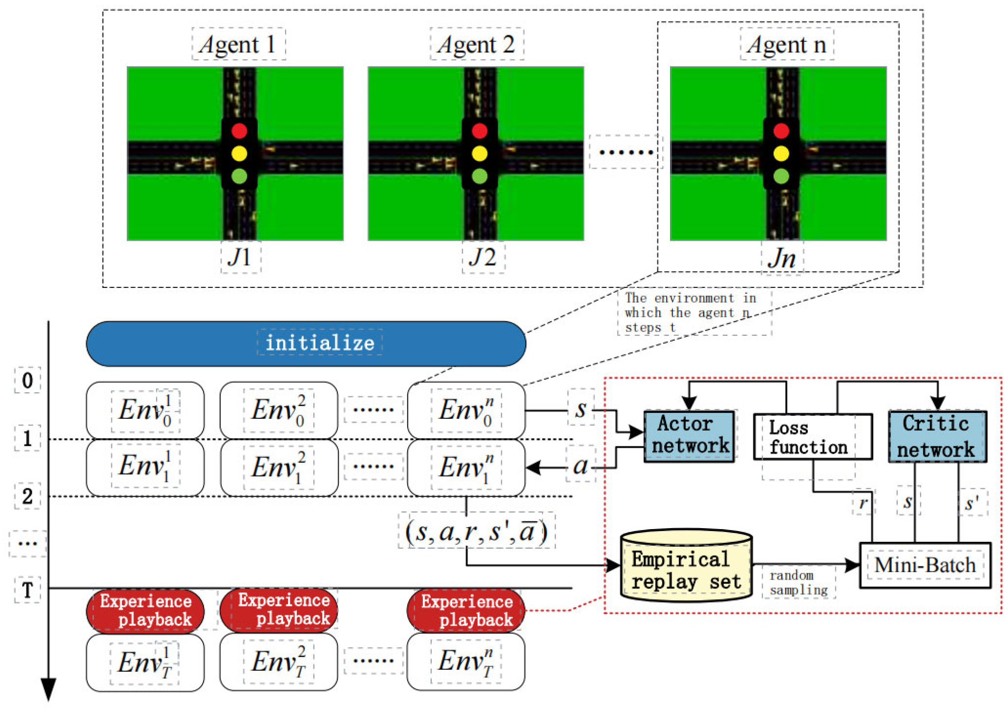
3. Introduction to the MFMARL-ATSC Model Algorithm

In the Mean Field Multi-Agent Reinforcement Learning Area Traffic Signal Control (MFMARL-ATSC) model, the intersection signal control problem is abstracted as a process where agents choose optimal strategies based on regional road network state information. Agents use both dynamic and static traffic information within the road network to select actions from the action space. They record the rewards obtained after executing these actions. Based on the rewards obtained for different actions, agents calculate Q-values, guiding the selection of actions in the next step to achieve the maximum expected outcome.

This model employs a neural network as a function approximator to realize the mean field Q-function in Equation (8), where the Q-function is parameterized by the neural network weights denoted as $\phi$. The update rules in Equation (9) can also be interpreted as adjustments to the neural network weights. As illustrated in Figure 1, the modeling capacity of a convolutional neural network is utilized to compute Q-values for state-action pairs. When fitting Q-values using a convolutional neural network, the state information serves as the input to the network. After processing through the convolutional neural network, the Q-value for the action taken in that state is obtained.

MFMARL-ATSC uses the standard Q-function to solve problems in discrete action space, that is, MFQ-ATSC, shown in Figure 2.where MF is the Mean Field. In the MFQ-ATSC algorithm, the agent is trained by minimizing the loss function:

$$\mathrm{L}\left({\phi }^j\right)={\left(y^j-Q_{{\phi }^j}\left(s,a^j,{\overline{a}}^j\right)\right)}^2$$

where $y^j=r^j+\gamma v_{{\phi }_{\_}^j}^{MF\left(s\prime \right)}$ represents the target mean field value and ${\phi }_{\_}^j$ corresponds to the target network parameters within the neural network. Taking the derivative of the above equation yields the parameter gradient direction as follows:

$${\nabla }_{{\varphi }^j}\mathcal{L}\left({\varphi }^j\right)=\left(y^j-Q_{{\varphi }^j}\left(s,a^j,{\overline{a}}^j\right)\right){\nabla }_{{\varphi }^j}{Q}_{{\varphi }^j}\left(s,a^j,{\overline{a}}^j\right)$$

(13)

The algorithm flow of MFQ-ATSC is as follows (Algorithm 1):

Algorithm 1: MFQ-ATSC

1: Initialize the values of $Q_{{\phi }^j},Q_{{\phi }_{\_}^j}$ and ${\overline{a}}^j$ for all $j\in \left\{\mathrm{1,2},\dots ,N\right\}$.

2: while training is not finished yet do

3:  for $m=1,\dots M$ do

4:   For each intersection agent $j$, sample actions $a^j$ based on the existing average actions ${\overline{a}}^j$ and exploration probabilities, using Equation (13);

5:   For each intersection agent $j$, sample actions ${\overline{a}}^j$ based on Equation (13);

6:  end

7:  Execute the joint action $\mathit{a}=|a^1,\dots ,a^N|$, receive rewards $r=\left[r^1,\dots ,r^N\right]$, and observe the next traffic state s′;

8:  Store $〈s,\mathit{a},\mathit{r},s^{,},\overline{\mathit{a}}〉$ in the replay buffer $\mathcal{D}$, where $\overline{\mathit{a}}=|{\overline{a}}^1,\dots ,{\overline{a}}^N|$;

9:  for $j=1,\dots N$ do

10:   Select a small batch of K experiences $〈s,\mathit{a},\mathit{r},s^{\prime },\overline{\mathit{a}}〉$ from the replay buffer $\mathcal{D}$;

11:   Let ${\overline{a}}_{\_}^j\leftarrow {\overline{a}}^j$, choose actions ${\overline{a}}_{\_}^j$ based on $Q_{{\phi }_{\_}^j}$;

12:   Set $y^j=r^j+\gamma v_{{\phi }_{\_}^j}^{MF}$ according to Equation (11); 13:   Minimize the loss function through $L\left({\phi }^j\right)=\frac{1}{K}\sum {\left(y^j-Q_{{\phi }^j}\left(s^j,a^j,{\overline{a}}^j\right)\right)}^2$; 14:   end 15:  For each intersection agent $j$, the target network parameters are updated based on the learning rate $\tau$: ${\phi }_{\_}^j\leftarrow \tau {\phi }^j+\left(1-\tau \right){\phi }_{\_}^j$; 16: end

Through neural network weights $\theta$, the model’s strategy can be explicitly defined, replacing the Boltzmann strategy used in MFQ-ATSC. This gives rise to the online actor-critic model, shown in Figure 3, namely MFAC-ATSC. The policy network (actor) is trained through the following policy gradient:

$${\nabla }_{{\theta }^j}F\left({\theta }^j\right)\approx {\nabla }_{{\theta }^j}\mathit{log}{\pi }_{{\theta }^j}\left(s\right)Q_{{\varphi }^j}{\left.\left(s,a^j,{\overline{a}}^j\right)\right|}_{a={\pi }_{{\theta }^j}\left(s\right)}$$

In MFAC-ATSC, the critic follows the same configuration as in MFQ-ATSC, as described in Equation (13). During the training process of MFAC-ATSC, it is necessary to continuously update $\theta ,\phi$ until convergence is achieved.

The algorithm flow of MFAC-ATSC is as follows (Algorithm 2):

Algorithm 2: MFAC-ATSC

1: Initialize the values of $Q_{{\phi }^j},Q_{{\phi }_{\_}^j},{\pi }_{{\theta }^j},{\pi }_{{\theta }_{\_}^j}$ and ${\overline{a}}^j$ for all $j\in \left\{\mathrm{1,2},\dots ,N\right\}$.

2: while training is not finished yet do

3:  For each intersection agent, select action $a^j={\pi }_{{\theta }^j}\left(s\right)$ and calculate the new average action $\overline{\mathit{a}}=|{\overline{a}}^1,\dots ,{\overline{a}}^N|$.

4:  Execute the joint action $\mathit{a}=|a^1,\dots ,a^N|$, receive rewards $r=\left[r^1,\dots ,r^N\right]$, and observe the next time step’s traffic state s′

5:  Store $〈s,\mathit{a},\mathit{r},s^{,},\overline{\mathit{a}}〉$ in the replay buffer $\mathcal{D}$;

6:  for $j=1,\dots N$ do

7:   Select a small batch of K experiences $〈s,\mathit{a},\mathit{r},s^{,},\overline{\mathit{a}}〉$ from the replay buffer $\mathcal{D}$;

8:   Set $y^j=r^j+\gamma v_{{\phi }_{\_}^j}^{MF}$ based on Equation (11);

9:   Minimize the loss function through $L\left({\phi }^j\right)=\frac{1}{K}\sum {\left(y^j-Q_{{\phi }^j}\left(s^j,a^j,{\overline{a}}^j\right)\right)}^2$;

10:   Update the actor network with policy gradients as calculated below:       ${\nabla }_{{\theta }^j}F\left({\theta }^j\right)\approx {\nabla }_{{\theta }^j}\mathit{log}{\pi }_{{\theta }^j}\left(s\prime \right)Q_{{\varphi }^j}{\left.\left(s\prime ,a_{\_}^j,{\overline{a}}_{\_}^j\right)\right|}_{a={\pi }_{{\theta }_{\_}^j}\left(s\prime \right)}$

11:  end

12:  Update the target network parameters for each intersection agent $j$ based on the learning rate ${\tau }_{\phi },{\tau }_{\theta }$:          ${\phi }_{\_}^j\leftarrow {\tau }_{\phi }{\phi }^j+\left(1-{\tau }_{\phi }\right){\phi }_{\_}^j$          ${\theta }_{\_}^j\leftarrow {\tau }_{\theta }{\theta }^j+\left(1-{\tau }_{\theta }\right){\theta }_{\_}^j$ 13: end

4. Simulation Experiment Settings and Results Analysis

The experiments in this study were conducted using the open-source simulation software SUMO, which simulates micro-traffic and multi-modal transport. Real-time traffic environment state information was obtained from the Python APIs provided by SUMO, and actions were controlled for traffic signals using the TraCI module.

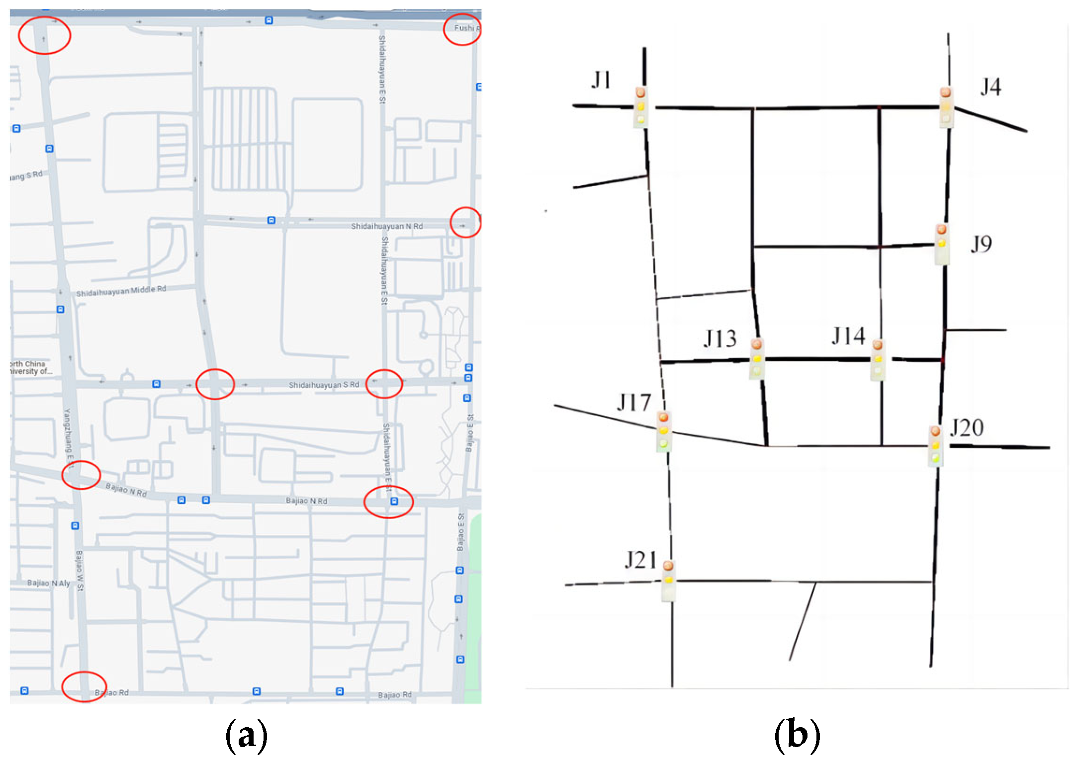
4.1. Simulation Experiment Settings and Results Analysis

The research area selected was the urban road network in Shijingshan District, Beijing. The road network structure in this area is shown in Figure 4a. The area extends north to Fushi Road, east to Bajiao East Street, south to Bajiao Road, and west to Yangzhuang East Street. Within this area, there are various road types, including main roads, secondary roads, and local roads, with lane widths ranging from two lanes in each direction to eight lanes in each direction. There are a total of 22 intersections in the research road network, out of which eight are signal-controlled intersections. In the subsequent research, optimization will be focused exclusively on the signal-controlled intersections marked in Figure 4b.

4.2. Experimental Setup

4.2.1. State Definition

Decisions are made based on the current traffic state, so the design of the state is crucial [16]. The state designed in this study consists of two parts: local information and neighbor information. Local information includes the queue lengths of vehicles in each incoming lane of the current intersection, while neighbor information includes the queue lengths of vehicles in each incoming lane of all neighboring intersections. It is expressed in the following form:

$$s_j=\left[q_j^1,\dots ,q_j^n,q_k^1,\dots ,q_k^n\right]$$

where $q_j^n,q_k^n$ represent the queue length of vehicles in the nth incoming lane for agent $j$ and its neighboring agent $k$.

4.2.2. Action Definition

Agents need to select appropriate actions based on the traffic state and strategy to manage traffic flow. The MFQ-ATSC algorithm uses a standard Q-function to address problems in discrete action spaces, while the MFAC-ATSC algorithm utilizes an AC (Actor-Critic) model to handle continuous action spaces. Consequently, the two algorithms have different action space definitions.

• Discrete Action Space

In the discrete action space, at each step, it is determined whether to increase the current phase’s duration. The action set is as follows:

$$A=\left\{NS{S}_l,NS{S}_s,NS{L}_l,NS{L}_s,WE{S}_l,WE{S}_s,WE{L}_l,WE{L}_s\right\}$$

They represent the following: South–North straight-through phase, lasting 30 s; South–North straight-through phase, lasting 15 s; South–North left-turn phase, lasting 25 s; South–North left-turn phase, lasting 15 s; East–West straight-through phase, lasting 30 s; East–West straight-through phase, lasting 15 s; East–West left-turn phase, lasting 25 s; East–West left-turn phase, lasting 15 s.

2.

Continuous Action Space

In the continuous action space, at each step, it is determined whether to increase the current phase’s duration. The action set is as follows:

$$A=\left\{switch,keep\right\}$$

They represent an immediate switch to the next phase and the maintenance of the current phase, respectively.

4.2.3. Reward Function

Agents adjust the probability distribution of selecting each action based on the received immediate rewards, seeking to maximize long-term reward values [17]. The defined reward in this study is unique for each intersection, meaning that each agent considers only the information within its respective intersection. During the training process, while having knowledge of the states of neighboring intersections and the average actions, agents aim to maximize their accumulated reward. The reward is defined as follows:

$$r=\sum _{n=1}\frac{1}{w_n}$$

where $w_n$ represents the waiting time for the nth incoming lane at the intersection.

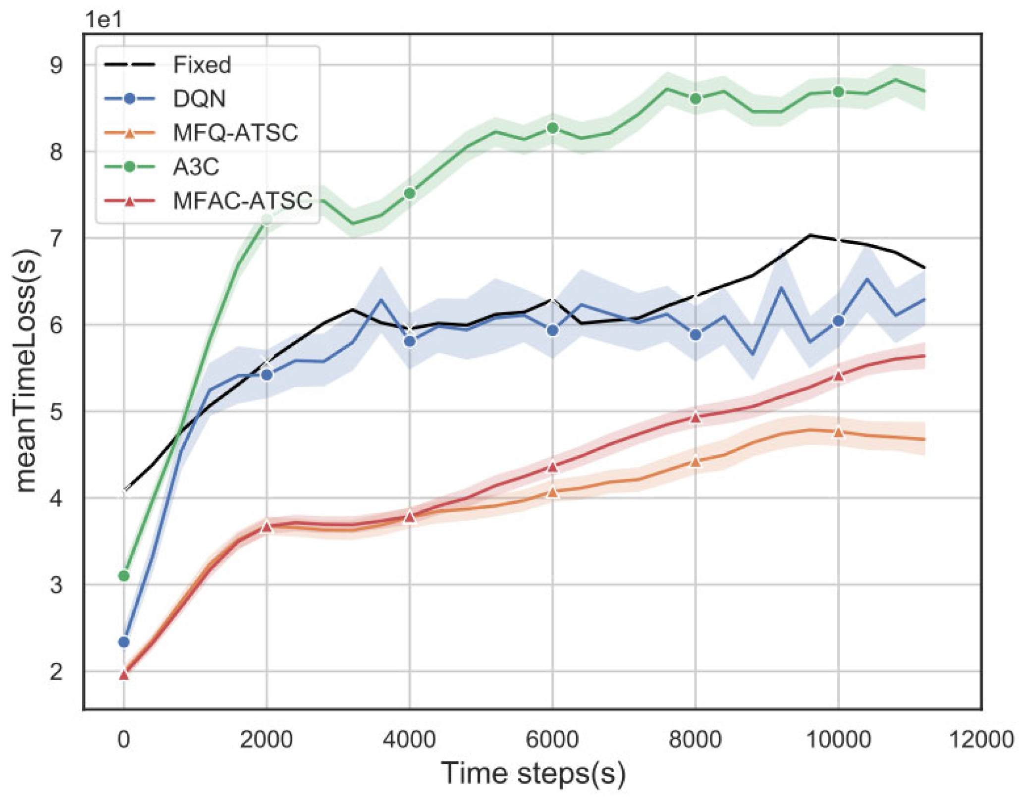
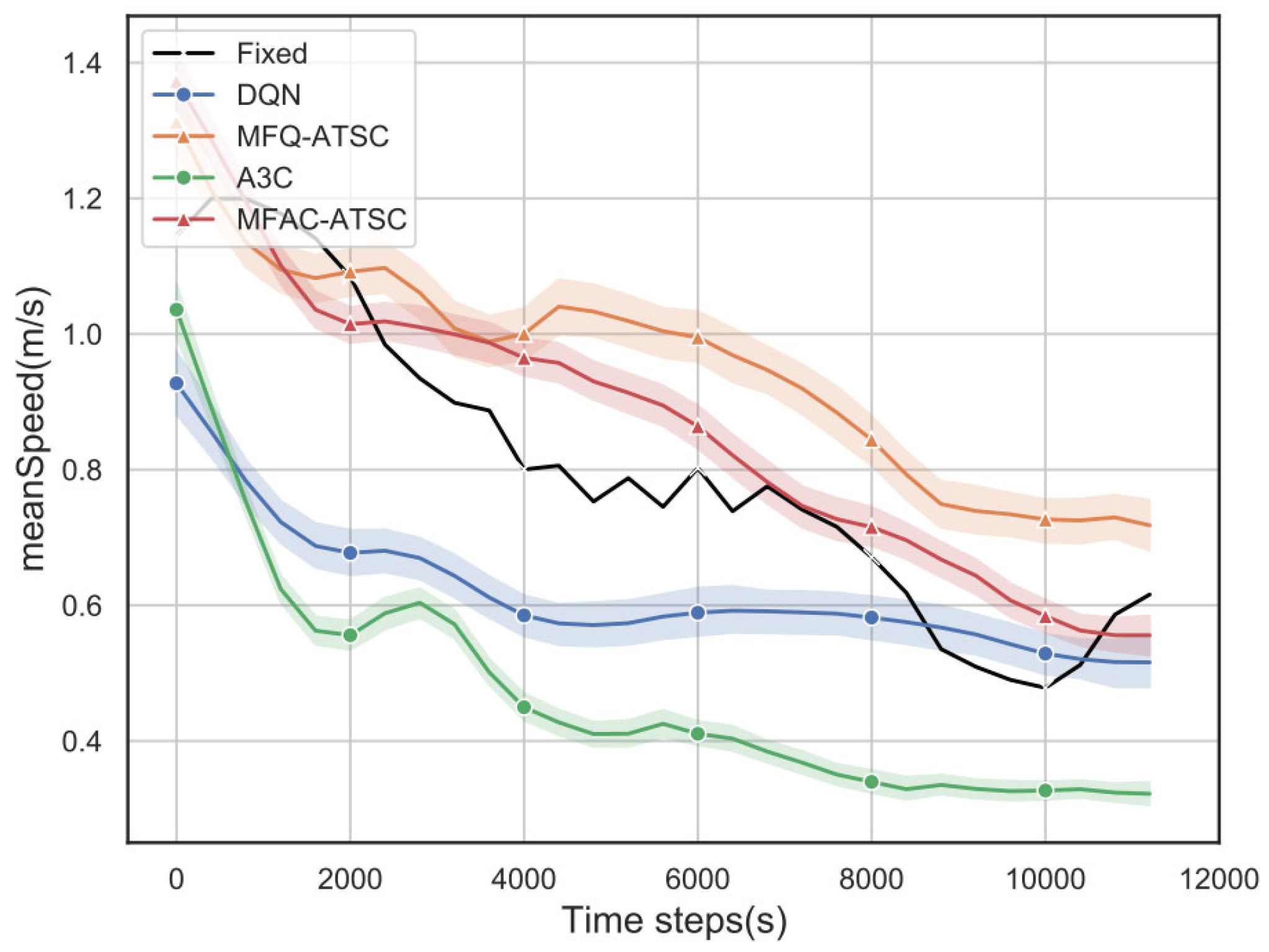
4.3. Simulation Experiment Results Analysis

In this study, a comparison was conducted between the region-based signal traffic control method using MFMARL and traditional signal control methods. The selected control methods included fixed-timing control as well as traditional deep reinforcement learning algorithms like DQN [3] and A3C [18]. DQN and A3C are two algorithms used to solve reinforcement learning problems. They have significant differences in methods and implementation. DQN is a value-based method that aims to directly learn the value function of state-action pairs, often using experience replay and a target network to achieve stable training and convergence. In contrast, A3C combines strategy and value training methods, allowing multiple agents to interact with the environment at the same time, thus improving training efficiency through parallel training and introducing diversity. These were used as control groups in the simulation experiments. When employing the fixed-timing control method, signal timing plans at various intersections within the region remained unchanged and were not adjusted in response to changes in the road network state. In contrast, when employing Mean Field Reinforcement Learning and traditional deep reinforcement learning signal control methods, signal timings at each intersection were dynamically adjusted based on detectors placed within the road network. Each simulation experiment ran for a duration of 10,800 s in each iteration, with a total of 400 iterations. To mitigate potential biases introduced during the road network loading process, no algorithmic control was applied during the initial 1200 s. Figure 5 illustrates the comparison of reward values for various intersections within the region under different control methods.

All the algorithms designed in this study utilize the same neural network structure. As depicted in Figure 5, it is evident that the performance significantly improved when employing the Mean Field Reinforcement Learning control method. Combining the performance of different algorithms across various intersections, it can be observed that the offline learning methods MFQ-ATSC and DQN exhibit faster convergence compared to the online learning methods MFAC-ATSC and A3C [19]. Transforming the multi-intersection traffic signal control problem within the region into interactions between individual intersections and neighboring intersections enhances the convergence speed of offline learning algorithms [20]. During the experience replay process, it allows for faster learning of the optimal policy from non-current strategy experiences [21] and leads to a more stable convergence of the optimal policy [22]. MFQ-ATSC starts converging after 100–150 iterations, while MFAC-ATSC still has a few intersections that have not reached convergence even after 400 iterations.

Based on Figure 4 and Figure 5, and

Table 1. Simulation results at different algorithms.

Evaluation Metrics	Fixed-Timing Control	DQN	MFQ- ATSC	A3C	MFAC- ATSC
Average Reward Value	-	6 × 10−4	1.45 × 10−3	0.7 × 10−4	1.08 × 10−3
Number of Waiting Vehicles	1717	1790	1694	1797	1701
Travel Time (s)	998	993	977	995	986
Loss Time (s)	60.21	56.79	39.44	65.92	42.39
Speed (m/s)	0.81	0.62	0.95	0.57	0.87

, after 400 iterations, it can be observed that the average loss time of MFAC-ATSC is reduced by 29.60% compared with fixed-timing control, while that of MFQ-ATSC is reduced by 34.50%. The huge difference in the J17 reward curve is because J17 is only one agent among multiple agents, and its reward fluctuations cannot fully represent the traffic signal level of the entire area. Judging from the simulation scenario, it is possible that at the intersection where the J17 signal controller is located, vehicle congestion, queuing, sudden braking, and other operations have caused changes in the vehicle density of the road network. The same goes for J9. Furthermore, the control performance is better than the other two traditional deep reinforcement learning control methods. This demonstrates that using mean field reinforcement learning in regional traffic signal control can reduce loss time for vehicles within the road network, thereby improving operational efficiency, as shown in Figure 6 and Figure 7.

5. Conclusions

This article presents a regional traffic signal control method based on mean field reinforcement learning. It trains neural networks based on real-time traffic state information to determine the optimal signal timing plan at intersections. To address the challenges of extending existing multi-agent reinforcement learning algorithms to regional road network environments, such as the problem of dimension explosion and non-stationarity in the environment, mean field multi-agent reinforcement learning decomposes the Q-function through local bilateral interactions. It transforms the multi-agent reinforcement learning problem for regional traffic signal control into an optimization problem of finding the best strategy for the central agent by approximating the mean field. The article applies two mean field multi-agent reinforcement learning algorithms, MFQ-ATSC and MFAC-ATSC, as well as existing DQN and A3C algorithms, to simulate experiments in a real regional road network. These algorithms are compared with traditional fixed-timing control methods. The models are validated using the SUMO simulation platform. MFQ-ATSC and MFAC-ATSC improve travel time by 15.74% and 7.4%, respectively, compared to fixed-timing control. They also outperform the DQN algorithm by 53.22% and 40.32%, respectively, and the A3C algorithm by 85.1% and 52.63%, respectively. The experimental results show that MFQ-ATSC and MFAC-ATSC algorithms converge faster, achieve higher final stable reward values, and result in higher average vehicle speeds and less loss of time within the road network. This demonstrates the effectiveness of mean field multi-agent reinforcement learning algorithms when addressing regional traffic signal control problems, thus significantly improving traffic efficiency within the road network.

Future research will further improve the convergence speed and adaptability of the algorithm and extend the application scope of the model to more complex systems. At the same time, a variety of experimental scenarios will be considered, combined with networked automatic vehicles and regional traffic signal control, and mean field theory will be used to further optimize the traffic efficiency of the road network.

References

1. Hua, W.; Zheng, G.J. Recent Advances in Reinforcement Learning for Traffic Signal Control. ACM SIGKDD Explor. Newsl. 2020, 22, 12–18. [Google Scholar]
2. Mikami, S.; Kakazu, Y. Genetic reinforcement learning for cooperative traffic signal control. In Proceedings of the First IEEE Conference on Evolutionary Computation, IEEE World Congress on Computational Intelligence, Orlando, FL, USA, 27–29 June 1994; Volume 1, pp. 223–228. [Google Scholar]
3. Mnih, V.; Kavukcuoglu, K.; Silver, D.; Rusu, A.A.; Veness, J.; Bellemare, M.G.; Graves, A.; Riedmiller, M.; Fidjeland, A.K.; Ostrovski, G.; et al. Human-level control through deep reinforcement learning. Nature 2015, 518, 529–533. [Google Scholar] [CrossRef] [PubMed]
4. Shang, C.L.; Liu, X.M.; Tian, Y.L.; Tian, Y.L.; Dong, L.X. Priority of Dedicated Bus Arterial Control Based on Deep Reinforcement Learning. J. Transp. Syst. Eng. Inf. Technol. 2021, 21, 64–70. [Google Scholar]
5. Li, L.; Lv, Y.S.; Wang, F.Y. Traffic signal timing via deep reinforcement learning. IEEE/CAA J. Autom. Sin. 2016, 3, 247–254. [Google Scholar]
6. Chu, T.; Wang, J.; Codecà, L.; Li, Z. Multi-Agent Deep Reinforcement Learning for Large-Scale Traffic Signal Control. IEEE Trans. Intell. Transp. Syst. 2020, 21, 1086–1095. [Google Scholar] [CrossRef]
7. Liang, X.; Du, X.; Wang, G.; Han, Z. A Deep Reinforcement Learning Network for Traffic Light Cycle Control. IEEE Trans. Veh. Technol. 2019, 68, 1243–1253. [Google Scholar] [CrossRef]
8. Prashanth, L.A.; Bhatnagar, S. Reinforcement learning with average cost for adaptive control of traffic lights at intersections. In Proceedings of the 2011 14th International IEEE Conference on Intelligent Transportation Systems(ITSC), Washington, DC, USA, 5–7 October 2011; pp. 1640–1645. [Google Scholar]
9. Rasheed, F.; Yau, K.; Low, Y.C. Deep reinforcement learning for traffic signal control under disturbances: A case study on Sunway city, Malaysia. Future Gener. Comput. Syst. 2020, 109, 431–445. [Google Scholar] [CrossRef]
10. Tan, T.; Bao, F.; Deng, Y.; Jin, A.; Dai, Q.; Wang, J. Cooperative Deep Reinforcement Learning for Large-Scale Traffic Grid Signal Control. IEEE Trans. Cybern. 2020, 50, 2687–2700. [Google Scholar] [CrossRef] [PubMed]
11. Zheng, G.; Zang, X.; Xu, N.; Wei, H.; Yu, Z.; Gayah, V.; Xu, K.; Li, Z. Diagnosing Reinforcement Learning for Traffic Signal Control. arXiv 2019, arXiv:abs/1905.04716. [Google Scholar]
12. Xu, M.; Wu, J.; Huang, L.; Zhou, R.; Wang, T.; Hu, D. Network-wide traffic signal control based on the discovery of critical nodes and deep reinforcement learning. J. Intell. Transp. Syst. 2020, 24, 1–10. [Google Scholar] [CrossRef]
13. Yang, Y.; Luo, R.; Li, M.; Zhou, M.; Zhang, W.; Wang, J. Mean Field Multi-Agent Reinforcement Learning. In Proceedings of the 35th International Conference on Machine Learning, Stockholm, Sweden, 10–15 July 2018; Volume 80, pp. 5571–5580. [Google Scholar]
14. Hu, S.; Leung, C.; Leung, H. Modelling the Dynamics of Multiagent Q-Learning in Repeated Symmetric Games: A Mean Field Theoretic Approach. In Proceedings of the Advances in Neural Information Processing Systems 32 (NeurIPS 2019), Vancouver, BC, Canada, 8–14 December 2019. [Google Scholar]
15. Mangasaria, O.L. Equilibrium Points of Bimatrix Games. J. Soc. Ind. Appl. Math. 1964, 12, 778–780. [Google Scholar] [CrossRef]
16. Wu, T.; Zhou, P.; Liu, K.; Yuan, Y.; Wang, X.; Huang, H.; Wu, D.O. Multi-Agent Deep Reinforcement Learning for Urban Traffic Light Control in Vehicular Networks. IEEE Trans. Veh. Technol. 2020, 69, 8243–8256. [Google Scholar] [CrossRef]
17. Kumar, N.; Rahman, S.S.; Dhakad, N. Fuzzy Inference Enabled Deep Reinforcement Learning-Based Traffic Light Control for Intelligent Transportation System. IEEE Trans. Intell. Transp. Syst. 2020, 22, 4919–4928. [Google Scholar] [CrossRef]
18. Mnih, V.; Badia, A.P.; Mirza, M.; Graves, A.; Lilicrap, T.; Herlay, T.; Silver, D.; Kavukcuoglu, K. Asynchronous methods for deep reinforcement learning. In Proceedings of the International Conference on Machine Learning, New York, NY, USA, 19–24 June 2016; pp. 1928–1937. [Google Scholar]
19. Wei, W.; Wu, Q.; Wu, J.Q.; Du, B.; Shen, J.; Li, T. Multi-agent deep reinforcement learning for traffic signal control with Nash Equilibrium. In Proceedings of the 2021 IEEE 23rd International Conference on High Performance Computing & Communications; 7th International Conference on Data Science & Systems; 19th International Conference on Smart City; 7th International Conference on Dependability in Sensor, Cloud & Big Data Systems & Application, Haikou, China, 20–22 December 2021; pp. 1435–1442. [Google Scholar]
20. Zhang, X.; Xiong, G.; Ai, Y.; Liu, K.; Chen, L. Vehicle Dynamic Dispatching using Curriculum-Driven Reinforcement Learning. Mech. Syst. Signal Process. 2023, 204, 110698. [Google Scholar] [CrossRef]
21. Wang, X.; Yang, Z.; Chen, G.; Liu, Y. A Reinforcement Learning Method of Solving Markov Decision Processes: An Adaptive Exploration Model Based on Temporal Difference Error. Electronics 2023, 12, 4176. [Google Scholar] [CrossRef]
22. Wu, Y.; Wu, X.; Qiu, S.; Xiang, W. A Method for High-Value Driving Demonstration Data Generation Based on One-Dimensional Deep Convolutional Generative Adversarial Networks. Electronics 2022, 11, 3553. [Google Scholar] [CrossRef]
Figure 1. Fitting Q-valued convolutional neural networks.
Electronics 12 04686 g001
Figure 2. MFQ-ATSC framework.
Electronics 12 04686 g002
Figure 3. MFAC-ATSC framework.
Electronics 12 04686 g003
Figure 4. Simulation of road network. (a) Target Regional Traffic Network, (b) Simulated Regional Traffic Network.
Electronics 12 04686 g004
Figure 5. The reward value of each intersection is compared under different algorithms.
Electronics 12 04686 g005
Figure 6. Vehicle average loss time using different algorithms.
Electronics 12 04686 g006
Figure 7. Vehicle average speed using different algorithms.
Electronics 12 04686 g007