Abstract
Aiming at the problems of synthetic-aperture radar (SAR), such as high sampling rate and vulnerability to noise interference in imaging, a sparse reconstruction algorithm based on approximate observation and L1/2 threshold iteration is proposed in this paper. To solve the problem of the large dimension and high computational complexity of the measurement matrix, a sparse reconstruction model based on approximate observation is constructed, and a threshold iterative algorithm to rapidly solve the L1/2 regularization problem is introduced, which can realize sparse signal reconstruction with fewer sampling data and quickly solve the problem. The simulation results of point targets and the measured data of spaceborne SAR show that compared with the traditional matched filtering algorithm and L1 threshold algorithm based on a two-step iteration, the proposed sparse reconstruction algorithm has a faster iteration speed and improves the image quality.
1. Introduction
As a microwave remote sensing imaging radar technique, synthetic-aperture radar (SAR) has the characteristics of high azimuth resolution and all-time, all-weather, and long-distance observation ability [1]. However, SAR is susceptible to interference from various factors in practice, which results in missing sampling data and a decreased signal-to-noise ratio (SNR), which lead to degraded imaging quality. Generally, signal sampling must satisfy the Nyquist sampling theorem. The amount of information contained in SAR echo data increases with the amount of echo data obtained via traditional sampling methods, which imposes higher requirements for storage and calculation. Compressive sensing (CS) theory was proposed to cope with this problem, i.e., when the signal is sparse, sparse signal reconstruction can be achieved with less sampling [2]. CS theory has been combined with radar imaging, and theoretical and simulation analyses have verified the feasibility of combining CS theory with SAR imaging [3]. Research has shown that when the imaging scene is sparse, a small number of radar echo data are needed to obtain high-resolution and high-quality SAR images. Sparse SAR imaging technology can effectively reduce the data acquisition and storage requirements of radar receivers. Hence, the correlation imaging method has received extensive attention [4,5,6,7,8].
Traditional sparse SAR imaging requires the construction of an observation matrix, which is closely related to radar system parameters and imaging geometry. The properties of the observation matrix directly affect the signal reconstruction performance. Errors in the observation matrix will lead to phase errors in the SAR data, which can cause the defocusing of the reconstructed image. There are some methods to improve the quality of sparse SAR imaging. A sparse-based SAR joint imaging and phase error correction method has been proposed, which includes image generation and model error correction at each iteration to generate high-quality SAR images [9]. A sparse radar imaging method based on L1/2 regularization theory has been proposed, which uses L1/2 regularization instead of the L1 norm and requires no observation matrix; by constructing a radar echo simulation operator to achieve imaging, the complexity of the algorithm is reduced greatly [10]. A fast compressed sensing SAR imaging method has been proposed that derives an approximate SAR observation model from the inverse of the focusing process, which combines CS and a traditional matched filter into a sparse regularization framework. Then, a fast iterative threshold algorithm is used to solve the sparse image reconstruction problem, which greatly reduces time and storage costs [11]. A sparse autofocus method based on approximate observation and a minimum entropy constraint has been proposed, which introduces a minimum entropy constraint to estimate the error phase and obtains the initial phase via the phase gradient autofocus (PGA) algorithm to reduce the number of iterations [12]. In addition, a sparse SAR autofocus model combining phase error estimation and the L1 norm regularization problem has been proposed. The algorithm can estimate the phase error and obtain high-quality sparse images [13]. A sub-aperture motion state estimation method for airborne SAR platform segment based on parametric sparse representation has been proposed. The SAR echo is expressed as a joint sparse signal by the parametric dictionary matrix, and the SAR motion state estimation is transformed into the dynamic representation of the joint sparse signal, which has a good imaging effect in complex motion environments [14]. An efficient SAR imaging algorithm based on compressed sensing and autofocus fusion has been proposed. The algorithm combines the Tikhonov regularization method and uses an efficient iterative method to effectively solve the optimization problem of spatial phase error variation based on the azimuth domain and low sampling rate [15]. A sparse imaging method based on fusion motion error estimation and compensation has been proposed. This method combines the range-Doppler algorithm with motion error correction to invert the observation model to obtain more accurate estimation results [16].
In the case of SAR with sparse sampling, when the sampling rate of echo data is low, sparse SAR imaging based on L1 regularization has a slow iteration speed and is prone to reconstruction failure [17]. We constructed a new sparse reconstruction model by combining the approximate observation operator [18,19,20] and a new algorithm that can quickly solve the L1/2 regularization problem [21]. The model replaces the observation matrix with an approximate observation operator, which reduces memory usage and accelerates reconstruction. Point target simulation experiments were performed under the conditions of full sampling and undersampling, the results of which show that the proposed sparse reconstruction model shows a certain improvement in image quality compared with the traditional ω-k imaging and L1 threshold iteration algorithms. Moreover, the effectiveness of the proposed sparse reconstruction model was demonstrated by processing spaceborne SAR-measured data.
2. A Sparse Reconstruction Model Based on Approximate Observation
This article mainly studies strip SAR imaging with a side-looking array on airborne or spaceborne data. The range resolution of SAR is achieved by transmitting linear frequency-modulated (LFM) signals, while the azimuth resolution is achieved using the synthetic-aperture principle and coherent-stacking imaging method.
The process of obtaining the scene scattering coefficient using a compressed sensing SAR imaging system can be expressed by a linear time-invariant system, shown as:
where y ∈ CM×1 is the echo data vector, x ∈ CN×1 is the scene scattering coefficient, n ∈ CM×1 is a Gaussian white noise vector, Θ = HΨ ∈ CM×N is the observation matrix, H ∈ CM×M is the sparse microwave imaging undersampling matrix, and Ψ ∈ CM×N is the measurement matrix. M is the number of sampling points of echo data, which is determined using the radar resolution theory and Nyquist sampling theorem. N is the number of sampling points in the scene, which is determined by the size of the observation scene.
Formula (1) can be solved via L1 norm regularization, expressed as:
where λ > 0 is the regularization parameter, and ‖·‖2 and ‖·‖1 represent the L2 norm and L1 norm, respectively.
When the SAR echo data have a phase error, Formula (2) is rewritten as [9]:
where Φ is the phase error matrix, i.e.:
When using a sparse reconstruction algorithm for SAR imaging, it is necessary to change the echo data from a two-dimensional matrix to a one-dimensional vector. If the echo data have more sampling values, or the spatial scale of the imaging scene is large, the data consume a large amount of memory, and imaging requires much time. Hence, imaging based on sparse reconstruction has high computational complexity and poor real-time performance, which is not suitable for the real-time imaging of large scenes. Given the above problems, a sparse imaging method based on approximate observation is proposed. The approximate observation operator was used instead of matrix multiplication to construct a new sparse autofocus model, which greatly reduced the dimensions of the observation matrix and improved the reconstruction efficiency and imaging quality.
In this paper, we took the wavenumber domain (ω-k) imaging algorithm as an example to construct the approximate observation operator [22]. This algorithm uses the reference function of the azimuth–range two-dimensional frequency domain to realize two-dimensional pulse compression and uniform range migration correction, and uses Stolt interpolation to realize the focusing of other targets.
The imaging operator based on the ω-k algorithm is expressed as:
where Y represents the original echo data of two-dimensional SAR, Fa and Fr are the respective azimuth and range Fourier transforms, Fa−1 and Fr−1 are the respective azimuth and range Fourier inverse transforms, θref is the uniform range migration correction matrix, and S(·) is the Stolt interpolation operator.
The expression of θref is:
where ft and fτ are the respective azimuth and range frequency, Rref is the reference slant range, fc is the signal carrier frequency, vrc is the radar effective speed, Kr is the range modulation frequency, and c is the speed of light.
The expression of S(·) is [23]:
The approximate observation operator is obtained by inverting the imaging operator, shown as:
where X is the two-dimensional focused SAR image of the observed scene, S−1(·) is the inverse mapping of S(·), and (·)* is the conjugate of a matrix.
By introducing the approximate observation operator into formula (3), a sparse autofocus model based on approximate observation can be obtained as:
where L is the undersampling matrix of the echo.
To introduce the traditional matched filtering algorithm into the above model, the imaging operator Iω-k(·) is decomposed into the phase correction operator Ω(·) and azimuth Fourier transform operator Fa(·), which are expressed as [12]:
The Γ(·) is the imaging operator, which can be expressed as:
and we rewrite Formula (9) as:
where Ω−1(·) denotes the inverse-phase correction operator.
3. Iterative Thresholding Algorithm
3.1. L1/2 Threshold Iterative Algorithm
Formula (13) is an L1 regularization problem, which can be solved via gradient descent, iterative soft thresholding, and other methods. With the development of compressed sensing, it is found that L1 regularization based on convex relaxation does not produce enough sparse solutions. When q ∈ (0,1/2), the regularization performance is not significantly improved; when q ∈ (1/2,1), the regularization performance gradually decreases, and the sparsest result can be achieved when q = 1/2. Therefore, the L1/2 regularization is introduced, which can realize sparse signal reconstruction with less sampling and obtain a quick solution [24,25,26].
The L1/2 threshold iterative algorithm is expressed as:
where μ is the iteration step size, which is related to whether the iterative process converges; (·)H represents the conjugate transpose of a matrix; and Hλ,μ,1/2 represents the threshold operator expressed by:
where (·)T represents the transpose of a matrix, and ηλ,μ,1/2 denotes the threshold function:
where:
3.2. Fast Threshold Iterative Algorithm for the L1/2 Regularization Problem
The accelerated proximal gradient algorithm is used to solve the L1/2 regularization problem [21], which has the following iterative steps.
Step 1: Given an initial value x0 = x1= 0, let t0 = 1 and k = 0, and set the threshold to ε.
Step 2: Calculate:
where L is the Lipschitz constant of the derivative of f(x).
Step 3: The iteration stops when ‖xk+1-xk‖2/‖xk‖2 < ε.
Here, the threshold ε is a very small value (such as 10−6). In different applications of the algorithm, ε can be determined through experimental methods.
4. Sparse Reconstruction Algorithm Based on Approximate Observation and L1/2 Threshold Iteration
We constructed a new sparse reconstruction model by combining the threshold iteration algorithm, which can quickly solve the L1/2 regularization problem, with the approximate observation operator based on the ω-k algorithm. The model is solved via a two-step iteration, including the reconstruction of x and Φ. The pseudocode of the solution process is given as follows Algorithm 1.
| Algorithm 1 Sparse Reconstruction Algorithm Based on Approximate Observation and L1/2 Threshold Iteration |
| Initialization: i = 0, Imax is the maximum number of iterations, R0 = 0, t0 = 1, Φ0 = PGA(Γ(L⊙y)). |
| Iterative process: for i = 1: Imax. |
| The algorithm stops when ‖xi+1-xi‖2/‖xi‖2 < ε. |
In Algorithm 1, the appropriate Φ0 can reduce the number of iterations, so the phase gradient autofocus (PGA) algorithm [27] is used to provide Φ0. μ usually takes a value of 1 to ensure convergence. The parameter λ is related to the sparsity K of the imaging scene, which is expressed as:
where |Ri|K+1 is the amplitude value of (K + 1) in the order of magnitude of all elements in the matrix Ri.
Therefore, after obtaining the sparsely sampled data and the imaging operator based on the matched filtering algorithm, sparse SAR imaging can be realized using the above algorithm.
5. Experiments and Result Analysis
The point target simulation and SAR-measured data of a simulated scene were used to verify the effectiveness of the proposed sparse reconstruction algorithm. Compared with the traditional ω-k imaging algorithm and the L1 threshold algorithm based on a two-step iteration, the advantages of the proposed algorithm in imaging quality and convergence speed were analyzed.
5.1. Point Target Simulation Data Experiment under Full Sampling
Three-point-target simulation data in the simulation scene were used for experimental verification. The point targets were sparse in the simulation scene. The parameters of the simulation experiment are shown in Table 1.

Table 1.
SAR imaging simulation parameters.
Three-point targets were set in the simulated scene. In order to facilitate an intuitive comparison of the convergence speed and accuracy of the algorithm, the number of iterations in the algorithm and the comparison algorithm was fixed at 5. The above four imaging algorithms were used for imaging, respectively, and the results are shown in Figure 1. Figure 1a shows the imaging result of the traditional ω-k imaging algorithm. It can be seen that the three-point targets had high side lobes. Figure 1b shows the imaging results of the iterative shrinkage thresholding algorithm. The side lobe of the point target was reduced and the image quality was enhanced. Figure 1c shows the imaging result of the L1 threshold algorithm based on a two-step iteration, where the side lobe of the point target was significantly reduced, and the imaging quality was improved. Figure 1d shows the imaging result of the proposed sparse reconstruction algorithm; compared with the other algorithms, the energy of the target was significantly improved, as was the imaging quality.
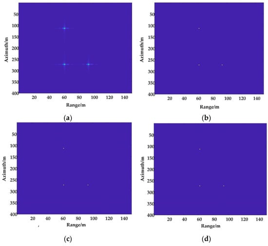
Figure 1.
Point target simulation results. (a) traditional ω-k imaging algorithm; (b) iterative shrinkage thresholding algorithm; (c) L1 threshold algorithm based on the proposed two-step iteration; (d) proposed sparse reconstruction algorithm.
Figure 2 shows the cross-section of the imaging results of the above four methods in the azimuth direction. It can be seen that the traditional ω-k imaging algorithm had the worst resolution in the azimuth direction. Compared with the traditional algorithm, the resolution in the azimuth direction of the L1 threshold algorithm based on a two-step iteration and the iterative shrinkage thresholding algorithm was greatly improved. The resolution of the proposed sparse reconstruction algorithm was slightly better than that of the L1 threshold algorithm based on a two-step iteration.
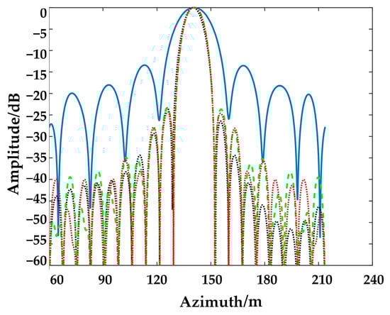
Figure 2.
Point target profile. —, traditional ω-k imaging algorithm; ---, L1 threshold algorithm based on the proposed two-step iteration; …., proposed sparse reconstruction algorithm; …., iterative shrinkage thresholding algorithm.
To further verify the improvement in the imaging quality by the proposed sparse reconstruction algorithm, the peak side lobe ratio (PSLR), integral side lobe ratio (ISLR), and impulse response width (IRW) of the point targets were quantitatively analyzed, with the results shown in Table 2. It can be seen that, compared with the other three algorithms, the azimuth resolution of the proposed sparse reconstruction algorithm was the highest, and its PSLR was the lowest. Hence, the weak target in the main lobe was not easily submerged by the adjacent strong target in the side lobe. Through the numerical comparison of relevant parameters, the advantages of the proposed sparse reconstruction algorithm were verified.
Table 2.
Point target center azimuth indicator.
Table 3 shows the operation time of the sparse reconstruction algorithm and the L1 threshold algorithm based on a two-step iteration. In the same computer configuration (CPU: AMD Ryzen 5 5600H with Radeon Graphics(Advanced Micro Devices, San Jose, CA, USA); main frequency: 3.30 GHz; memory: 16.0 GB), the operation time of each algorithm was recorded through simulation experiments. It shows that the proposed sparse reconstruction algorithm has a higher convergence rate than the L1 threshold algorithm. Hence, the proposed algorithm has a great advantage in real-time imaging for SAR.
Table 3.
Calculation of time consumption.
5.2. Simulation Results of Random Missing Data in the Azimuth Direction
We analyzed the image quality when random missing data appeared in the azimuth direction. The initial data were the data of azimuth full aperture, which satisfies the Nyquist sampling law. The four algorithms use point targets with random losses of 30% and 70% data in the azimuth direction for imaging. Figure 3a and Figure 4a show the respective imaging results of the traditional ω-k imaging algorithm with 30% and 70% of the data missing randomly in the azimuth direction. Figure 3b and Figure 4b show the respective imaging results of the iterative shrinkage thresholding algorithm with 30% and 70% of the data missing randomly in the azimuth direction. Figure 3c and Figure 4c show the respective imaging results of the L1 threshold algorithm based on a two-step iteration under the condition of randomly missing 30% and 70% of data in the azimuth direction. Figure 3d and Figure 4d show the respective imaging results of the proposed algorithm under the random loss of 30% and 70% of data in the azimuth direction. It can be seen that, compared with the traditional ω-k imaging algorithm, the imaging results of the other three algorithms were clearer, the image quality was higher, and the focusing performance was significantly improved.
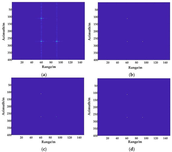
Figure 3.
Simulation results of point targets with 30% missing azimuth data. (a) ω-k imaging algorithm when 30% of azimuth data are missing; (b) iterative shrinkage thresholding algorithm when 30% of azimuth data are missing; (c) L1 threshold algorithm based on the proposed two-step iteration when 30% of azimuth data are missing; (d) sparse reconstruction algorithm when 30% of azimuth data are missing.
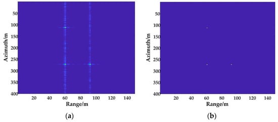
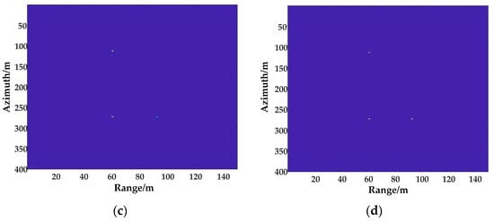
Figure 4.
Simulation results of point targets with 70% missing azimuth data. (a) ω-k imaging algorithm when 70% of azimuth data are missing; (b) iterative shrinkage thresholding algorithm when 70% of azimuth data are missing; (c) L1 threshold algorithm based on the proposed two-step iteration when 70% of azimuth data are missing; (d) sparse reconstruction algorithm when 70% of azimuth data are missing.
Figure 5 and Figure 6 show the point target profiles with 30% and 70% randomly missing echo data, respectively. From the image results, the performance of the proposed algorithm was the best in all aspects. Therefore, it has advantages in improving image quality.
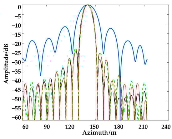
Figure 5.
Point target profile with 30% missing azimuth data. —, traditional ω-k imaging algorithm; ---, L1 threshold algorithm based on the proposed two-step iteration; …., proposed sparse reconstruction algorithm; …., iterative shrinkage thresholding algorithm.
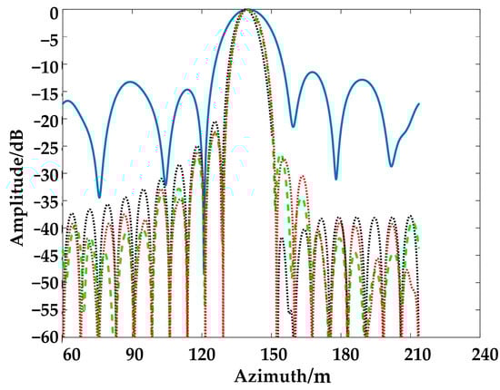
Figure 6.
Point target profile with 70% missing azimuth data. —, traditional ω-k imaging algorithm; ---, L1 threshold algorithm based on the proposed two-step iteration; …., proposed sparse reconstruction algorithm; …., iterative shrinkage thresholding algorithm.
Table 4 and Table 5 show the quantitative analysis of PSLR, ISLR, and IRW of a point target under the conditions of 30% and 70% randomly missing echo data. Based on these results, the proposed algorithm was superior in all aspects, and hence, it has advantages in image quality improvement.
Table 4.
Target center azimuth performance with 30% missing azimuth data.
Table 5.
Target center azimuth performance with 70% missing azimuth data.
5.3. Simulation Analysis of the Imaging Results after Adding Noise
Gaussian white noise was added to the echo data of point targets in a simulated scene. With SNRs of 10 dB and −10 dB, the traditional ω-k imaging algorithm, iterative shrinkage thresholding algorithm, L1 threshold algorithm based on a two-step iteration, and proposed algorithm were used for imaging. By comparing their results, the denoising effect of the proposed sparse reconstruction algorithm was verified.
Figure 7a and Figure 8a show the imaging results of the traditional ω-k imaging algorithm with SNRs of 10 dB and −10 dB, respectively. The imaging results of the traditional ω-k imaging algorithm had significant background noise, and the imaging quality was greatly reduced. Figure 7b and Figure 8b show the imaging results of the iterative shrinkage thresholding algorithm with SNRs of 10 dB and −10 dB, respectively. The results show that under different signal-to-noise ratios, the target was clearer, all the background noise was filtered out, and the side lobe was also well suppressed. Figure 7c and Figure 8c show the imaging results of the L1 threshold algorithm based on a two-step iteration with SNRs of 10 dB and −10 dB, respectively. The results have clear point targets under different SNRs, almost all background noises were filtered out, and the side lobes were better suppressed. Figure 7d and Figure 8d show the imaging results of the proposed sparse reconstruction algorithm under SNRs of 10 dB and −10 dB, respectively. It can be seen that it demonstrated the high definition of target points and a good suppression of side lobes with an SNR of −10 dB, and, hence, has superior image-focusing performance under low SNRs.
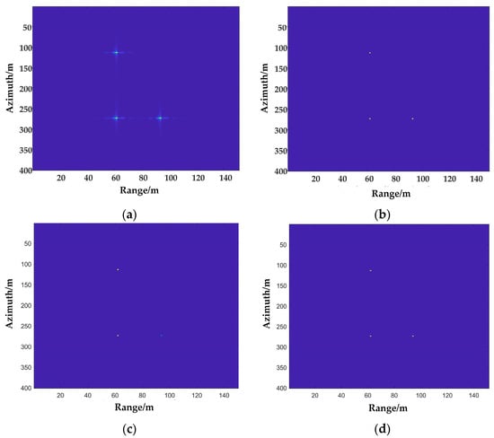
Figure 7.
Simulation results of point targets with an SNR of 10 dB. (a) traditional ω-k imaging algorithm (SNR = 10 dB); (b) iterative shrinkage thresholding algorithm (SNR = 10 dB); (c) L1 threshold algorithm based on the proposed two-step iteration (SNR = 10 dB); (d) proposed sparse reconstruction algorithm (SNR = 10 dB).
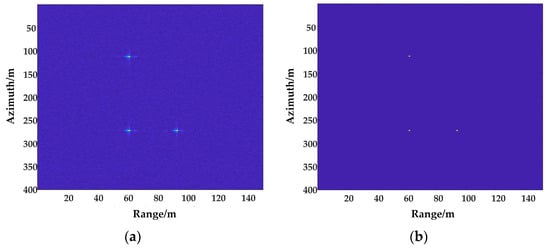
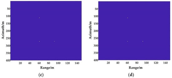
Figure 8.
Simulation results of point targets with an SNR of −10 dB. (a) traditional ω-k imaging algorithm (SNR = −10 dB); (b) iterative shrinkage thresholding algorithm (SNR = −10 dB); (c) L1 threshold algorithm based on the proposed two-step iteration (SNR = −10 dB); (d) proposed sparse reconstruction algorithm (SNR = −10 dB).
Figure 9 and Figure 10 depict the point target profiles with signal-to-noise ratios of 10 dB and −10 dB, respectively. From the images, it can be seen that the proposed algorithm has advantages in improving image quality compared with the other methods.
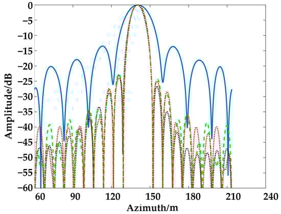
Figure 9.
Point target profile with an SNR of 10 dB. —, traditional ω-k imaging algorithm; ---, L1 threshold algorithm based on the proposed two-step iteration; …., proposed sparse reconstruction algorithm; …., iterative shrinkage thresholding algorithm.
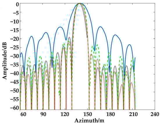
Figure 10.
Point target profile with an SNR of −10 dB. —, traditional ω-k imaging algorithm; ---, L1 threshold algorithm based on the proposed two-step iteration; …., proposed sparse reconstruction algorithm; …., iterative shrinkage thresholding algorithm.
Table 6 and Table 7 describe point targets with signal-to-noise ratios of 10 dB and −10 dB. Based on these results, the proposed algorithm is optimal in all aspects. Hence, it has advantages in image quality improvement.
Table 6.
The azimuth performance of the target center with an SNR of 10 dB.
Table 7.
The azimuth performance of the target center with an SNR of −10 dB.
5.4. Analysis of the Imaging Results with Measured Data
The effectiveness of the proposed sparse reconstruction algorithm was verified with SAR-measured data. The data from the RADARSAT-1 radar satellite launched by the Canadian Space Agency were selected for the experiment, with parameters set as shown in Table 8. The following images are the imaging results under the condition of the random loss of 30% data in the azimuth direction. Figure 11a shows the imaging results of the traditional ω-k imaging algorithm. Figure 11b shows the results of the iterative shrinkage thresholding algorithm. Figure 11c shows the results of the L1 threshold algorithm based on a two-step iteration. Figure 11d shows the imaging results of the proposed sparse reconstruction algorithm. It can be seen from the results that all four algorithms can accurately focus on the positions of the targets. However, there is more noise in Figure 11a, the ship images are not clear, and there are obvious side lobes. In Figure 11b, part of the noise is filtered out, the target point of the ship is clear, and some side lobes are suppressed. In Figure 11c, the noise is filtered out, the strong target points of the ship are clear, and the side lobe is well suppressed. It can be seen from Figure 11d that the proposed algorithm can eliminate the imaging side lobe of the ship targets. The imaging effect of the weak target is better than that of the two-step iterative L1 threshold algorithm, the noise is effectively eliminated, and the imaging quality is improved.
Table 8.
RADARSAT-1 satellite SAR imaging parameters.
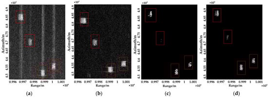
Figure 11.
Imaging results of SAR-measured data. (a) traditional ω-k imaging algorithm; (b) iterative shrinkage thresholding algorithm; (c) L1 threshold algorithm based on the proposed two-step iteration; (d) proposed sparse reconstruction algorithm.
5.5. Limitations of the Method
The limitations of the sparse reconstruction algorithm were demonstrated by the SAR-measured data. Figure 12a shows the imaging results of ω-k in a nonsparse scene; Figure 12b shows the imaging results of the proposed algorithm for the same scenes. It can be seen from the imaging results that, in nonsparse scenes, the imaging quality of the proposed algorithm is even worse than the traditional algorithms. Hence, the proposed algorithm based on sparse reconstruction is more suitable for sparse scenes; otherwise, the imaging quality is degraded.
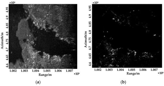
Figure 12.
Imaging results of SAR-measured data in nonsparse scenes. (a) Traditional ω-k imaging algorithm; (b) proposed sparse reconstruction algorithm.
6. Conclusions
In this paper, a sparse reconstruction model based on approximate observation, a two-step iterative sparse reconstruction algorithm, and an L1/2 iterative threshold algorithm were studied for the first time. Based on these, a sparse imaging algorithm based on L1/2 threshold iteration and an approximate observation operator was proposed. This algorithm iteratively solves the scene scattering coefficient and phase error as independent variables and uses the L1/2 norm to improve the sparsity of the reconstruction results and the self-focusing effect of the target. The experimental imaging results of the simulated and measured data showed that the proposed algorithm has a good imaging effect on the target in the case of more random missing data in the azimuth direction. Compared with the iterative shrinkage thresholding algorithm and the L1 threshold algorithm based on a two-step iteration, the efficiency of the proposed algorithm was significantly improved, and the real-time imaging performance was enhanced. In addition, in the case of low SNRs of SAR sampling data, the proposed algorithm could filter out the noise well and ensure a strong imaging effect of the target. Moreover, the proposed algorithm is more suitable for sparse scenes. In nonsparse scenes, the imaging quality was even worse than that of traditional algorithms. In the future, we will study the autofocus method in nonsparse scenarios.
Author Contributions
Conceptualization, Z.G. and X.L.; methodology, X.L.; software, Z.G. and X.L.; validation, Z.G. and X.L.; formal analysis, Z.G.; investigation, Z.G., X.L., and P.H.; resources, Z.G. and X.L.; data curation, Z.G. and X.L.; writing—original draft preparation, X.L.; writing—review and editing, Z.G. and P.H.; visualization, X.L.; supervision, W.X. and W.T.; project administration, Z.G. and P.H.; funding acquisition, Z.G. and P.H. All authors have read and agreed to the published version of the manuscript.
Funding
This work was supported in part by the National Natural Science Foundation of China under grant no. 61761037, the Natural Science Foundation of Inner Mongolia under grant no. 2021MS06005, and the Basic Scientific Research Business Cost Project of Colleges of Inner Mongolia under grant no. JY20220147.
Data Availability Statement
Data are contained within the article.
Conflicts of Interest
The authors declare no conflict of interest.
References
- Moreira, A.; Prats-Iraola, P.; Younis, M.; Krieger, G.; Hajnsek, I.; Papathanassiou, K.P. A tutorial on synthetic aperture radar. IEEE Geosci. Remote Sens. Mag. 2013, 1, 6–43. [Google Scholar] [CrossRef]
- Donoho, D.L. Compressed sensing. IEEE Trans. Inf. Theory 2006, 52, 1289–1306. [Google Scholar] [CrossRef]
- Baraniuk, R.; Steeghs, P. Compressive Radar Imaging. In Proceedings of the 2007 IEEE Radar Conference, Waltham, MA, USA, 17–20 April 2007. [Google Scholar]
- Li, G.; Ma, Y.; Dong, J. Total variation regularization-based compressed sensing synthetic aperture radar imaging. J. Appl. Remote Sens. 2018, 12, 045017. [Google Scholar] [CrossRef]
- Ni, J.C.; Zhang, Q.; Luo, Y.; Sun, L. Compressed sensing SAR imaging based on centralized sparse representation. IEEE Sens. J. 2018, 18, 4920–4932. [Google Scholar] [CrossRef]
- Bi, H.; Zhang, B.C.; Hong, W.; Wu, Y.R. Validation of sparse SAR imaging method based on complex image on GF-3 data. J. Radar 2020, 9, 123–130. [Google Scholar]
- Yang, L.; Li, P.C.; Li, H.J.; Fang, C. Robust and efficient general SAR image sparse feature enhancement algorithm. J. Electron. Inform. 2019, 41, 2826–2835. [Google Scholar]
- Wang, T.Y.; Liu, B.; Wei, Q.; Kang, K.; Yu, Q.H.; Cong, B. Research progress of compressed sensing imaging radar. Electro Opt. Control. 2019, 26, 1–8. [Google Scholar]
- Onhon, N.Ö.; Cetin, M. A sparsity-driven approach for joint SAR imaging and phase error correction. IEEE Trans. Image Process. 2012, 21, 1306–1319. [Google Scholar] [CrossRef] [PubMed]
- Xu, Z.B.; Wu, Y.R.; Zhang, B.C.; Wang, Y. Sparse radar imaging based on L1/2 regularization theory. Sci. Instrum. News 2018, 63, 6–43. [Google Scholar]
- Fang, J.; Xu, Z.; Zhang, B.; Hong, W.; Wu, Y. Fast compressed sensing SAR imaging based on approximated observation. IEEE J. Sel. Top. Appl. Earth Obs. Remote Sens. 2014, 7, 352–363. [Google Scholar] [CrossRef]
- Xiong, X.Y.; Li, G.; Ma, Y.H. SAR sparse autofocusing method based on approximate observation and minimum entropy constraint. Syst. Eng. Electron. 2021, 43, 2803–2811. [Google Scholar]
- Zhang, J.J.; Lu, X.M.; Bi, H.; Song, Y.F.; Yu, D.S. Sparse stripmap SAR autofocusing imaging combining phase error estimation and L₁-norm regularization reconstruction. IEEE Trans. Geosci. Remote Sens. 2023, 61, 1–12. [Google Scholar] [CrossRef]
- Chen, Y.C.; Li, G.; Zhang, Q.; Zhang, Q.J.; Xia, X.G. Motion compensation for airborne SAR via parametric sparse representation. IEEE Trans. Geosci. Remote Sens. 2017, 55, 551–562. [Google Scholar] [CrossRef]
- Kang, M.S.; Baek, J.M. Efficient SAR imaging integrated with autofocus via compressive sensing. IEEE Geosci. Remote Sens. Lett. 2022, 19, 3213251. [Google Scholar] [CrossRef]
- Pu, W.; Wu, J.J.; Wang, X.D.; Huang, Y.; Zha, Y.; Yang, J. Joint sparsity-based imaging and motion error estimation for BFSAR. IEEE Trans. Geosci. Remote Sens. 2019, 57, 1393–1408. [Google Scholar] [CrossRef]
- Bi, H.; Bi, G. Performance Analysis of Iterative Soft Thresholding Algorithm for L1 Regularization Based Sparse SAR Imaging. In Proceedings of the 2019 IEEE Radar Conference, Boston, MA, USA, 22–26 April 2019. [Google Scholar]
- Bi, H.; Zhu, D.; Bi, G.; Zhang, B.; Hong, W.; Wu, Y. FMCW SAR sparse imaging based on approximated observation: An overview on current technologies. IEEE J. Sel. Top. Appl. Earth Obs. Remote Sens. 2020, 13, 4825–4835. [Google Scholar] [CrossRef]
- Wang, Z.; Liu, F.; Yin, Y.; Li, B.; Guo, Y. Weighted L1-Norm for One-Bit Compressed Sensing Based on Approximated Observation. In Proceedings of the 2020 IEEE MTT-S International Wireless Symposium (IWS), Shanghai, China, 20–23 September 2020. [Google Scholar]
- Li, B.; Liu, F.; Zhou, C.; Wang, Z.; Han, H. Mixed sparse representation for approximated observation-based compressed sensing radar imaging. J. Appl. Remote Sens. 2018, 12, 035015. [Google Scholar] [CrossRef]
- Xie, L.L. A New Algorithm for Fast Solving L1/2 Regularization Problem. Master’s Thesis, DaLian University of Technology, DaLian, China, 2014. [Google Scholar]
- Sahay, P.; Vaidya Dhavalkumar, B.; Lokesh Kiran, K. Squint SAR Algorithm for Real-Time SAR Imaging. In Proceedings of the 2022 IEEE International Conference on Electronics, Computing and Communication Technologies (CONECCT), Bangalore, India, 8–10 July 2022. [Google Scholar]
- Wu, Y.Y.; Hong, W.; Zhang, B.C. Introduction to Sparse Microwave Imaging, 3rd ed.; Science Press: Beijing, China, 2021; pp. 99–101. [Google Scholar]
- Xu, Z.B. Data Modeling: Visual Psychology Approach and L1/2 Regularization Theory. In Proceedings of the International Congress of Mathematicians 2010, ICM 2010, Hyderabad, India, 19–27 August 2010. [Google Scholar]
- Zeng, J.; Lin, S.; Wang, Y.; Xu, Z. L1/2 regularization: Convergence of iterative half thresholding algorithm. IEEE Trans. Signal Process. 2014, 62, 2317–2329. [Google Scholar] [CrossRef]
- Xu, Z.; Chang, X.; Xu, F.; Zhang, H. L1/2 regularization: A thresholding representation theory and a fast solver. IEEE Trans. Neural Netw. Learn. Syst. 2012, 23, 1013–1027. [Google Scholar] [PubMed]
- Wahl, D.E.; Eichel, P.H.; Ghiglia, D.C.; Jakowatz, C.V. Phase gradient autofocus—A robust tool for high resolution SAR phase correction. IEEE Trans. Aerosp. Electron. Syst. 1994, 30, 827–835. [Google Scholar] [CrossRef]
Disclaimer/Publisher’s Note: The statements, opinions and data contained in all publications are solely those of the individual author(s) and contributor(s) and not of MDPI and/or the editor(s). MDPI and/or the editor(s) disclaim responsibility for any injury to people or property resulting from any ideas, methods, instructions or products referred to in the content. |
© 2023 by the authors. Licensee MDPI, Basel, Switzerland. This article is an open access article distributed under the terms and conditions of the Creative Commons Attribution (CC BY) license (https://creativecommons.org/licenses/by/4.0/).