Fast Health State Estimation of Lead–Acid Batteries Based on Multi-Time Constant Current Charging Curve

Abstract

Lead–acid batteries are widely used, and their health status estimation is very important. To address the issues of low fitting accuracy and inaccurate prediction of traditional lead–acid battery health estimation, a battery health estimation model is proposed that relies on charging curve analysis using historical degradation data. This model does not require the assistance of battery mechanism models or empirical degradation models, instead, it is combined with improved deep learning algorithms. A long short-term memory (LSTM) regression model was established, and parameter optimization was performed using the bat algorithm (BA). The experimental results show that the proposed model can achieve an accurate capacity estimation of lead–acid batteries.

1. Introduction

The battery is a vital energy storage device widely utilized in various sectors, including automobiles, power, and communication. However, issues such as aging of electrode plates, sulfation, and grid corrosion drastically reduce the battery’s capacity, leading to premature failure. Accurate prediction of state of health (SOH) can provide a reliable basis for battery replacement and reduce the cost of battery pack replacement. At present, the mainstream power batteries on the market are categorized as lead–acid batteries and lithium batteries. When compared to the extensive research conducted on SOH estimation of lithium batteries, the research conducted on lead–acid batteries is significantly less. Therefore, we will also refer to the latest literature on lithium-ion batteries, which can aid us in better assessing the advantages and disadvantages of the SOH estimation methods.

Capacity degradation is the main failure mode of lead–acid batteries. Therefore, it is equivalent to predict the battery life and the change in battery residual capacity in the cycle. The definition of SOH is shown in Equation (1):

$$SoH=\frac{C_t}{C_0}$$

(1)

where C_t is the actual capacity, C₀ is nominal capacity. In other words, SOH is the ratio of the actual capacity and nominal capacity of a battery [1]; when the SOH of the battery reaches 80%, the battery reach its end of life [2].

Shida Jiang et al. divided SOH estimation methods into four categories: direct measurement-based methods, model-based methods, data-driven methods, and hybrid methods [3]. Lei Zhen et al. combined the improved ampere hour method and internal resistance method to quantitatively calculate the remaining capacity of the battery during charging and discharging by accurately measuring the internal resistance of the battery and qualitatively analyzed the health status of the battery during floating charging [4]. However, this method is limited by accumulated errors and sensor noise.

The model-based method mainly carries out modeling and exploration from the physical mechanism of the battery. The model parameters are determined by the directly measured data, and the relationship between the model parameters and SOH is established by training some data. In reference [5], a second-order equivalent circuit model of a lead–acid battery was established, and the parameters in the model were identified by using the iterative recursive least square method. However, the model is relatively simplified, and it does not consider more complex and practical working conditions, so it is unable to describe the complex electrochemical reaction of the battery. Reference [6] establishes a second-order equivalent circuit model for battery corrosion and uses corrosion detection to simulate the aging of lead–acid batteries, thereby evaluating the quality of the batteries.

The data-driven method can be adaptive to meet the changing system parameters, with good real-time performance and robustness. Its estimation principle is relatively simple. By analyzing a large number of data, even without analyzing the aging mechanism of the battery, it can usually obtain very high accuracy. Currently, many studies have applied machine learning methods such as neural networks and long short-term memory (LSTM) to predict health status. Reference [7] uses advanced particle swarm optimization to optimize the parameters of the least squares support vector machine (LS-SVM) regression model, which improves the prediction accuracy. Reference [8] established a nonlinear autoregressive neural network model and combined the principal component analysis method to improve the health state prediction accuracy. Reference [9] uses Pearson correlation coefficient and neighborhood component analysis for feature selection, combines a convolutional neural network (CNN) and LSTM for training prediction, and achieves good prediction accuracy on NASA and Oxford datasets. In reference [10], the current and voltage of the battery are used as inputs of an artificial neural network (ANN) to estimate the open circuit voltage (OCV) of the battery, and then the state of charge (SOC) is calculated. Finally, the slope of the SOC and current is used as the input of a neural network to estimate the SOH of the battery, and the prediction accuracy is higher than that of other traditional SOC estimation methods. The hybrid method is the integration of circuit model and data-driven methods, trying to overcome the dependence of the data-driven method on the amount of data and the estimation error caused by inaccurate model parameter identification in the model-based method. Reference [11] uses the off-line battery model parameters as the feature of capacity degradation to train the grey neural network model and use it for on-line capacity estimation.

In general, the data-driven method can realize the online estimation of battery health more easily and quickly.

The bat algorithm is a new metaheuristic swarm intelligence algorithm, which has the advantages of fast convergence, few parameters, and simple model. It has achieved rich results in intrusion detection, fault location, model recognition, and other fields [12]. Reference [13] points out that the bat algorithm is more powerful than the particle swarm optimization (PSO) algorithm, genetic algorithm, and harmony search algorithm through experimental comparison results. Reference [14] used the improved bat algorithm to optimize the structure and weight of an artificial neural network and applied it to the actual time series prediction problem. It was found that this method can accurately predict future rainfall data and proved that the combination of a swarm intelligence algorithm and machine learning algorithm can obtain a more accurate time series prediction model. Therefore, we propose the prediction model of the bat algorithm combined with LSTM to predict the health status of lead–acid batteries.

Our main contributions are as follows: (I) An LSTM model optimized by the bat algorithm for SOH estimation is proposed. (II) Only a few short-term charging curve segments need to be used to extract features and to achieve fast prediction of battery health state estimation. (III) The experimental data were smoothed first and then trained for prediction. The results show that the prediction effect is better after smoothing.

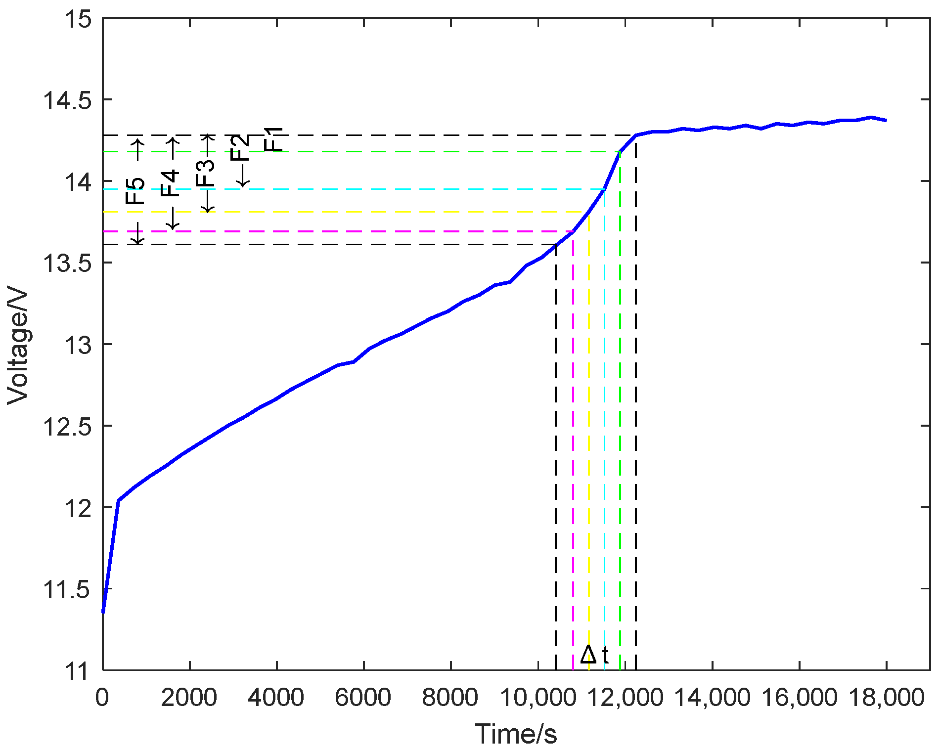
The rest of this paper is organized as follows: In Section 2, the features are extracted from the charging curve, that is, the five equal time voltage differences and the total constant current charging time during the constant current charging period, which are used as the inputs of the SOH estimation model. Section 3 describes the method proposed for SOH prediction, introduces the LSTM network optimized by the improved bat algorithm of Levy flight, and uses the proposed model to complete the prediction of the health status of lead–acid batteries. The experimental results are verified and analyzed in Section 4, and the conclusions about the work described in this paper are given in Section 5.

2. Characteristic Engineering

2.1. Feature Extraction

The most direct parameters of battery aging state are capacity and internal resistance, but capacity and internal resistance are often not easy to measure directly. Generally, starting from the data (current, voltage, temperature, time interval) that can be directly monitored outside the battery, the discharge stage of a lead–acid battery is uncertain and random, while the characteristics of the charging stage are relatively clear. Chuanping lin et al. explained the reason why the duration of some voltage segments on the charging curve played a decisive role in the aging of the battery from a physical point of view and then used several short charging time segments as features to train unlabeled data and poorly labeled data together to build a semi-supervised learning framework and achieved good prediction results [15]. Jinpeng Tian et al. proposed a method to flexibly estimate the health state and charge state of the battery based on deep learning and, by using the charging data sampled in different voltage intervals, a deep neural network (DNN) can be used to predict the complete charging curve and extract effective information about battery degradation [16].

Based on the above analysis, this paper extracts the characteristics of constant current and constant voltage (CCCV) charging stage to analyze and model. The voltage variation curves obtained in different cycle periods are shown in Figure 1. During the charging process of constant current first and then constant voltage, the speed at which the voltage reaches the cut-off charging voltage is significantly accelerated with the increase in the number of cycles, which also means that the difference in charging voltage is different in the same charging time period. This is due to the increase in the number of cycles and the chemical reaction between electrolyte and electrode materials, resulting in capacity attenuation. Therefore, the time for the battery to reach the cut-off voltage is advanced, the constant current charging time will be reduced, and the constant voltage charging time will be increased, that is, the time required for charging will be shortened.

According to the corresponding relationship between the constant current charging time and the current capacity during each cycle of charge and discharge, the relationship curve as shown in Figure 2 is obtained. It is easy to know from Figure 2 that the constant current charging time changes significantly with the capacity attenuation. The time change in constant current charging is consistent with the change trend of capacity. With the increase in cycle times, the constant current charging time becomes shorter.

Figure 3 shows the different voltage differences in the same time range in each cycle as features in the CCCV charging curve. ∆V refers to the voltage difference value in a certain time range before reaching the constant current charging deadline time point, which is called the equal time voltage difference value. We set the fixed time period to t, ∆t ∈ 0.1 h~0.5 h, the voltage difference with an interval of 0.1 h ∆V_0.1h as F1, with an interval of 0.2 h ∆V_0.2h as F2, with an interval of 0.3 h ∆V_0.3h as F3, with an interval of 0.4 h ∆V_0.4h as F4, and with an interval of 0.5 h ∆V_0.5h as F5; the constant current charging time T_cc is set as F6.

2.2. Feature Selection

Feature selection determines the upper limit of the accuracy of the health state estimation model. Feature selection is an important step in the SOH estimation of data-driven methods. In order to further explain the correlation between the selected indirect health factors and battery capacity, the correlation between the indirect health factors and battery capacity was analyzed.

Pearson correlation coefficient can be used to measure the correlation degree between data feature quantities [17]. Pearson correlation coefficient is calculated by the product difference method, based on the dispersion of the two groups of data and their respective average values, and reflects the correlation degree between the two variables by multiplying the two dispersions. The value of the coefficient is always between −1 and 1. Variables close to 0 are regarded as uncorrelated. Variables close to 1 or −1 are regarded as having positive or negative strong correlation. The specific expression is

$$r=\frac{N{\displaystyle \sum XY}-{\displaystyle \sum X}{\displaystyle \sum Y}}{\sqrt{N{\displaystyle \sum X^2}-{\left({\displaystyle \sum X}\right)}^2\sqrt{N{\displaystyle \sum Y^2}-{\left({\displaystyle \sum Y}\right)}^2}}}$$

(2)

where N is the length of the dataset; X and Y represent two sets of eigenvectors.

Grey relational analysis (GRA) is a commonly used method of relational analysis. Its basic idea is to determine the geometric similarity of reference data columns and several comparison data columns to determine whether they are closely linked, which reflects the degree of correlation between curves.

$${\zeta }_i\left(k\right)=\frac{\underset{i}{\min } \underset{k}{\min } \left|x_0(k)-x_i(k)\right|+\rho .\underset{i}{\max } \underset{k}{\max } \left|x_0(k)-x_i(k)\right|}{\left|x_0(k)-x_i(k)\right|+\rho .\underset{i}{\max } \underset{k}{\max } \left|x_0(k)-x_i(k)\right|}$$

(3)

where ρ is called the resolution coefficient, and the value is generally within the range (0, 1) as appropriate.

We calculated Pearson correlation coefficient and GRA respectively for the features F1–F6 mentioned above. According to the definition of Pearson correlation coefficient, the closer the absolute value of the value is to 1, the stronger the correlation is. The closer the value of GRA is to 1, the stronger the correlation is. As shown in

Table 1. Results of the association degree analysis of the characteristics and the SOH.

Features	F1 (∆V0.1h)	F2 (∆V0.2h)	F3 (∆V0.3h)	F4 (∆V0.4h)	F5 (∆V0.5h)	F6 (Tcc)
Pearson	0.7291	0.7624	0.7102	0.6873	0.6690	0.9828
GRA	0.6723	0.7472	0.7794	0.8150	0.8356	0.9693

, the correlation values of the selected six features and SOH are very close to 1, indicating that F1–F6 can be used as the input of the estimation model to achieve accurate SOH estimation.

3. The LSTM Prediction Model Based on the Levy Bat Algorithm

The LevyBA-LSTM SOH estimation model is proposed, using the six features extracted in the previous section as inputs to the LSTM of the model. We also introduce an improved bat algorithm to optimize the parameters of the LSTM network, thereby better achieving the health status assessment of batteries. The following subsections provide a detailed introduction to the construction principles of the model.

3.1. LSTM Evaluation Model

The LSTM model is essentially a specific form of recurrent neural network (RNN). The LSTM model solves the problem of short-term memory in the RNN by adding gates on top of the RNN model [18,19], enabling recurrent neural networks to truly and effectively utilize long-range temporal information. LSTM defines a cell state C_t as an internal memory unit running throughout the entire chain and updates information within the cell state through three gate structures: forgetting gate f_t, input gate i_t, and output gate o_t. The output of LSTM units during time t is calculated by the input i(t), previous state h(t − 1), and C_t, as shown in Equations (4)–(9)

$$f_t=\sigma [W_f·\left(h_{t-1},x_t\right)+b_f]$$

(4)

$$i_t=\sigma [W_i·\left(h_{t-1},x_t\right)+b_i]$$

(5)

$$C_t=\tanh [W_c·\left(h_{t-1},x_t\right)+b_c]$$

(6)

$$C_t=f_t·C_{t-1}+i_t·{\tilde{C}}_t$$

(7)

$$o_t=\sigma [W_o·\left(h_{t-1},x_t\right)+b_o]$$

(8)

$$h_t=o_t·\tanh \left(C_t\right)$$

(9)

where: W_f, W_i, W_c, W_o, b_f, b_i, b_c, b_o are the corresponding weight coefficient matrix and bias terms, respectively; σ, tanh are sigmoid function and hyperbolic tangential activation function, respectively; ${\tilde{C}}_t$ is the standby update content; h_t is the output value of LSTM current moment.

3.2. Bat Algorithm (BA) Based on Levy Flight

The LSTM model not only has a better memory transfer function for long sequence data, but also can eliminate the problem of reverse gradient vanishing. However, during the prediction process, the LSTM neural network model encounters difficulties in adjusting hyperparameters and slow convergence speed. Therefore, a combination of the bat optimization algorithm is proposed to form the BA-LSTM model to optimize LSTM hyperparameters and reduce the impact of difficulties in adjusting hyperparameters and slow convergence speed.

The BA is an effective way to search the global optimal solution by simulating the foraging behavior of a bat. The bat detects the position of prey by echoing the sound pulse, and according to the degree of proximity of prey it adjusts the loudness A, the pulse rate r, and the frequency $f(f\in [f_{\min },f_{\max }])$. Once a target is found, the rate of the pulse is increased and the loudness is decreased, so that the velocity and position are updated to search for the global optimal solution.

Assuming that the foraging space of the bat is a definite-dimensional space, the individual bat in the global search process, the position $X_i^t$, and the velocity $V_i^t$ update formulas are given as:

$$f_i=f_{\min }+(f_{\max }-f_{\min })\beta$$

(10)

$$V_i^t=V_i^{t-1}+(X_i^{t-1}-X^{\ast })f_i$$

(11)

$$X_i^t=X_i^{t-1}+V_i^t$$

(12)

where $\beta \in [0,1]$ is a random vector drawn from a uniform distribution. Here, $X^{\ast }$ is the global optimal solution of the current bat.

For a local search, once each bat has selected a solution from the existing optimal solution, the new solution is generated by a random walk around the optimal solution, which is set as:

$$X_{new}=X_{old}+\epsilon A^t$$

(13)

where $\epsilon$ is the scaling factor, $A^t$ is the average loudness of the total number of iterations for all bats, $X_{old}$ is a random selection of solutions from the current optimal solution.

Update rules of loudness $A_i$ and rate $r_i$: Assuming that as long as the bat finds its prey, the loudness of the pulse decreases and the rate of the pulse increases gradually. The loudness $A_i$ and the rates of pulse $r_i$ are adjusted according to Equations (14) and (15):

$$A_i^{t+i}=\alpha A_i^t$$

(14)

$$r_i^{t+1}=r_i^0[1-\exp (-\gamma t)]$$

(15)

where $r_i^0$ is the initial rate; $\alpha$ and $\gamma$ are constant, generally set to 0.9.

As can be seen from the description of the basic BA, when the bat changes the velocity, the velocity inertia weight is fixed at 1, which leads to a single change in velocity, which is not conducive to the flexible flight of a bat. Considering the experience of the bats themselves, the inertia weight factor $w(t)$ is introduced to increase the flexibility of the bat flight. In addition, in order to improve the performance of the algorithm, a good random Levy flight [12] is introduced in the location update to help the individual bat to jump out of the local optimum.

Based on the above ideas, the velocity update formula of the improved BA is shown as follows:

$$V_i^t=w{(t)}^{\ast }{V}_i^{t-1}+(X_i^t-X^{\ast })f_i$$

(16)

where $w(t)=w_{\min }+i {}^{\ast }(w_{\max }-w_{\min })/T_{\max }$ is the maximum value of w(t), and w_min is the minimum value.

The location update formula is as follows:

$$X_i^t=X_i^{t-1}+V_i^t{}^{\ast }{\mu }^{\ast }sign[rand-0.5]\oplus Levy$$

(17)

where $\mu$ is a uniformly distributed random parameter, the symbol $\oplus$ represents the point multiplication, $rand\in [0,1]$, the random step comes from the Levy distribution.

The bat algorithm of Levy’s flying optimizes the LSTM in the following steps:

Step 1. Initialization parameters: Determine the hyperparameters that the LSTM algorithm needs to optimize, including hidden layer nodes, training times, and initial learning rate; initialize the parameters of the bat algorithm.

Step 2. Data preprocessing: Divide the dataset into training and testing sets, normalize them, and set the output dimensions. Assign vectors in the x, y, and z directions of the bat’s position in the population to the three parameters that the LSTM needs to optimize. Calculate the fitness value of the position vector according to Formula (18), which is:

$$f={\displaystyle \sum _{i=1}^n{\left(y_i^{\prime }-y_i\right)}^2}$$

(18)

where y′_i represents the predicted value of the LSTM model, and y_i represents the expected output value.

Step 3. Updates the bat’s speed and position parameters according to Formulas (16) and (17) to maintain the minimum fitness value.

Step 4. If the maximum number of iterations has not been reached, repeat step 3. If the maximum number of iterations is reached, the optimal parameters are output at this time.

Step 5. Assign the optimized parameters to the LSTM network, train and predict based on these parameters.

The global framework is shown in Figure 4.

4. Experimental Analysis

4.1. Data Description

In this paper, the common charging method is adopted, that is, constant current and then constant voltage, namely CCCV. This charging method is relatively “mild”, which can weaken the impact on the battery and ensure high charging efficiency. The cycle charging and discharge experiments are used to obtain the capacity attenuation curve of the lead–acid battery, while the discharge experiment uses constant current discharge.

The battery pack used in this study consists of 5 tandem single cells with a nominal voltage of 12 V and a nominal capacity of 32 Ah. For a single cell, charging current is 6 A, constant current constant voltage is 14.8 V, discharge current is 10 A, discharge cut-off voltage is 10.5 V. The charging and discharging process settings are: Charging current is 7 A, discharge current is 10 A, charging cut-off voltage is 74 V, discharge cut-off voltage is 52.5 V; charging time is 5 h; test equipment is Xinkehua Capacity & Lifespan Tester (XT05), 60 V–7 A charger, Dekang Battery Charging and Discharging Repair Integrated Tester (SF100-5); ambient temperature is 26 °C.

The experimental steps are: (1) 7 A constant current charging; (2) when the terminal voltage reaches 14.8 V, it switches to constant voltage charging. When the charging time reaches 5 h, the charging phase ends; (3) 10 A constant current discharge, while recording the discharge current and time, calculate the actual capacity using ampere-hour metering method; (4) when the terminal voltage reaches the cut-off voltage of 10.5 V, the charging and discharging cycle ends; (5) repeat steps (1) to (4) 47 times. Analyze the 10,950 sets of data collected during the charging and discharging process mentioned above. These data include recordings of the total voltage, total current, individual battery voltage, charging capacity, and discharge capacity every two minutes.

4.2. Performance Indicators

To comprehensively analyze the effectiveness of the selected method, this article selects the following four indicators to evaluate the performance of the model: Root mean square error (RMSE), mean absolute error (MAE), mean absolute percentage error (MAPE), and decision coefficient (R²). MAE is an absolute error, suitable for situations where there is a significant error between predicted and actual observations, and the MAE is relatively large for larger errors. The smaller the RMSE and MAPE, the higher the prediction accuracy of the model; R² is a comprehensive evaluation indicator that represents the degree of interpretation from data input to result output. The closer R² is to 1, the higher the degree of interpretation. The calculation formulas are as follows:

$$RMSE=\sqrt{\frac{1}{n}{\displaystyle \sum _{i=1}^n{\left(So{H}_i-So{H}_i^{\prime }\right)}^2}}$$

(19)

$$MAE=\frac{1}{n}{\displaystyle \sum _{i=1}^n\left|So{H}_i-So{H}_i^{\prime }\right|}$$

(20)

$$MAPE=\frac{1}{n}{\displaystyle \sum _{i=1}^n\left|\frac{So{H}_i-So{H}_i^{\prime }}{So{H}_i}\right|}$$

(21)

$$R^2=1-\frac{{\displaystyle \sum _{i=1}^n{\left(So{H}_i-So{H}_i^{\prime }\right)}^2}}{{\displaystyle \sum _{i=1}^n{\left(So{H}_i-M_{soh}\right)}^2}}$$

(22)

where SoH_i is the actual measured value, SoH_i′ is the model evaluation value, and n is the number of samples.

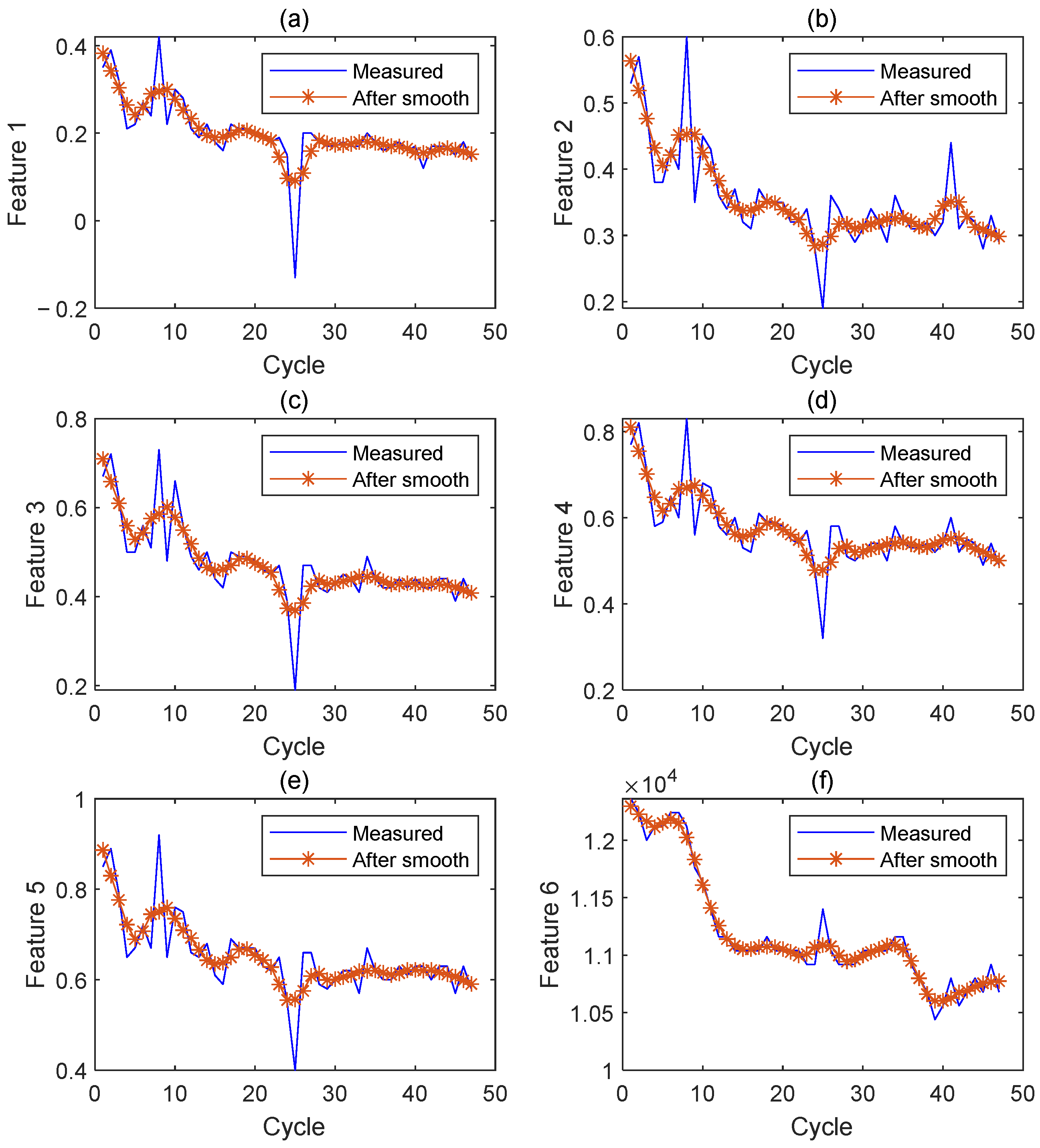
4.3. Data Preprocessing

Data outlier handling: If the outliers in the data deviate significantly from the remaining observed values of the sample, they need to be removed from the sample.

Data normalization processing: To reduce prediction errors, it is necessary to unify the dimensions of parameters before conducting model training and normalize the data to within [0, 1]. The equation is:

$$x_n=\frac{x_m-\min (x)}{\max (x)-\min (x)}$$

(23)

where x_m is the raw data, x_n is the normalized data, and max(x) and min(x) are the maximum and minimum values of the variable x, respectively.

4.4. Model Training

The population size N of the bat optimization algorithm was set to 10 and the maximum number of iterations was set to 10, the individual dimension D was set to 3. The initial parameters of the LSTM model are set as: The number of hidden layers is set to 1, the number of hidden layer cells is set to 200, the number of iterations is set to 20, and the initial learning rate is set to 0.005.

The normalized 6-feature data are used as input to the LevyBA-LSTM model, the structure is $X_n^i=\left\{\Delta V_{0.1h}^i,\Delta V_{0.2h}^i,\Delta V_{0.3h}^i,\Delta V_{0.4h}^i,\Delta V_{0.5h}^i\right\}$, where i represents the number of i-th cycles. The model output is the current actual capacity of the battery C_t. The current SOH is calculated from Equation (1), and the performance index is calculated from Equations (19) to (21). The first 30 cycles of the dataset were used as the training set, and the remaining 17 loops were used as the test set.

4.5. Model Validation

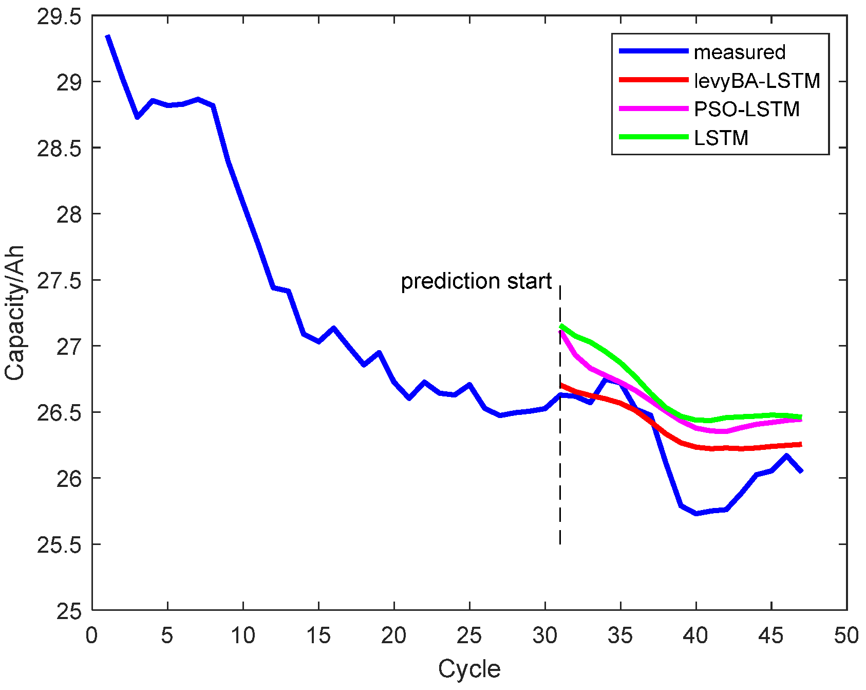
In this paper, the experimental validation was performed in the Matlab R2019b environment. To further illustrate the predictive performance of the LevyBA-LSTM algorithm, this method was compared with the LSTM algorithm and the PSO-LSTM algorithm. For each validation, for a reliable assessment of the error, the model was trained 10 consecutive times, and after completing 10 consecutive training sessions, we took the average of 10 consecutive performance scores for the final performance score.

Figure 5 compares the predicted maximum available capacity of the proposed model with the PSO-LSTM model and the basic LSTM model, and the curves show that the model prediction curve with the number of cycles is consistent with the true trend, which means that the architecture is quite robust. Specific numerical values are presented in

Table 2. Comparison of the SOH prediction performance of each model.

	RMSE	R2	MAE	MAPE (%)
LSTM	0.4962	0.4957	0.4295	1.5862
PSO-LSTM	0.4228	0.8516	0.4467	1.5224
LevyBA-LSTM	0.4389	0.4812	0.3771	1.4468

.

As shown in Table 2, while the PSO-LSTM model performs better on RMSE and R² compared with the LSTM model and the LevyBA-LSTM model, while the LevyBA-LSTM model performs better on MAE and MAPE compared with the LSTM model and the PSO-LSTM model. The MAE of the LevyBA-LSTM model is 0.377 Ah, which indicates that the MAE of SOH is 1.2%, and this accuracy is acceptable in practice.

In order to reduce the measurement noise, the experimental data are smoothed before training prediction. The first 30 cycles of the dataset are used as the training set, and the remaining 17 cycles are used as the test set. Figure 6 shows the comparison of data before and after smoothing. The prediction error results are shown in Figure 7, and the specific prediction values are shown in

Table 3. Comparison of predictive performance after smooth data processing.

	RMSE	R2	MAE	MAPE (%)
LSTM	0.42737	0.77446	0.38990	1.4938
PSO-LSTM	0.41256	0.75377	0.36064	1.3849
LevyBA-LSTM	0.27268	0.84820	0.21609	0.83205

.

As shown in Table 3, after performing smooth preprocessing on the target data, we can find that the proposed LevyBA-LSTM model obtains the smallest RMSE, MAE, and MAPE compared with the LSTM model and PSO-LSTM model. Additionally, the LevyBA-LSTM model obtains the highest R². The MAE of the LevyBA-LSTM model is 0.216 Ah, which indicates that the MAE of SOH is 0.68%, and the prediction performance is 0.5% higher than that without data smoothing. To summarize, based on smoothing preprocessing, the proposed LevyBA-LSTM model exhibits satisfactory performance for SOH estimation on the target dataset.

5. Conclusions

In this paper, the health status of lead–acid battery capacity is the research goal. By extracting the features that can reflect the decline of battery capacity from the charging curve, the life evaluation model of LSTM for a lead–acid battery based on bat algorithm optimization is established. The accuracy of the battery life evaluation model is improved through continuous testing, training, and optimization of the battery evaluation model. In addition, the basic LSTM and PSO-LSTM are constructed for comparison and verification. The experimental results show that the proposed model, especially when the experimental data are smoothed before training and prediction, has better adaptability and prediction accuracy.

Our future work will focus on considering the types and conditions of increasing the training set, so that the model can obtain reliable SOH prediction values for different working conditions. In addition, the prediction method studied in this paper is mainly aimed at the battery state under stable working conditions, and further study of the health state prediction method under loads with relatively large fluctuations is needed.