Abstract
Recently, triple-network convergence systems (TNCS) have emerged from the deep integration of the power grid, transportation networks, and information networks. Fault recovery research in the TNCS is important since this system’s complexity and interactivity can expand the fault’s scale and increase the fault’s impact. Currently, fault recovery focuses primarily on single power grids and cyber–physical systems, but there are certain shortcomings, such as ignoring uncertainties, including generator start-up failures and the occurrence of new faults during recovery, energy supply–demand imbalances leading to system security issues, and communication delays caused by network attacks. In this study, we propose a recovery method based on the improved twin-delayed deep deterministic algorithm (TD3), factoring in the shortcomings of the existing research. Specifically, we establish a TNCS model to analyze interaction mechanisms and design a state matrix to represent the uncertainty changes in the TNCS, a negative reward to reflect the impact of unit start-up failures, a special reward to reflect the impact of communication delay, and an improved actor network update mechanism. Experimental results show that our method obtains the optimal recovery decisions, maximizes restoration benefits in power grid failure scenarios, and demonstrates a strong resilience against communication delays caused by DoS attacks.
1. Introduction
In recent years, the TNCS has emerged due to the rapid development and deep integration of power grids, transportation networks, and information networks caused by the widespread adoption of electric vehicles. This convergence system enables efficient coordination among energy flow, traffic flow, and information flow [1,2]. However, the increasing complexity and interdependence of the system have also created favorable conditions for fault propagation, in which local disturbances can easily initiate cascading failures across networks, resulting in severe system risks such as wide-scale power outages [3,4,5,6,7]; therefore, research on fault recovery method for the TNCS is essential.
The development of a recovery method for the TNCS necessitates a clear understanding of its interaction mechanisms. However, there is a paucity of explicit domestic and international research on modeling the interaction mechanisms of such systems, which adds to the complexity of the study. Furthermore, there is a paucity of research on fault recovery methods related to the TNCS. Despite this, a body of research exists on fault recovery for power grids and power cyber–physical systems. In reference [8], for instance, a cascading fault recovery model based on the sequential recovery graph (SRG) was suggested for power transmission networks and was proven by simulations. In reference [9], an optimization model for the entire black start restoration process in gearbox systems was formulated and solved using a linearized hybrid integer linear programming model and the L-shaped algorithm, taking into consideration the uncertainty of wind power output. Reference [10] analyzed the potential delays caused by information system failures in power system generation, transmission line operation, and load restoration. In these studies, however, the impact of generator start-up failures on restoration decisions was not considered. Reference [11] proposed a parallel recovery method for power systems. Although this method considered uncertainties during the restoration process, it did not consider the possibility of new faults occurring in power systems during component restoration.
The recovery of power system components can result in alterations to the power system’s topology, power flow, and power levels, which may cause problems such as line overloads, imbalances in energy supply and demand in certain regions, and system instability. However, existing research lacks studies on the risks of new faults or system instability that may arise from component recovery. For instance, in reference [12], a two-stage recovery strategy was proposed for power facility restoration after hurricanes, focusing on the design of distributed generation and maintenance personnel scheduling but excluding the analysis of new faults that might occur from power system component recovery. References [13,14,15] also ignored the occurrence of new faults.
It is evident that existing research typically establishes optimization models for different fault scenarios and solves them using various optimization algorithms; however, they lack consideration of uncertainties that may occur during the actual restoration process, such as generator start-up failures and faults triggered by recovery actions, and their impact on recovery decisions. Consequently, these uncertainties should be considered when studying fault recovery methods for TNCS. Such research methods would be more applicable to real-world circumstances.
Moreover, due to the high complexity and interactivity of the TNCS, network attacks can exploit intricate network interaction mechanisms and exacerbate the hazards of faults with relative ease. By manipulating power grid data and injecting false information, for instance, the assessment of the system’s operational status may deviate, resulting in erroneous decisions by administrators and potentially triggering large-scale cascading failures [16,17,18,19]. By injecting a large number of useless requests and obstructing communication channels, DoS attacks can cause an increase in communication delays and, thus, initiate or exacerbate power outages [20,21,22,23,24]. An example of this was the DoS attack launched by a hacker group against a power company in the western United States in 2019, which resulted in communication disruption between the control center and various site devices [25]. There is limited research on restoration decisions for power cyber–physical systems that take network attacks into account at present. While the optimization strategy proposed in [26] considered the impact of information system failures caused by DoS attacks on the restoration process, the solving algorithm lacked the flexibility to handle uncertainty factors and became less efficient as the system scale increased.
The TD3 algorithm, from the discipline of deep reinforcement learning, can be used to address this issue [27]. By appropriately designing the state space and reward function, uncertainties can be accounted for, and the neural network can effectively address the curse of dimensionality problems caused by the large scale of the TNCS [28,29]. In addition, compared to the deep Q-network (DQN), actor–critic (AC), and deep deterministic policy gradient (DDPG) algorithms [30,31,32], the TD3 algorithm exhibits a better capability to suppress network overestimation and provides more stable network training. Consequently, the TD3 algorithm demonstrates significant advantages over existing methods in addressing the complexity of the system’s scale, uncertainties, and stability during the solution process, making it more suitable for solving the model. However, the optimization objective of the TD3 algorithm is to find actions that maximize the action-value function in different states without considering the specific role and impact of recovery actions in particular scenarios, such as system security; therefore, improvements to the TD3 algorithm are necessary to ensure system security.
Based on the above analysis, this study makes the following main contributions to the research on fault recovery methods in TNCS:
- Focusing on the charging behavior of electric vehicles, a TNCS model is established to reveal the underlying interaction mechanisms;
- An efficient fault recovery method for TNCS is proposed, incorporating an improved TD3 algorithm and considering communication delays. By designing and improving the TD3 algorithm, the uncertainties and security issues in the restoration process are considered, leading to the design of an effective recovery algorithm. In addition, the resilience of the algorithm is evaluated by introducing DoS attacks in the context of power grid faults. Lastly, the efficacy of the proposed recovery method is demonstrated through simulation experiments.
2. Methods
2.1. Modeling
The TNCS system comprises three integral components: the power grid, the information network, and the transportation network. Initially, we model the power grid, the scale of which is contingent upon actual demands. Subsequent to this foundation, we construct corresponding transportation and information network models, enabling the circulation of energy and information flows among the three components.
2.1.1. Overall Framework
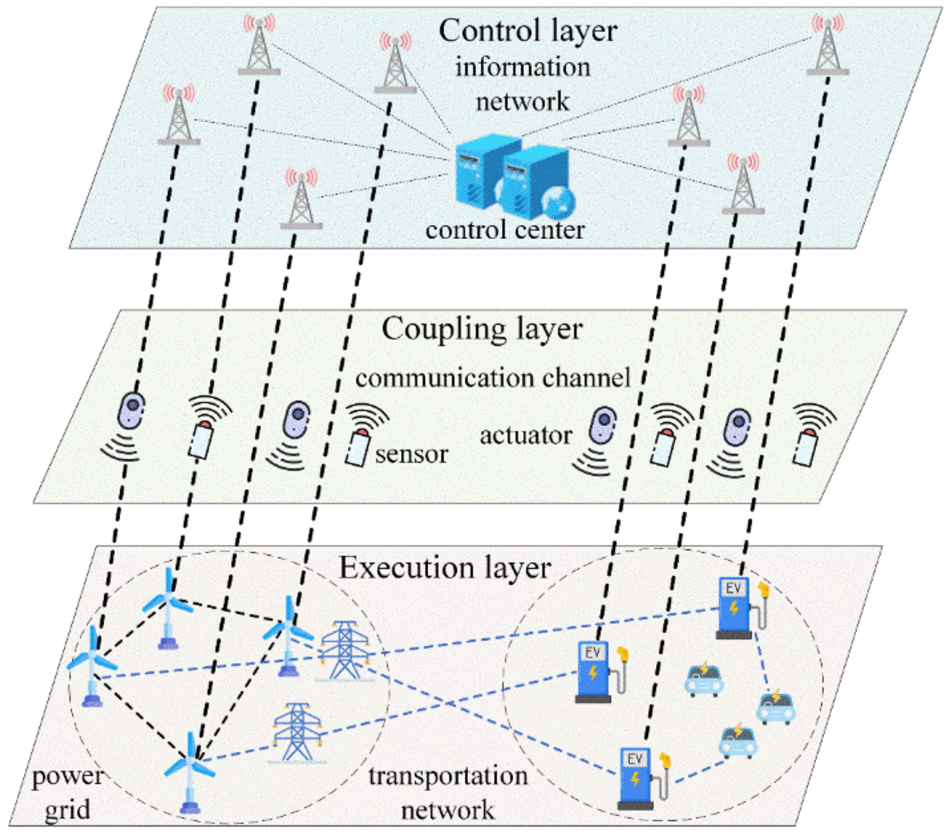
We represent the overall framework of the TNCS system as a whole, consisting of three layers, as shown in Figure 1. The execution layer consists of the actual power grid and transportation network, which is responsible for the reliable operation of energy interactions. The coupling layer mainly consists of power collection and control devices, as well as communication channels, and is responsible for information acquisition, execution of control commands, and information data transmission. The control layer, primarily based on the information network, is responsible for state monitoring and dispatch control.

Figure 1.
The TNCS model. In the power grid, wind turbines are considered as power nodes, supplying energy to charging stations in the transportation network via blue electrical lines. The charging stations, in turn, deliver energy to electric vehicles through blue lines. Operational data from both the turbines and charging stations are relayed to various information nodes in the control layer via thicker black transmission links. Within the information network, we use the base station icon to represent the information nodes, fulfilling the roles of data reception and transmission. Furthermore, while the control center is typically an amalgamation of multiple devices and systems, we employ a computer icon as its symbol for representational simplicity.
Within the execution layer, the power grid continuously powers the transportation network through electrical transmission lines. Their operational parameters are collected by sensor devices in the coupling layer and relayed to the information nodes within the control layer. These nodes aggregate the gathered data into the control center. Subsequently, the directives generated by the control center are conveyed to the physical systems in the execution layer through actuators within the coupling layer.
2.1.2. Execution Layer
The power grid topology is a directed graph, , where represents power nodes, including generators, loads, and circuit breakers, and represents the transmission lines. The topological information for the power grid is represented by a matrix whose elements adhere to the following rules: denotes the presence of a line between nodes i and j, while denotes the absence of a line. The nodal admittance matrix , nodal injection power vector , line power flow vector , and nodal phase angle vector are established. Based on the DC power flow model, the power flow information matrix of the power grid can be obtained from the following equations:
where the value of is and represents a diagonal matrix with vector as its diagonal elements.
The road topology of the transportation network is an undirected graph, , where represents road nodes (including charging stations) and represents paths between them. A matrix is established to represent the topological information of the transportation network, with matrix elements following the rules: indicates the presence of a connected road between road nodes i and j, while indicates the absence of a connected road. A decision vector is used to assess whether each road node has a charging station, where indicates the presence of a charging station in road node i and indicates its absence. A charging station load vector is introduced for the transportation network, where represents the load at the charging station located on road node i and can be obtained from the following equations:
where represents the number of charging piles in the charging station located at road node i. indicates the operational status of the j-th charging pile in the charging station at road node i, with a value of 1 indicating that it is operational and 0 indicating that it is not. represents the operational status of the j-th charging pile in the charging station at road node i, with 1 indicating operation and 0 indicating inactivity. represents the charging power of the j-th charging pile at the road node i charging station.
To ensure the safety of charging services, the maximum charging power for each charging pile must be specified. Establishing a maximum power vector , where represents the maximum charging power of the j-th charging pile in the charging station at road node i.
2.1.3. Coupling Layer
The matrices and are respectively defined to represent sensor deployment in the power grid and transportation network. In , diagonal elements denote sensors on the nodes of the power grid, while off-diagonal elements represent sensors on the power lines. In , the diagonal elements represent sensors on the road node charging stations. The elements of both matrices are assigned the value 1 to denote the presence of a sensor and the value 0 to denote the absence of a sensor. The actuator matrices and are defined in the same way as the sensor matrices.
The uplink data communication channel matrix contains for the power grid and for the transportation network. The matrix elements, , satisfy . In , indicates the presence of an uplink data communication channel between the sensor on the power grid node and the information network control center, transmitting node power information. indicates the existence of an uplink data communication channel between sensors on power grid lines i-j and the information network control center, transmitting current flow information and circuit breaker status. In , denotes the presence of an uplink data communication channel between the sensors in the charging station at road node i and the information network control center, transmitting charging station operational information. The downlink data communication channel matrix is defined in the same way as and , with different transmitted content. It carries commands for the charging station’s circuit breaker open or close, node power adjustment, charging pile open or close, and maximal charging power adjustment.
2.1.4. Control Layer
The information network topology is defined as a directed graph, , where represents the information nodes and represents the communication links between nodes. The connectivity status of the communication links is represented by the link status matrix , with matrix elements . A value of indicates that an effective connection has been established between information nodes i and j. The control center in the information network adjusts the operational status of the power grid and transportation network based on the received data. The storage of received information includes and for power flow information () and power grid topology information (), respectively, while represents the storage of received charging station information. Utilizing this information, the reduction in output of generator nodes and the reduction in load of load nodes are calculated, thereby calculating the decrease in power at the charging stations in the transportation network, as illustrated below:
where satisfies Equations (1)–(3), and is used to represent the reduction in output of power nodes or the reduction in load of load nodes. is the drop value in charging power at road node i, while is the adjusted average charging power of the charging piles in the charging stations. refers to the adjusted operational state of the j-th charging pile in the i-th road node. N represents the number of road nodes in the transportation network. We assume that the charging stations will bear the maximum extent of power grid load variations.
The control center then generates and distributes decision instructions to the executive layer.
2.2. Fault Recovery Method
Common power grid failures often arise from localized disturbances or anomalies, subsequently spreading and affecting the operational status of other lines or nodes, potentially leading to a system-wide collapse, which is referred to as cascading failures. Cascading failures have a more pronounced impact and are more frequently encountered in real-life scenarios; consequently, our design of fault recovery methods primarily targets multi-fault situations.
2.2.1. Design of Restoration Model
In this section, we define important indicators for power grid faults in the context of the TNCS, assessing the importance of faulty power lines. With the objective of maximizing restoration benefits, a restoration model is established.
We assume that power grid faults in the TNCS result from the overload-induced disconnection of power lines, leading to the redistribution of power flow, reduction in output of generator nodes, and load shedding at load nodes. Concurrently, adjustments are made to the charging power of the charging stations in the transportation network corresponding to the affected power nodes, which may impact the travel of EV users. The importance of power lines, , is determined by the importance of its connected power nodes () and the importance of the charging stations on the corresponding coupled road nodes (), as shown below.
where represents the weight coefficient. and are binary variables that indicate the existence of the respective item, taking a value of 1 if it exists and 0 otherwise. consists of the degree, generation capacity, and load of the power nodes and consists of the degree of the road nodes and the number of electric vehicles affected, as shown below:
where , , , , and are binary variables indicating the existence of the respective items. represents the power output of generator nodes and represents the total power output of generator nodes. represents the degree of nodes in the power grid, while represents the sum of the degree of power nodes. represents the degree of road nodes in the transportation network, while is the sum of the degree of road nodes. represents the power load of the load nodes in the power grid, while denotes the total power load of the load nodes in the power grid. obtained by Equations (11)–(13) represents the number of EVs impacted during travel, while represents the total number of EVs impacted during travel. Equation (12) calculates the adjusted number of charging station users , while Equation (13) calculates the adjusted number of charging station electric vehicles . represents the power adjustment matrix for the i-th charging station, represents the identifier of the current charging station users, and represents the identifier of the current charging station reservation users.
After calculating the importance of each power line, they are sorted in descending order to determine the restoration priority. is defined as the quantified priority value, and represents the number of restoration steps. The optimization objective is to maximize the restoration benefit, which consists of the recovery power from the power grid and transportation network, based on the importance of the power lines.
where represents the restoration benefit obtained from restoring the fault at step m. is the active power of the generator, and is the voltage at the terminals of the power system. Equation (20) represents the line flow constraint, where power flow varies with the restoration of the faults. Exceeding the limits of line flow, or , may result in overload issues, leading to the disconnection or damage of the concerned line or other lines. In Equation (21), represents the unit start-up time, while represents the maximum start-up time of the unit, ensuring the required time for thermal start-up. Equation (22) represents the energy supply–demand balance constraint in the power grid, ensuring the balance between actual supply and demand. Imbalances can lead to voltage fluctuations, frequency deviations, and overloaded operation, causing power equipment failures or system security issues such as a power grid collapse. In this study, we assume that energy imbalance can cause line overloads and disconnection so that the fault recovery should avoid energy supply–demand imbalances.
2.2.2. Design of Restoration Algorithm
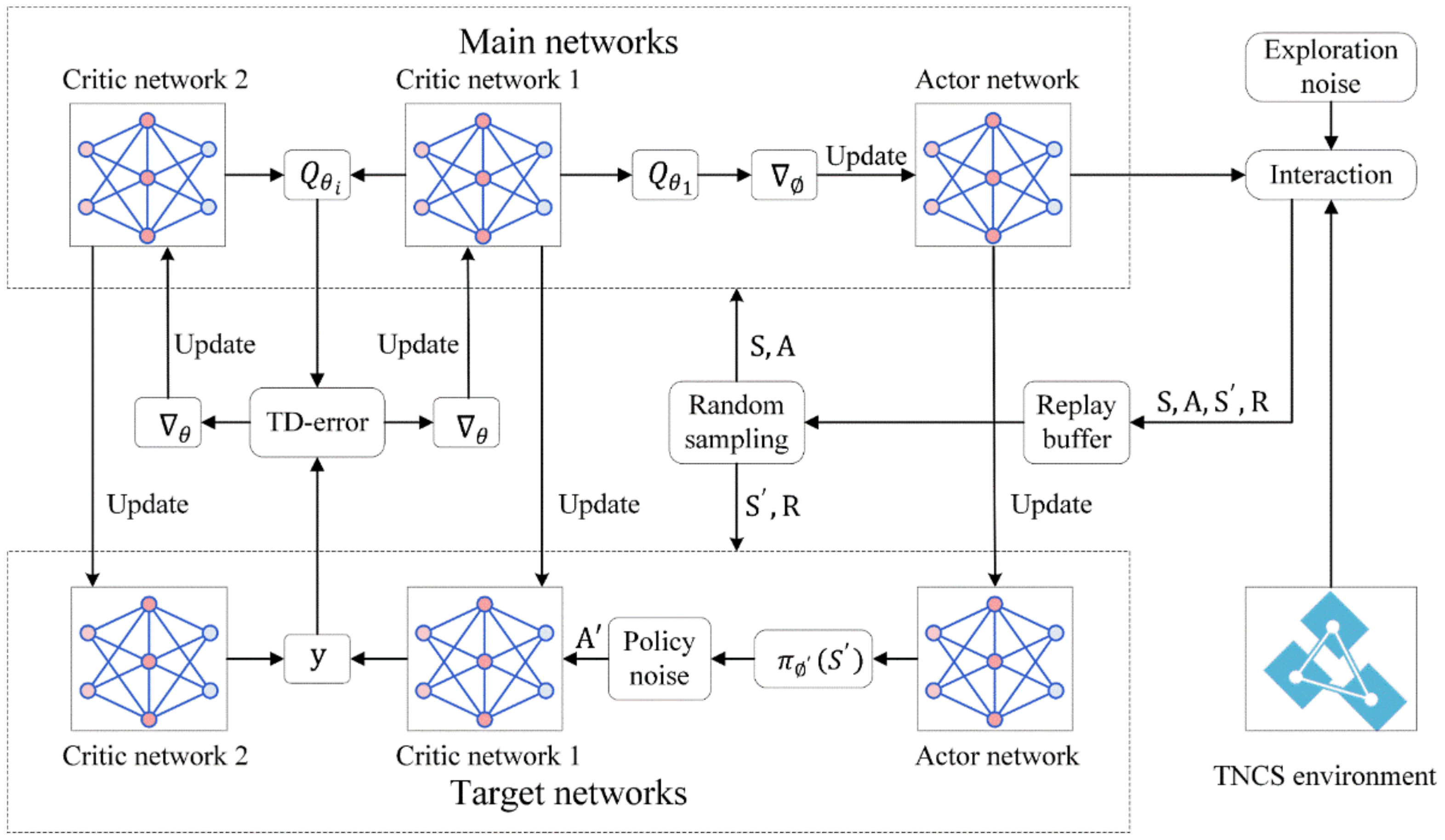
In the context of fault recovery in the power grid of TNCS, the restoration sequence of each faulty line significantly influences the restoration benefit, giving rise to a decision-making problem. In this section, we focus on the design and improvement of the TD3 algorithm in the field of deep reinforcement learning with the aim of determining the optimal restoration strategy. Figure 2 illustrates the restoration algorithm structure based on the TNCS.
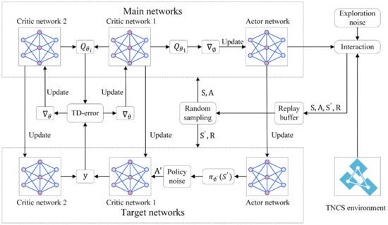
Figure 2.
Structure of the restoration algorithm. First, the TNCS environment interacts with the actor network in the main networks, incorporating exploration noise. Specifically, this interaction indicates the state matrix , as the input to the actor network, and the actor network chooses an action based on . Then, the action can change the state matrix, resulting in a certain reward. Second, the obtained transitions from the interaction (transitions primarily include , , and ) are preserved in the replay buffer via experience replay. To train and update the actor network and critic network in the main networks, a batch-sized transition sample is selected at random. During the update of the critic network, a TD-error is generated and gradient descent is performed while introducing policy noise into the process. The actor network is updated using gradient ascent to maximize . The Target networks are updated after a certain number of updates to the main networks.
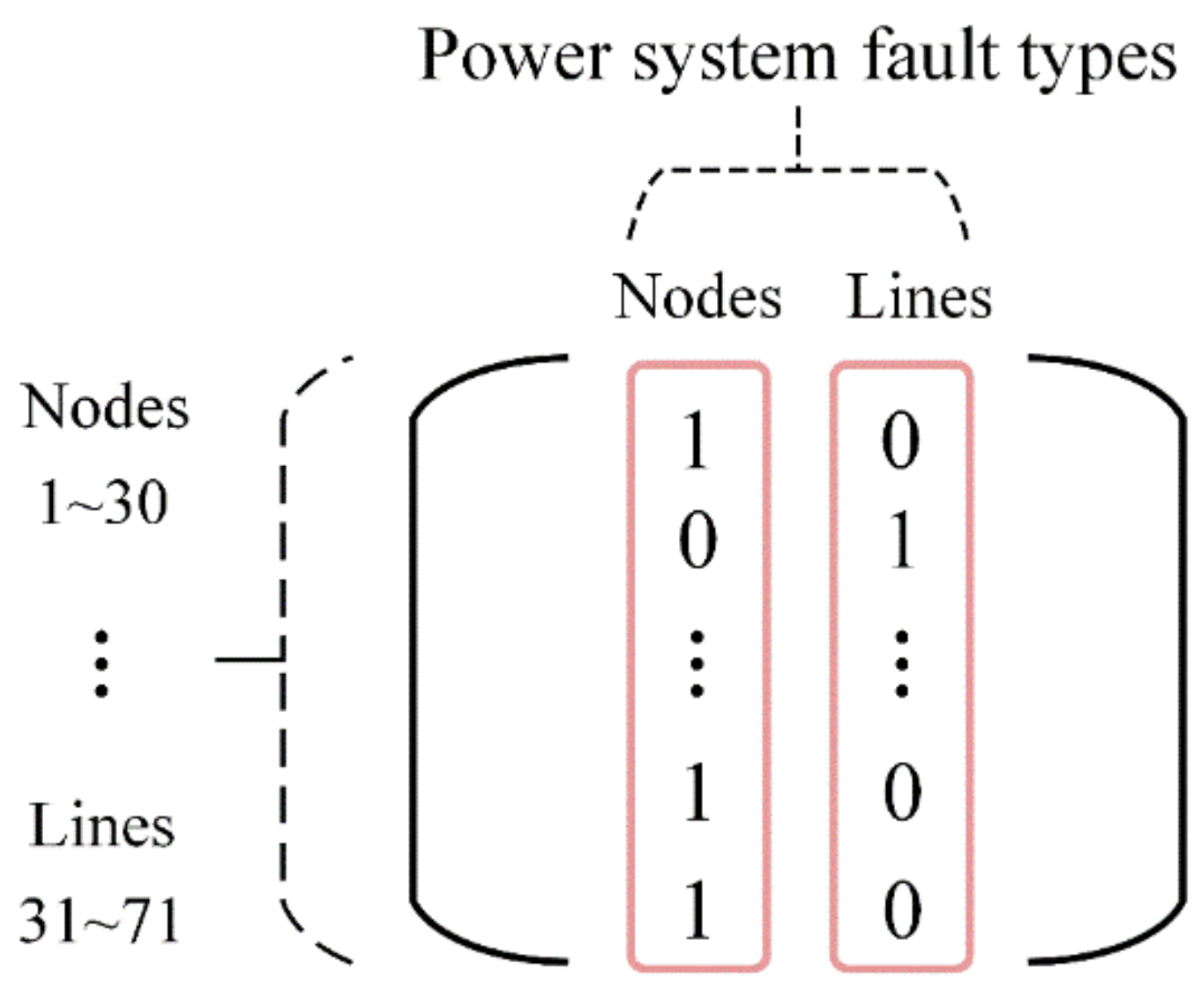
Specifically, we consider the control center as the agent and define the action space as the set of all available restoration actions from which the control center can choose in the TNCS environment, denoted as , and action belongs to . In the restoration model, the recovery of faults can cause new faults. To address this uncertainty, we employ a state matrix to represent the state space, reflecting the changes in the state of the TNCS. As shown in Figure 3, each row of the state matrix represents a power node or line, and each column represents a fault type. The arrangement follows the order of power node and line numbering, as well as fault type. Based on the rows and columns, the location and type of faults can be determined. An element value of 1 indicates no fault, while 0 indicates that a fault exists. Consequently, the changes in the state of the TNCS caused by fault recovery and occurrence can be reflected through the variation of element values.

Figure 3.
State matrix. We assume the presence of 30 power nodes, 41 lines, and fault types including faults at power nodes and lines.
The design of the reward function is as follows:
The control center conducts a status check on the TNCS at the beginning of each restoration step, and when the check is complete, the reward is obtained. If no data information is received from a node or line in the execution layer within time , it is considered communication delays, is set, and the reward is obtained. Equation (25) represents the impact of communication delays on restoration decisions, where and are proportional coefficients with respective ranges of [0,1] and (0,1). represents the total number of restoration stages, indicating the duration of the entire restoration process, while represents the restoration stage at which the communication delay occurs. The restoration stage represents the maximum number of restoration steps required to address communication faults (with a single stage consisting of multiple consecutive restoration steps) and represents the actual number of restoration steps required for communication fault recovery. denotes normal communication, with indicating the effectiveness of the restoration action, resulting in the reward , and the restoration benefit calculated from Equation (24). When equals zero, the restoration action is ineffective, resulting in a negative reward of −1.
The effectiveness of a restoration action refers to its objective of targeting the faulty lines without causing any additional faults. Restoring a power node requires at least one connected power line to be operational (excluding black-start nodes). For a power generation node, Equation (21) must be satisfied, and if not, it is considered a failed unit start-up, which is uncertain and may be caused by unpredictable factors. In the case of a failed unit start-up, the reward function returns −1, reflecting the impact of this uncertainty on restoration decisions, and we can enhance the practicality of our method by employing this approach.
In response to potential system security issues caused by an imbalance between energy supply and demand during the restoration process, the TD3 algorithm is improved as follows:
Equation (27) adds a multiplicative term in the original estimated value used for updating the actor network, where represents the improved estimated value and belongs to the set . represents the set of line importance, as determined by Equation (26). is a binary variable with values of 0 and 1, and it is set to 1 if the restoration action causes an energy supply–demand imbalance in the system and 0 otherwise.
The addition of the multiplicative term can affect the original estimated value after the improvement. When high-priority lines are disconnected due to an energy supply–demand imbalance, the multiplicative term becomes smaller, resulting in a decrease in estimated value and indicating that the restoration actions under the current state pose a security risk to the system. Therefore, the actor network can conclude that the chosen restoration action is not optimal.
Lastly, the neural networks used in the algorithm consist of an input layer, fully connected hidden layers, and an output layer. The specific parameter setting depends on the simulation experimental scenarios.
3. Experiments and Results
3.1. Experimental Settings
Based on the TNCS model, a simulation experimental scenario is constructed as follows.
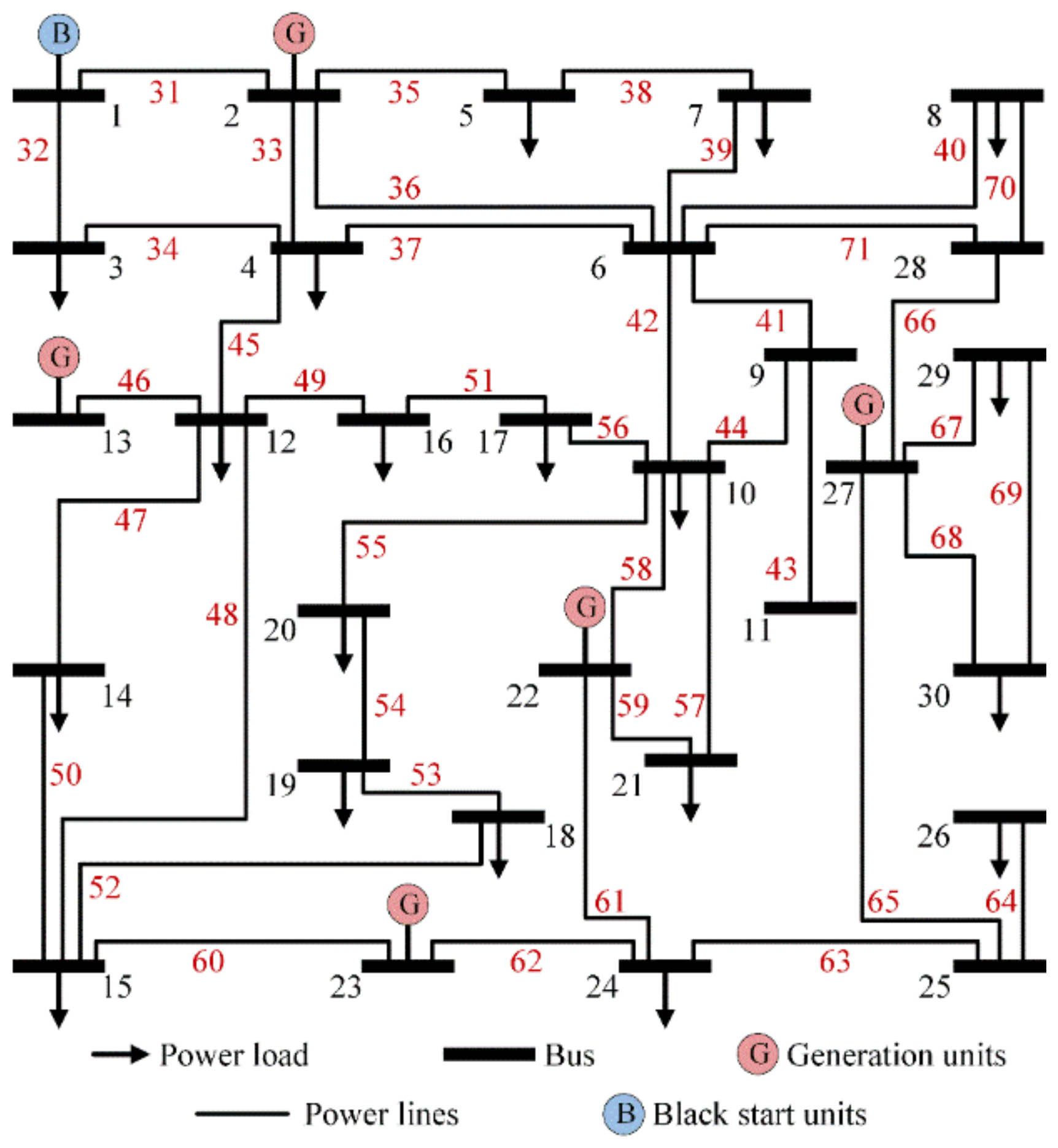
The power grid uses the IEEE 30-bus power system [33], as shown in Figure 4. The transportation network has 5000 EVs and 30 nodes with 50 charging piles at each road node. Each charging pile has a maximal output of 20 kW. The nodes of the transportation network and the power grid with the same number are coupled. The information network consists of 101 information nodes, where the first 30 nodes correspond to the power grid nodes, with node 10 serving as the control center. Nodes 31 to 71 correspond to the power lines, while the remaining nodes correspond to the transportation network nodes. The simulation experiments are implemented using MATLAB programming without GPU acceleration techniques.
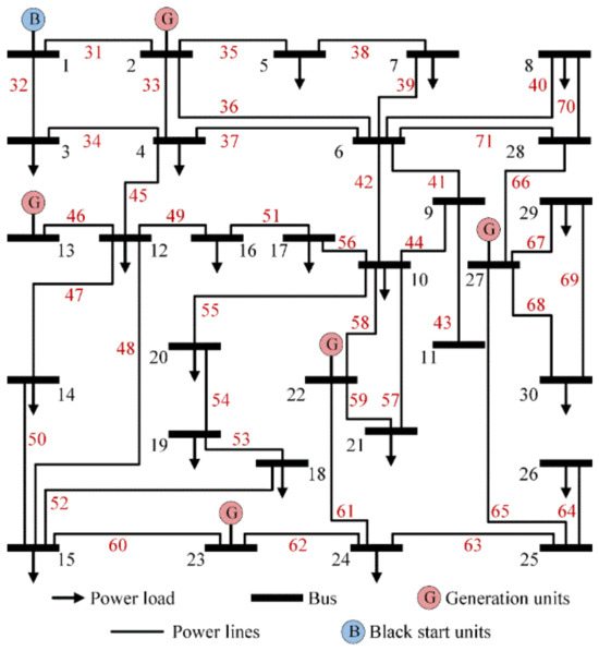
Figure 4.
IEEE 30-bus power system diagram. The power lines are numbered from 31 to 71.
3.2. Small-Scale Power Grid Faults
In this section, we simulated small-scale faults in the power grid of the TNCS. Specifically, we induce faults in the power lines with line numbers 31, 32, 33, 34, 36, and 37, and these lines are placed in an open-circuit state. The specific experimental parameter settings are as follows.
The actor network consists of an input layer with 142 neurons, a first hidden layer with 256 neurons, a second hidden layer with 128 neurons, and an output layer with 6 neurons. The target actor network is updated once after every five updates of the actor network.
The critic network consists of an input layer with 142 neurons, a first hidden layer with 256 neurons, a second hidden layer with 256 neurons, and an output layer with 1 neuron. The target critic network is updated once after every five updates of the critic network.
The ReLU function is used as the activation function in the hidden layers of all networks. The actor network is updated once after every three updates of the critic network. Set the discount factor to 0.99, the exploration noise standard deviation to 0.15, the policy noise standard deviation to 0.3, the batch size to 64, the total number of episodes to 1000, and the , , , and values to 0.5, 0.1, 0.1, and 0.005, respectively. The parameter , specifically, is used in the soft update.
The simulation experimental results are as follows.
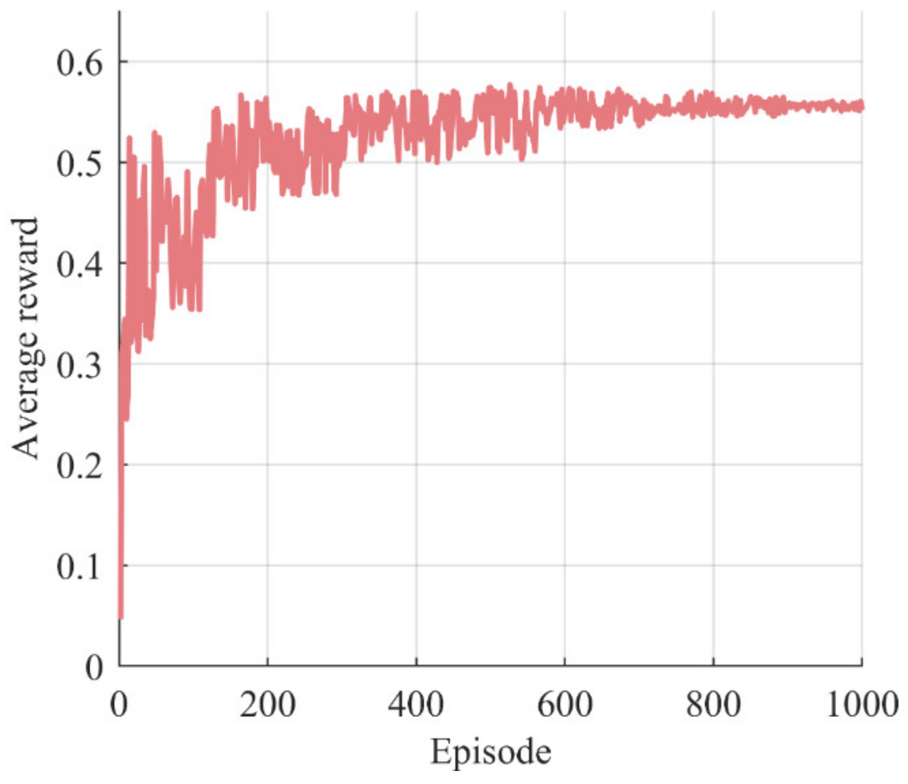
The result in Figure 5 indicates that the actor network is well-trained and able to make accurate and effective decisions.

Figure 5.
Learning curve. We can observe that the learning curve exhibits significant fluctuations during the first 300 or so episodes. Approximately between 300 and 700 episodes, the fluctuations decrease. After roughly 700 episodes, the average reward converges on a stable value.
The obtained restoration scheme is shown in Table 1. The restoration sequence is primarily determined by the order of line restoration; once a line is restored, the connected nodes automatically begin their restoration process (except for black-start nodes). The restoration sequence refers specifically to the order of initiating restoration. As a result, the restoration processes for multiple faults can proceed simultaneously. For example, the restoration of line 36 can be initiated during the restoration of node 1.

Table 1.
Restoration sequence.
To validate the optimality of the restoration sequence, we compared it with several backup schemes (utilizing a solver for computation) based on the restoration benefit criterion. As shown in Table 2, the restoration benefit obtained by our proposed scheme, denoted , was from 15.36% to 25.52% greater than that of the other schemes, indicating that our scheme is optimal in terms of restoration benefit.
Table 2.
Comparison of schemes.
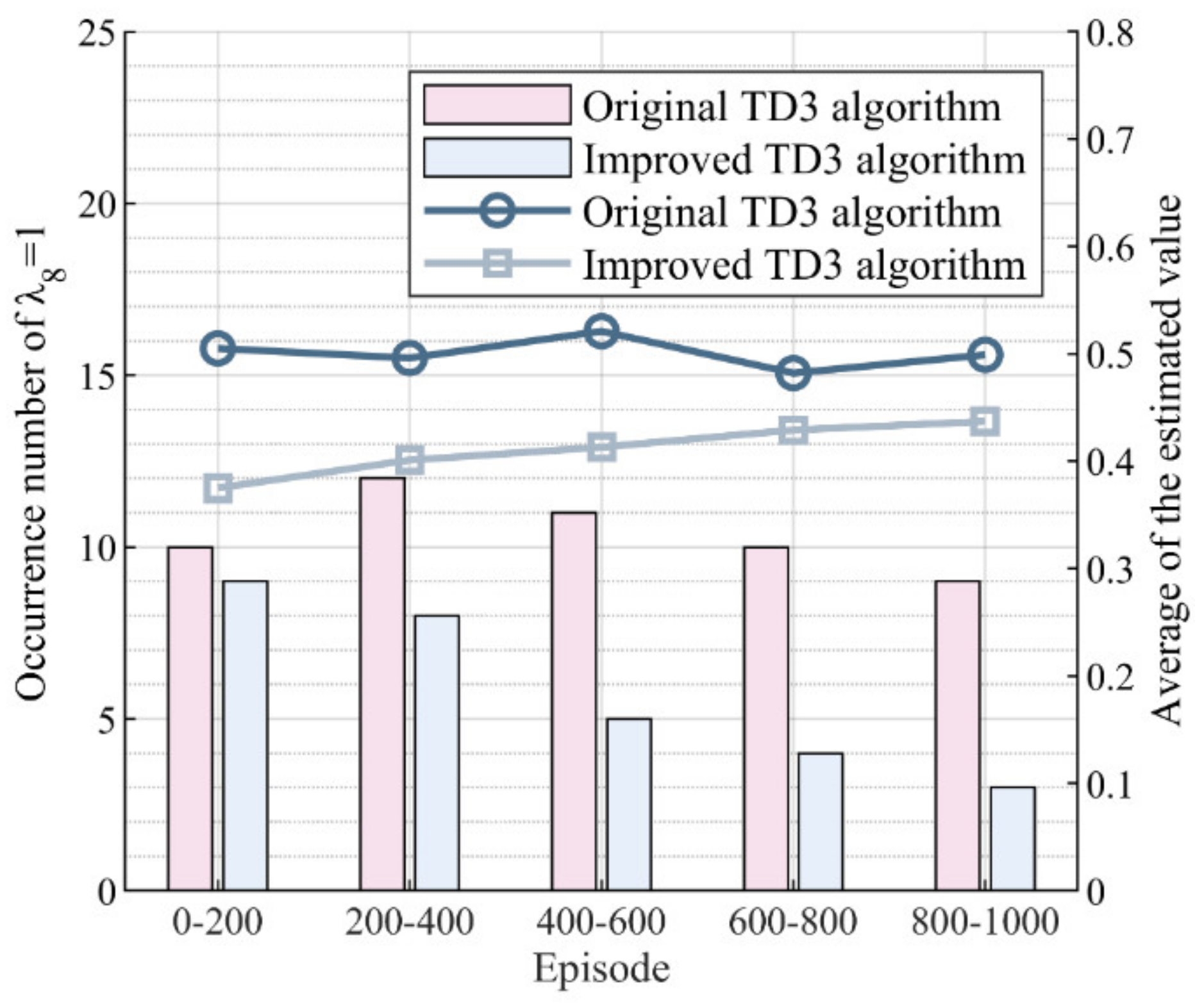
Additionally, Figure 6 shows the improvement effect of the TD3 algorithm.
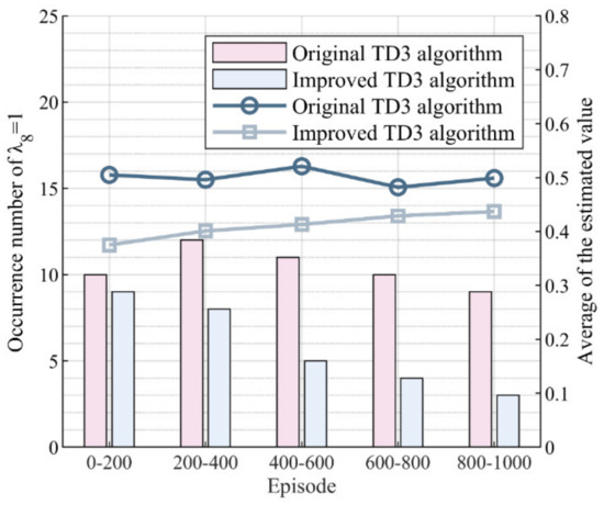
Figure 6.
Improvement effect of the TD3 algorithm. The values of the bar indicate the number of occurrences of per 200 episodes, while the values of the line indicate the average of the estimated value every 200 episodes.
It can be observed that the occurrence number of was lower in the improved algorithm compared to the unimproved version. This indicates that the evaluation of restoration actions in the improved algorithm was not solely based on maximizing , but also considered system security issues caused by energy supply–demand imbalances, as represented by the inclusion of a multiplicative term. Using this method, it is possible to lower the original estimated values , as shown by the lower values of the line in the figure for the improved TD3 algorithm compared to the unimproved TD3 algorithm. When the chosen restoration action leads to an energy supply–demand imbalance, equals 1, the estimated value decreases, and the actor network receives feedback indicating that the chosen restoration action is not optimal. As the number of episodes increases, the actor network gradually learns to avoid restoration actions that may cause energy supply–demand imbalances. Consequently, in the figure, we can observe that the frequency of decreased over time, with only three occurrences between episodes 800 and 1000, representing a probability of 1.5%. This is a 66.67% reduction compared to the unimproved TD3 algorithm, and demonstrates the effectiveness of our improvements to the TD3 algorithm in reducing the probability of system security issues caused by energy supply–demand imbalances during the restoration process.
3.3. Large-Scale Power Grid Faults
We set all power lines to an open-circuit state, paralyzing the power grid in the TNCS. In this scenario, the impact of uncertainties such as failed unit start-up and the occurrence of new faults caused by the restoration process is analyzed, and the algorithm proposed in this study is compared with other algorithms to evaluate the performance and efficacy.
Set the batch size to 128 and the total number of episodes to 5000, while the settings of the remaining experimental parameters are identical to those in the small-scale fault scenario. The simulation results are shown below.
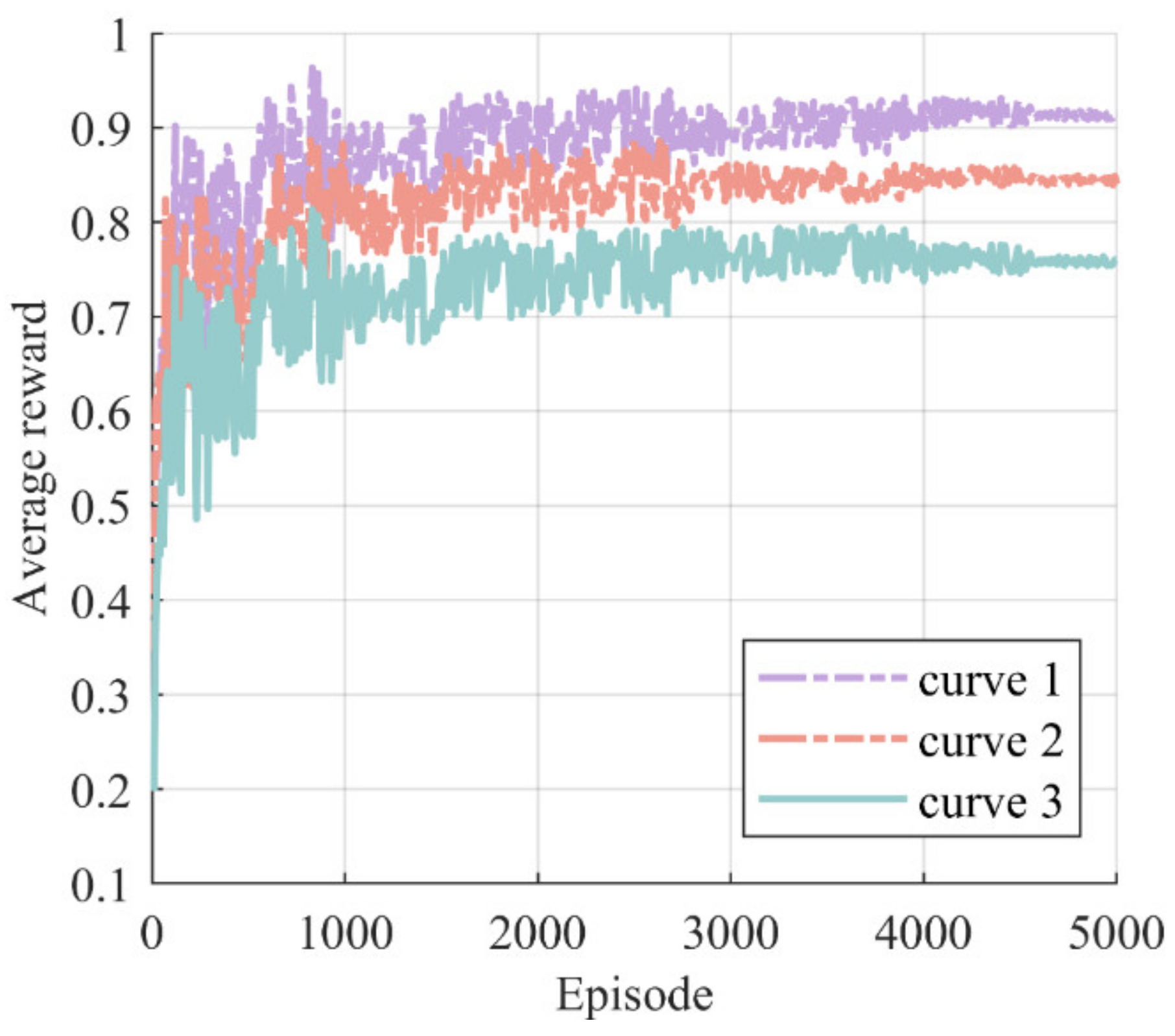
We can observe that curve 3 gradually converged to a stable value in Figure 7, indicating that the actor network was well-trained and able to make accurate and effective decisions in large-scale power grid faults. Furthermore, the three curves showed different average rewards and fluctuations. Curve 3 exhibited the lowest average reward, and curve 3 and curve 1 showed significantly higher fluctuation than curve 2. This is due to the fact that both generator start-up failures and new faults occurring during the restoration process result in a reward value of −1. Consequently, curve 3 exhibited lower values than the other two curves. The presence of new faults increased the uncertain change of and the difficulty of convergence, leading to higher fluctuations in curve 3 and curve 1.

Figure 7.
The impact of uncertainty factors on fault recovery. Curve 1 represents the scenario without considering the possibility of unit start-up failures during the restoration process. Curve 2 represents the scenario without considering the possibility of fault recovery causing new faults. Curve 3 represents the scenario that considers both unit start-up failures and the occurrence of new faults during the restoration process.
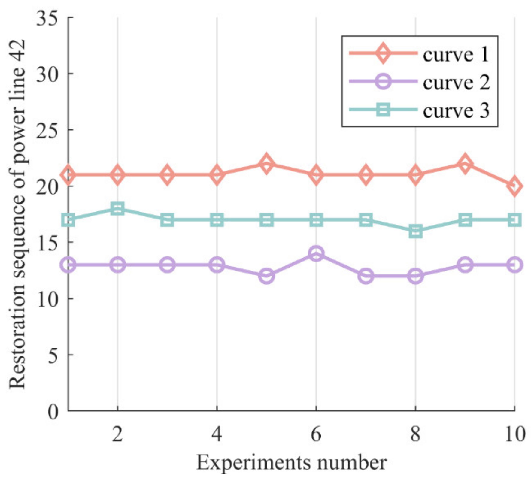
To validate the impact of uncertainties on the restoration sequence, we take the restoration sequence of power line 42 as an example to observe the change of its restoration sequence, and the results are shown in Figure 8. We can observe that in the case corresponding to curve 3, the restoration sequence of power line 42 in 10 experiments was approximately the 17th step, which differs from the cases corresponding to curves 1 and 2. This indicates that uncertainties during the restoration process can alter the restoration sequence and should not be ignored in the practical restoration process.
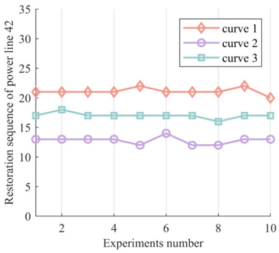
Figure 8.
Impact of uncertainties on restoration sequence. The curves labeled as curve 1, curve 2, and curve 3 in this figure correspond to curve 2, curve 1, and curve 3 in Figure 7, respectively. The restoration sequence of power line 42 refers to the step at which this line is recovered.
At the end of this section, we also compare the proposed algorithm with other intelligent algorithms such as particle swarm optimization (PSO), genetic algorithm (GA), and other deep reinforcement learning algorithms to verify the superiority of the proposed algorithm in solving the fault recovery problem of the TNCS [34,35]. The results are shown in Table 3. We can observe that the proposed algorithm outperformed other algorithms by 0.3% to 20.96% in terms of restoration benefit, and in terms of convergence time, there existed a reduction of 2.82% to 14.39% compared to other algorithms except for the PSO algorithm, with only a marginal increase of 1.2% compared to the PSO algorithm. The aforementioned comparative results demonstrate that the proposed algorithm has distinct advantages in terms of both restoration benefit and convergence time, indicating its superiority in an overall assessment. Moreover, compared to the TD3 algorithm, although the restoration benefit is very close, the proposed algorithm exhibited an 8.93% reduction in time. This is due to improvements made to the TD3 algorithm, which reduces the occurrence of new faults during the restoration process and effectively reduces the uncertain change of , thereby reducing convergence difficulties during training.
Table 3.
Comparison of different algorithms.
3.4. Communication Faults
In this section, we add the simulation of communication faults on the basis of large-scale power grid faults to validate the resilience of the algorithm proposed in this study.
Specifically, we assume that DoS attackers send a significant volume of disguised packets to information nodes 31, 32, 33, and 34, resulting in their infection. As a result, the communication channels within the coupling layer connected to the information nodes and the communication links within the information network of the control layer become blocked. When communication delays are detected, the technical staff at the control center suspend the restoration of power grid faults and initiate the deployment of firewalls and intrusion detection systems to restore the communication faults. Equation (25) demonstrates that the impact of communication delays on restoration benefit depends on its occurrence timing and restoration speed. To facilitate the statistical analysis, the occurrence time of communication delays is divided into six stages: stage 1: 1 to 6 steps; stage 2: 7 to 12 steps; stage 3: 13 to 18 steps; stage 4: 19 to 24 steps; stage 5: 25 to 30 steps; and stage 6: more than 30 steps. We set , with corresponding to the first stage, corresponding to the second stage, etc. There are five levels of restoration speed: level 1: ; level 2: ; level 3: ; level 4: ; and level 5: . Among them, indicates that the restoration of communication delay requires one step, requires two steps, etc. We set and . The remaining experimental parameters are maintained in accordance with the previous section. The simulation results are shown as follows.
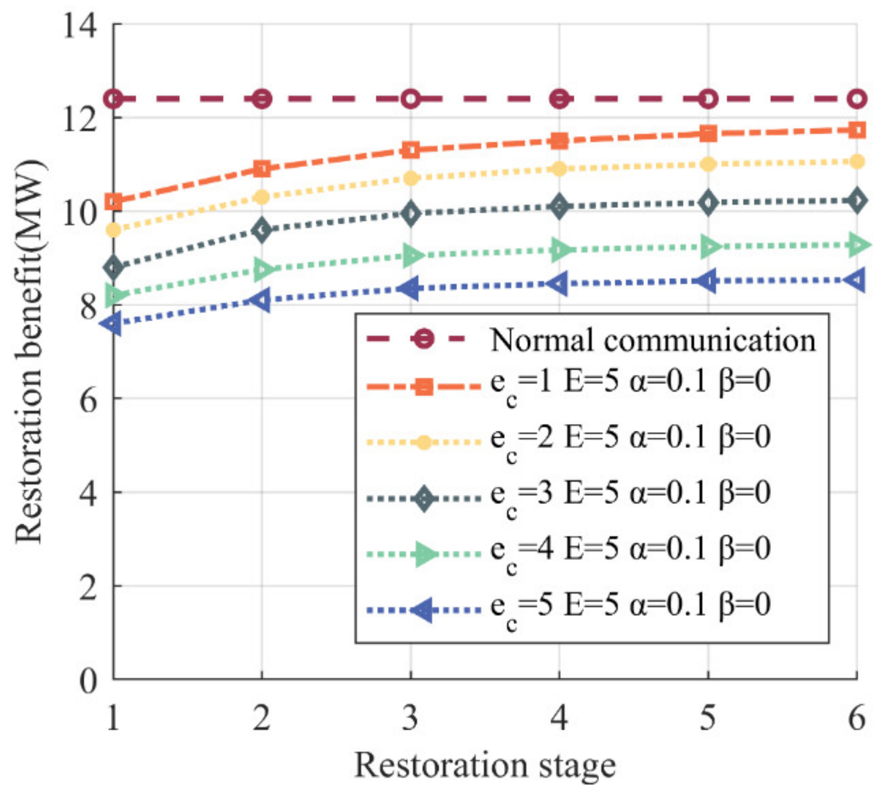
As shown in Figure 9, the restoration benefit of the communication delay curves was less than that of the normal communication curve, which was due to the communication delay causing a reduction in the value of certain power lines, illustrated in Figure 10.

Figure 9.
Impact of communication delays on restoration benefits. There is one curve representing normal communication, the value of which remains constant at 12,3968 MW, and five curves representing communication delay.
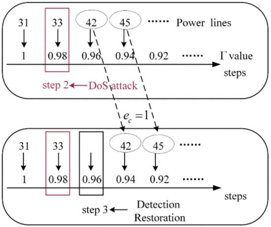
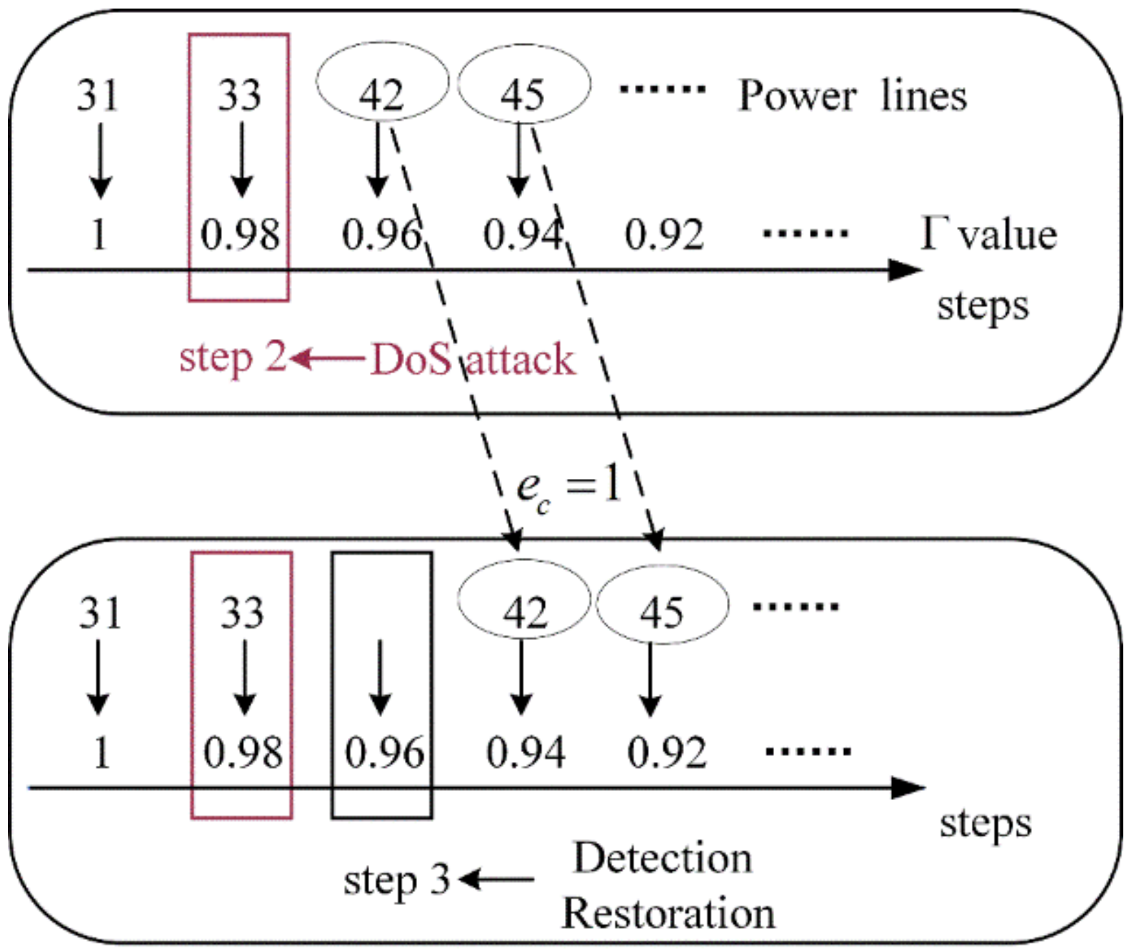
Figure 10.
Mechanism of the value reduction. We assume that a DoS attack is launched against the information node at step 2. It can be observed that the DoS attack has no impact on the restoration of steps 2 and 1. As the restoration process reaches step 3, the control center performs a status check and detects the communication delay, initiating its restoration. Power line 42 cannot be restored in step 3, and its recovery order is changed from step 3 to step 4. The reason it is changed to step 4, rather than step 5, step 6, etc., is because . Similarly, the restoration step for power line 45 transitions from step 4 to step 5, etc. At step 4, regardless of whether power lines 45 or 42 are restored, the value corresponding to step 4 remains unchanged. When power line 42 is restored at step 4, the value reduces from 0.96 (corresponding to step 3) to 0.94. The above analysis explains the reduction of the value.
Figure 9 also illustrates two additional aspects: first is the impact of the occurrence time of DoS attacks on restoration, and second is the impact of restoration speed of communication delay on restoration.
For the first aspect, we can observe that when the restoration speed remained constant, the later the occurrence of communication delay caused by DoS attacks, and less of the restoration benefit was reduced. This is due to the fact that a delayed occurrence of communication delay results in fewer affected power lines, resulting in less reduction in the value of the objective function (as explained by the mechanism for value reduction), while the value remains unchanged. Consequently, the communication delay curve exhibits an increasing trend as the restoration process progresses.
The timing of DoS attacks is characterized by uncertainty, while the reduction in restoration benefit caused by DoS attacks can be mitigated by adjusting the value of . According to Table 4, when the communication delay occurs in stage 1, stage 2, and stage 3, setting to its maximum value of 1 minimizes the reduction in restoration benefit by 9.23%, 4.22%, and 0.68%, respectively, compared to the normal communication benefit of 12.3968 MW. However, in stage 4, setting to 1 leads to a restoration benefit of 12.510 MW, which is higher than the normal benefit and unrealistic. Therefore, cannot be set to 1, and results in a restoration benefit of 12,267 MW, which is marginally less than 12,3968 MW. Thus, the valid range for in stage 4 is . Similarly, in stage 5 and stage 6, the valid range for is and , respectively.
Table 4.
The impact of on restoration benefit.
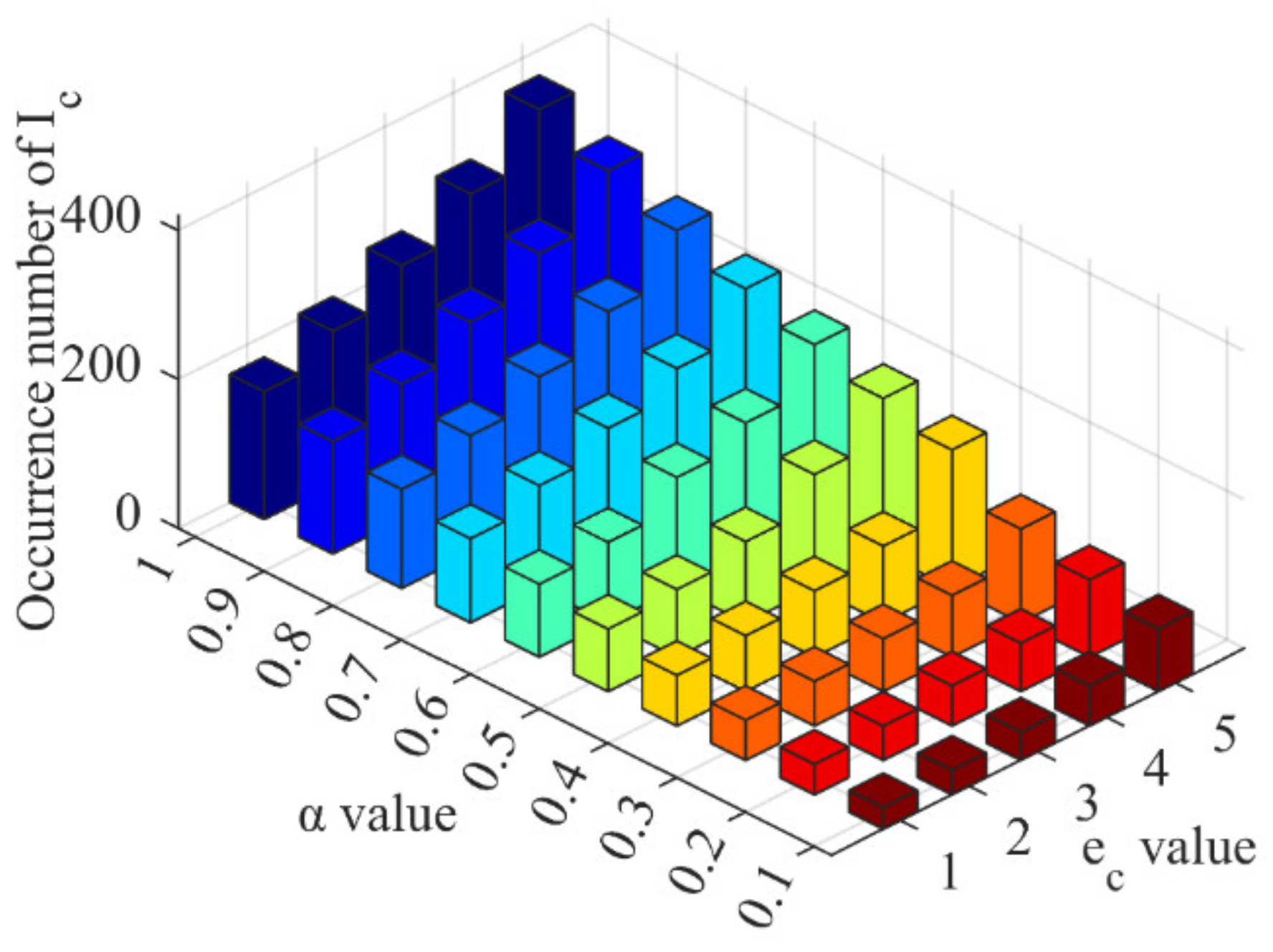
For the second aspect, it can be observed that the restoration benefit of the communication delay curve corresponding to was greater than that of the curves corresponding to other restoration speeds in all restoration stages. This is due to restoring communication delay leading to obtaining the reward . If the restoration speed is fast, such as completing the restoration in a single step, one is obtained. Alternatively, multiple can be obtained if the restoration speed is slow and requires multiple stages to complete. However, and are not equivalent, and a difference exists between them. Obtaining multiple can lead to overestimation or underestimation of , which may result in policy bias and affect restoration decision-making. To solve this issue, we can adjust the values of and to reduce the difference between and . It is important to note that we cannot directly control the restoration speed due to its uncertainty and dependence on the defensive deployment level of the information network. When the occurrence time of DoS attacks is fixed, we can adjust the value of to mitigate the policy bias caused by restoration speed. Figure 11 illustrates the impact of different values of on policy bias when .

Figure 11.
The impact of on policy bias. The various colored bars represent various values.
It can be observed from Figure 11 that as the value of reduces, the occurrence number of reduces, regardless of the restoration speed. First, this indicates that when , the value of is greater than , resulting in a overestimation. To solve this, the value of can be appropriately reduced by considering the occurrence time of DoS attacks. Second, the minimum occurrence number of reduced from 60.26% to 80.12% compared to the maximum occurrence number for the five restoration speeds, by adjusting the value of , demonstrating that adjusting the value of effectively resolves the policy bias issue caused by restoration speed.
The average occurrence number of for the five restoration speeds under each value in Figure 11 is calculated to represent the actual policy bias under the normal restoration speed. The results are shown in Table 5, where the difference ratio indicates the percentage reduction in the average occurrence number of for the next value compared to the current value. For instance, when the value of changed from 1 to 0.9, the average occurrence number of reduced by 11.29%, resulting in a difference ratio of 11.29%. We can observe that as the value of reduced from 1, the difference ratio increased continuously. When the value of changed from 0.4 to 0.3, the difference ratio reached its maximum value of 24.38%, and as the value of continued to reduce, the difference ratio also reduced. This indicates that under the condition of , the optimal range of value for minimizing the difference between and was around 0.3, leading to a more effective improvement in solving the problem of policy bias.
Table 5.
The impact of on policy bias.
Based on the aforementioned analysis, it is evident that for uncertainties that cannot be directly controlled, such as the occurrence time of DoS attack and the restoration speed of communication delays, we can adjust the value of to mitigate the extent of restoration loss under various occurrence times of a DoS attack. Additionally, we can improve the issue of policy bias caused by restoration speed by adjusting the value of . The experimental results demonstrate that the proposed algorithm exhibits strong adaptability and resilience in the presence of communication delays caused by a DoS attack.
4. Conclusions
In addressing the issue of fault recovery in a TNCS, we propose a recovery method based on an improved TD3 algorithm. In the design of this method, we have particularly considered the uncertainties, system security issues, and communication faults. Experimental results indicate that the proposed method can obtain optimal recovery decisions and accomplish the maximum restoration benefit when faults occur in the power grid of the TNCS. Furthermore, the improvement to the TD3 algorithm effectively reduces the occurrence of energy supply–demand imbalance, and the uncertainties can impact the restoration sequence so that they should not be ignored during the restoration process. The results also show that communication delays caused by DoS attacks can reduce the restoration benefit and lead to policy bias. By adjusting the values of and , the proposed algorithm can effectively mitigate the extent of restoration loss under various occurrence times of a DoS attack and improve the issue of policy bias caused by the restoration speed, thereby demonstrating strong resilience.
From a broader application perspective, the method we propose offers a reference theoretical model for the integrated development of energy, transportation, and information. In practical applications, model parameters can be adjusted based on specific circumstances, aiding decision-makers in more scientifically informed choices. Nevertheless, the proposed approach faces challenges. For instance, the intricate operating conditions of transportation networks might necessitate targeted studies for specific situations. Moreover, when confronted with a variety of sophisticated network attacks, questions arise regarding the model’s resilience and potential necessary adjustments. Therefore, regarding future research directions, several avenues can be explored, such as studying the impact of transportation network faults on the restoration process, designing recovery methods when confronted with various types of network attacks, and employing other intelligent algorithms to solve the fault recovery problem in TNCSs.
Author Contributions
Conceptualization, G.Z. and J.W.; methodology, G.Z. and H.J.; software, G.Z. and C.L.; validation, G.Z., H.J. and C.L.; formal analysis, G.Z.; investigation, G.Z.; resources, G.Z. and J.W.; data curation, J.W.; writing—original draft preparation, G.Z. and C.L.; writing—review and editing, G.Z. and C.L.; visualization, C.L.; supervision, H.J. and J.W.; project administration, J.W. All authors have read and agreed to the published version of the manuscript.
Funding
This paper was supported by the National Natural Science Foundation of China: “Theory and analysis method of morphological evolution of electric power information Physical system (U216620068)”.
Conflicts of Interest
The authors declare no conflict of interest.
References
- Yang, T.; Guo, Q.; Sheng, Y. Urban integrated electric-traffic network collaboration from perspective of system coordination. Autom. Electr. Power Syst. 2020, 44, 1–9. [Google Scholar]
- He, Z.; Xiang, Y.; Liao, K. Demand, form and key technologies of integrated development of energy-transport-information networks. Autom. Electr. Power Syst. 2021, 45, 73–86. [Google Scholar]
- Hu, Q.; Ding, H.; Chen, X. Analysis on rotating power outage in California, USA in 2020 and its enlightenment to power grid of China. Autom. Electr. Power Syst. 2020, 44, 11–18. [Google Scholar]
- Sun, H.; Xu, T.; Guo, Q. Analysis on blackout in Great Britain power grid on August 9th, 2019 and its enlightenment to power grid in China. Proc. CSEE 2019, 39, 6183–6192. [Google Scholar]
- Zhang, Y.; Xie, G.; Zhang, Q. Analysis of 2.15 power outage in Texas and its implications for the power sector of China. Electr. Power 2021, 54, 192–198. [Google Scholar]
- Yan, D.; Wen, J.; Du, Z. Analysis of Texas blackout in 2021 and its enlightenment to power system planning management. Power Syst. Prot. Control. 2021, 49, 121–128. [Google Scholar]
- Hu, Y.; Xue, S.; Zhang, H. Cause analysis and enlightenment of global blackouts in the past 30 years. Electr. Power 2021, 54, 204–210. [Google Scholar]
- Wu, J.; Chen, Z.; Zhang, Y. Sequential recovery of complex networks suffering from cascading failure blackouts. IEEE Trans. Netw. Sci. Eng. 2020, 7, 2997–3007. [Google Scholar] [CrossRef]
- Han, O.; Chen, Z.; Ding, T. Power system black-start restoration model considering wind power uncertainties. Power Syst. Technol. 2022, 147, 108855. [Google Scholar]
- Pang, K.; Wang, Y.; Wen, F. Cyberphysical collaborative restoration strategy for power transmission system with communication failures. Autom. Electr. Power Syst. 2021, 45, 58–67. [Google Scholar]
- Li, Z.; Xue, Y.; Wang, H. A dynamic partitioning method for power system parallel restoration considering restoration-related uncertainties. Energy Rep. 2020, 6, 352–361. [Google Scholar] [CrossRef]
- Arif, A.; Wang, Z.; Wang, J. Power distribution system outage management with co-optimization of repairs, reconfiguration, and DG dispatch. IEEE Trans. Smart Grid 2017, 9, 4109–4118. [Google Scholar] [CrossRef]
- Liu, T.; Zhu, Y.; Sun, R. Resilience-enhanced-strategy for cyber-physical power system under extreme natural disasters. Autom. Electr. Power Syst. 2021, 45, 40–48. [Google Scholar]
- Sun, L.; Liu, W.; Chung, C. Improving the restorability of bulk power systems with the implementation of a WF-BESS system. IEEE Trans. Power Syst. 2018, 34, 2366–2377. [Google Scholar] [CrossRef]
- Yang, Z.; Sun, L.; Ding, M. Optimization strategy for start-up sequence of generation units considering critical restoration paths. Electr. Power Constr. 2019, 40, 28–35. [Google Scholar]
- Xiang, Y.; Ding, Z.; Zhang, Y. Power system reliability evaluation considering load redistribution attacks. IEEE Trans. Smart Grid 2016, 8, 889–901. [Google Scholar] [CrossRef]
- Che, L.; Liu, X.; Shuai, Z. Cyber cascades screening considering the impacts of false data injection attacks. IEEE Trans. Power Syst. 2018, 33, 6545–6556. [Google Scholar] [CrossRef]
- Che, L.; Liu, X.; Li, Z. False data injection attacks induced sequential outages in power systems. IEEE Trans. Power Syst. 2018, 34, 1513–1523. [Google Scholar] [CrossRef]
- Wang, Q.; Pipattanasomporn, M.; Kuzlu, M. Framework for vulnerability assessment of communication systems for electric power grids. J. IET Gener. Transm. Distrib. 2016, 10, 477–486. [Google Scholar] [CrossRef]
- Huseinović, A.; Mrdović, S.; Bicakci, K. A survey of denial-of-service attacks and solutions in the smart grid. IEEE Access 2020, 8, 177447–177470. [Google Scholar] [CrossRef]
- Tan, S.; Sun, J.; Wan, L. A DoS attack intensity-aware adaptive critic design of frequency regulation for EV-integrated power grids. Int. J. Electr. Power Energy Syst. 2023, 145, 108656. [Google Scholar] [CrossRef]
- Li, X.; Jiang, C.; Du, D. A Novel State Estimation Method for Smart Grid Under Consecutive Denial of Service Attacks. IEEE Syst. 2022, 17, 513–524. [Google Scholar] [CrossRef]
- Zhang, B.; Dou, C.; Yue, D. Attack-defense evolutionary game strategy for uploading channel in consensus-based secondary control of islanded microgrid considering DoS attack. IEEE Trans. Circuits Syst. I Regul. Pap. 2021, 69, 821–834. [Google Scholar] [CrossRef]
- Gao, Q.; Du, Z.; Gi, Y. Resilient load frequency control for multi-area interconnected power system under denial-of-service attacks. Electr. Power Constr. 2023, 44, 54–62. [Google Scholar]
- An, X.; Sun, H.; Zhang, X. Analysis and lessons of Texas power outage event on February 15, 2021. Proc. CSEE 2021, 41, 3407–3415. [Google Scholar]
- Li, M.; Sun, L.; Ma, Y. An optimization strategy for generator start-up sequence after blackouts considering the cyber system fault. Electr. Power 2022, 55, 146–155. [Google Scholar]
- Fujimoto, S.; Hoof, H.; Meger, D. Addressing function approximation error in actor-critic methods. In Proceedings of the International Conference on Machine Learning. PMLR, Stockholm, Sweden, 9 February 2018; pp. 1587–1596. [Google Scholar]
- Xie, S.; Girshick, R.; Dollár, P. Aggregated residual transformations for deep neural networks. In Proceedings of the IEEE Conference on Computer Vision and Pattern Recognition, Honolulu, HI, USA, 21–26 July 2017; pp. 1492–1500. [Google Scholar]
- Wang, Q.; Wu, B.; Zhu, P. ECA-Net: Efficient channel attention for deep convolutional neural networks. In Proceedings of the IEEE/CVF Conference on Computer Vision and Pattern Recognition, Seattle, WA, USA, 13–19 June 2020; pp. 11534–11542. [Google Scholar]
- Mnih, V.; Kavukcuoglu, K.; Silver, D. Human-level control through deep reinforcement learning. Nature 2015, 518, 529–533. [Google Scholar] [CrossRef]
- Sutton, R.S.; McAllester, D.; Singh, S. Policy gradient methods for reinforcement learning with function approximation. Adv. Neural. Inf. Process. Syst. 1999, 12, 1057–1063. [Google Scholar]
- Lillicrap, T.P.; Hunt, J.J.; Pritzel, A. Continuous control with deep reinforcement learning. arXiv 2015, arXiv:1509.02971. [Google Scholar]
- Liu, Y.; Gu, X. Skeleton-network reconfiguration based on topological characteristics of scale-free networks and discrete particle swarm optimization. IEEE Trans. Power Syst. 2007, 22, 1267–1274. [Google Scholar] [CrossRef]
- Del Valle, Y.; Venayagamoorthy, G.K.; Mohagheghi, S. Particle swarm optimization: Basic concepts, variants and applications in power systems. IEEE Trans. Evol. Comput. 2008, 12, 171–195. [Google Scholar] [CrossRef]
- Golpira, H.; Bevrani, H. Application of GA optimization for automatic generation control design in an interconnected power system. Energy Conv. Manag. 2011, 52, 2247–2255. [Google Scholar] [CrossRef]
Disclaimer/Publisher’s Note: The statements, opinions and data contained in all publications are solely those of the individual author(s) and contributor(s) and not of MDPI and/or the editor(s). MDPI and/or the editor(s) disclaim responsibility for any injury to people or property resulting from any ideas, methods, instructions or products referred to in the content. |
© 2023 by the authors. Licensee MDPI, Basel, Switzerland. This article is an open access article distributed under the terms and conditions of the Creative Commons Attribution (CC BY) license (https://creativecommons.org/licenses/by/4.0/).