Self-Supervised Non-Uniform Low-Light Image Enhancement Combining Image Inversion and Exposure Fusion

Abstract

Low-light image enhancement is a challenging task in non-uniform low-light conditions, often resulting in local overexposure, noise amplification, and color distortion. To obtain satisfactory enhancement results, most models must resort to carefully selected paired or multi-exposure data sets. In this paper, we propose a self-supervised framework for non-uniform low-light image enhancement to address these issues, only requiring low-light images on their own for training. We first design a robust Retinex model-based image exposure enhancement network (EENet) to obtain global brightness enhancement and noise removal of images by carefully designing the loss function of each decomposition map. Then, to correct overexposed areas in the enhanced image, we incorporate the inverse image of the low-light image for enhancement using EENet. Furthermore, a three-branch asymmetric exposure fusion network (TAFNet) is designed. The two enhanced images and the original image are used as the TAFNet inputs to obtain a globally well-exposed and detail-rich image. Experimental results demonstrate that our framework outperforms some state-of-the-art methods in visual and quantitative comparisons.

1. Introduction

Many images suffer from varying degrees of degradation in complex low-light conditions, including non-uniform illumination, poor details, and dense noise. Non-uniform low-light image enhancement (NLIE) not only improves the visual quality of the images, but also provides sufficient details for computer vision tasks, such as semantic segmentation [1], object detection [2], and automatic driving [3].

Many traditional approaches for NLIE have been proposed in the past decades. Histogram equalization-based methods [4,5,6] enhance the contrast of images by stretching the distribution of pixel intensities. Retinex-based methods [7,8,9] decompose the image into illumination and reflection maps and adjust one of the two maps to obtain an enhanced result. However, these traditional methods tend to produce unnatural enhancement results in non-uniform illumination conditions.

Over the past few years, there has been significant progress in the field of deep learning-based methods, primarily attributed to their superior accuracy and performance when compared to traditional methods. The supervised learning-based enhancement methods [10,11,12] need a large number of low/normal light paired images, which limits their ability to generalize to real-world low-light images. In recent years, some self-supervised enhancement methods [13,14,15] based on Retinex theory require only low-light images for training. However, due to the limited range of the illumination map, such methods lack the ability to suppress overexposure in images. At the same time, scholars have focused more on low-light image enhancement of unpaired images. The attention-guided U-Net module [16,17,18,19] has been widely adopted for the purpose of capturing richer local details of the image and mitigating the issue of overexposure in the enhanced image. Multi-exposure image fusion (MEF) methods [20,21,22] can also be employed to address the issue of uneven illumination and obtain more detailed information. However, there are still two challenges with these methods. Firstly, these models rely on a careful selection of high-light images or multi-exposure data sets to achieve satisfactory results. Secondly, the pre-trained networks may not apply to images captured under complex lighting conditions or in different real scenes.

Thus, we propose a novel self-supervised framework for NLIE without the need for elaborate data sets. We consider converting the task of suppressing overexposure regions in the enhanced results to correcting underexposure regions in the inverted original image. Then, the two enhanced images and the original image (where well-exposed regions may exist) are fused for exposure. The proposed framework consists of two sub-networks: an image exposure enhancement network (EENet) based on the robust Retinex model [23] for low-light image enhancement and denoising, and a three-branch asymmetric exposure fusion network (TAFNet) for the uniform illumination of the enhanced images while removing fusion artifacts and color bias. The main contributions are summarized as follows:

(1)

To propose an image exposure enhancement network that achieves impressive performance in terms of image quality by designing loss functions for self-supervised illumination enhancement and noise smoothing.

(2)

To propose a three-branch asymmetric fusion network as the MEF model, which can reconstruct details and fuse images more efficiently. Experiments show that the model is more effective in addressing image overexposure than networks guided by attention mechanisms.

(3)

To build a self-supervised image enhancement framework combining image inversion and exposure fusion. This framework is trained using non-uniform low-light images on their own, which can eliminate the need for well-designed data sets and be more beneficial for practical applications.

2. Related Work

2.1. Low-Light Image Enhancement Methods

Low-light image enhancement methods can be categorized into two groups: traditional-based and learning-based enhancement methods.

Most of the traditional enhancement methods are based on histogram equalization and Retinex theory—for instance, adaptive histogram equalization [4], which maps the histogram of a local region to a mathematical distribution, or contrast-limited adaptive histogram equalization [6], which crops out pixels in the histogram when they exceed the threshold, and distributes them equally to each pixel. However, these methods fail to consider illumination and are inadequate for NLIE. Inspired by Retinex theory, the naturalness preserved enhancement (NPE) algorithm [24] was proposed for enhancing non-uniformly illuminated images. Fu et al. [25] proposed the application of multilayer fusion for image enhancement under different illumination conditions. The low-light image enhancement (LIME) model [26] was proposed to smooth the illuminance map of the image to achieve enhancement. These methods rely more on manually formulated illuminance maps and parameter tuning.

A large number of convolutional neural network (CNN) models have been successfully applied to low-light image enhancement tasks. Compared to traditional methods, CNN models are able to achieve brighter and more natural enhancements. Wei et al. [12] proposed RetinexNet to enhance low-light images by adjusting the illumination map. Zhang et al. [10,11] further incorporated a restoration sub-network to denoise the reflection map. Wu et al. [27] proposed URetinex-Net, a deep unfolding network that formulates the decomposition problem as an implicit prior regularized model for noise suppression and detail preservation in images.

These methods are based on supervised learning and require a large number of paired data sets, so unsupervised learning has been developed. Jiang et al. [16] proposed EnlightenGAN, which utilizes a global-local discriminator and an attention-guided U-Net generator, to generate naturally enhanced images. Ni et al. [17] proposed UEGAN based on a single deep GAN which embedded the modulation and attention mechanisms to capture richer global and local features. These GAN-based methods were required to select unpaired training data elaborately to achieve satisfactory results. Zhang et al. [13,14] proposed a self-supervised Retinex model based on maximum entropy to achieve more convenient image enhancement and added a re-enhancement and denoising network. Zhang et al. [15] proposed the Retinex enhancement model with histogram equalization prior (HEP), which provides richer texture and brightness information for image enhancement. These methods required only low-light images for training, avoiding the limitation of carefully selected data sets. However, they cannot suppress overexposed regions in the image due to the constraints based on the range of the illumination map in the Retinex theory. Guo et al. [28] proposed Zero-DCE, which performs pixel-level adjustments through image-to-curve mapping to generate naturally exposed images. However, this required training on a large number of image data sets with different exposure levels to be realized. Ma et al. [29] proposed a self-calibrated illumination framework that allows for more flexible image enhancement under several low-light conditions. However, it required us to select different low-light conditions manually.

2.2. Multi-Exposure Image Fusion Methods

Multi-exposure image fusion (MEF) techniques provide ideas for NLIE tasks, fusing images of different exposure levels to generate a globally well-exposed image. Mertens et al. [30] proposed to utilize metrics to select well-exposed regions in image sequences for fusion. Prabhakar et al. [31] raised concerns regarding the robustness of traditional methods, as they heavily rely on manually crafted features. They proposed to apply CNNs in MEF tasks by optimizing the loss function, but it often leads to color distortion. Moreover, Xu et al. [20] combined the generative adversarial networks to MEF, thereby facilitating an end-to-end method that preserves the intricate details and rich colors in the fused image. However, the fused images sometimes show artifacts and unnatural fusion boundaries. Han et al. [21] proposed DPE-MEF, which focuses on the informativeness and visual realism of multi-exposure images by designing a detail enhancement sub-module and a color enhancement sub-module. In addition, there exist unified frameworks for various image fusion tasks. For instance, Xu et al. [32] proposed to determine the degree of feature retention in different source images through weighted blocks. Then, they proposed U2Fusion [33], whose development is based on adaptivity and aims to preserve the similarity between the fusion results and source images. However, it is worth noting that these techniques primarily operate on the brightness channel of the image and necessitate post-processing, which can inadvertently introduce color distortion.

3. Proposed Method

As shown in Figure 1, the pipeline of our framework for NLIE consists of two sub-networks. The first sub-network is the EENet, which functions as exposure enhancement and denoising. $I$ and $I_{inv}$ represent the non-uniform low-light input image and its inverted image, respectively. Through the EENet, we obtain the initial enhanced images $R_{ue}$ and $R_{oe}$, respectively. $R_{ue}$ is the enhanced image of $I$, which contains well-enhanced parts of the underexposed regions in $I$. $R_{oe}$ is the inverted image of the enhanced image of $I_{inv}$, which contains well-enhanced parts of the overexposed regions in $I$. This is because the inversion operation converts the suppression of overexposed areas in $I$ to the enhancement of underexposed areas in $I_{inv}$. The second sub-network is the TAFNet, which fuses the best-exposed portions of the input images into a high-quality image with globally good exposure, texture details, and natural color. Considering that $I$ may also contain normally exposed regions, the three images $R_{ue}$, $R_{oe}$, and $I$ are fused through the TAFNet to obtain the output image. More details will be presented below.

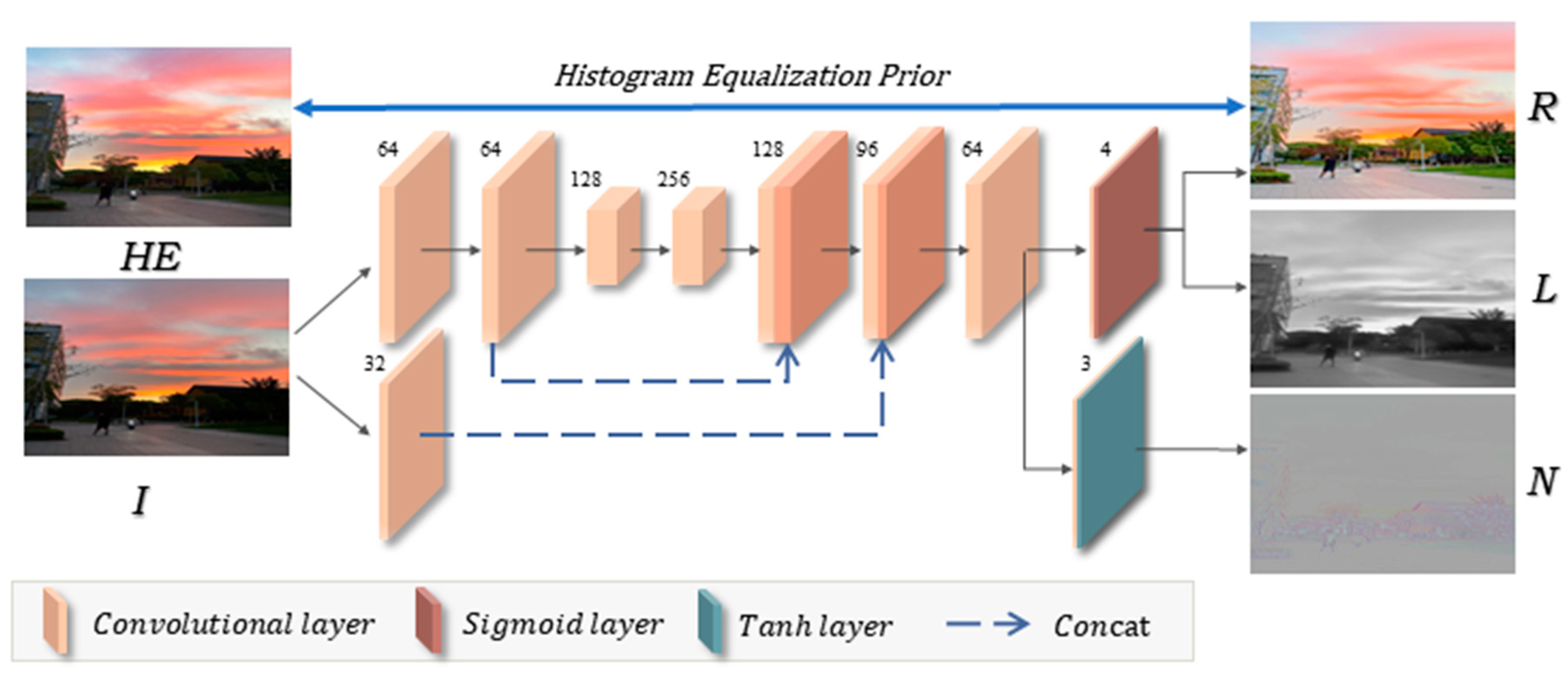
3.1. Enhancement and Denoising Network

The structure of EENet is shown in Figure 2. The robust Retinex model [23] is utilized as an enhancement model for EENet, where image $I$ is decomposed into reflection map $R$, illumination map $L$, and noise map $N$. The details are as follows:

$$I=R\circ L+N$$

(1)

EENet is improved based on the decomposition network [13], which utilizes a simple CNN structure. The sigmoid layer is utilized to decompose $R$ and $L$. Then, an activation layer, a tanh layer [34], is added after the final convolutional layer to simulate additional noise to separate $N$.

Since the feature maps of the histogram equalization-enhanced image are similar to that of ground truth, HEP [15] is introduced to guide the self-supervised network for low-light image enhancement.

We modified the histogram equalization prior perception loss proposed in [15], selected feature maps of different layers in the pre-trained VGG-19 [35] network, and introduced weights, respectively. This allows the feature maps to pay more attention to texture details and improve the visual quality of the enhanced images. This loss function is formulated as follows:

$$L_{hepp}=\sum _l{\lambda }_l{‖{\varphi }_l\left(R\right)-{\varphi }_l\left(H\left(I\right)\right)‖}_1$$

(2)

where $H(·)$ denotes histogram equalization. $l$ represents the layers conv1_1, conv2_1, conv3_1, and conv4_1 of the VGG-19 network. ${\lambda }_l$ and ${\varphi }_l\left(·\right)$ denote the weight and feature map of the $l$-th layer, respectively.

According to Equation (1), the three decomposed maps should be able to be reconstructed into the input image. Therefore, the reconstruction loss is formulated as follows:

$$L_{rec}={‖R\circ L+N-I‖}_1$$

(3)

Since the illumination map $L$ is expected to retain only structural information and ignore details and noise, the illumination loss is defined as follows:

$$L_{is}={‖\left|\mathsf{\nabla }L\right|\circ \exp \left(-{\lambda }_1\ast \left|\mathsf{\nabla }L\right|\right)\circ exp(-{\lambda }_2\ast \left|G\left(\mathsf{\nabla }R\right)\right| \circ \left|\mathsf{\nabla }R\right|)‖}_1$$

(4)

where $\mathsf{\nabla }$ denotes normalized gradient. $G(·)$ represents a smooth filter. ${\lambda }_1$ and ${\lambda }_2$ denote the shape parameters of the loss function.

In the illumination loss, $\left|\mathsf{\nabla }L\right|\ast exp(-\lambda \ast \left|\mathsf{\nabla }L\right|)$ is the smoothness term that separates noise from details, making texture details smoother. $exp(-{\lambda }_2\ast \left|G\left(\mathsf{\nabla }R\right)\right|\circ \left|\mathsf{\nabla }R\right|)$ is the variant of the consistency term [21] that ensures the consistency of the structural information. $\left|G\left(\mathsf{\nabla }R\right)\right|$ denotes the weight term of the image structure; it can smooth the smaller gradients to reduce noise.

To suppress noise amplification in the dark region during enhancement, a noise loss is introduced, which is defined as follows:

$$L_n={‖I\circ N‖}_F$$

(5)

The total loss function of EENet is as follows:

$$L_{EE}=L_{rec}+{\lambda }_{hepp}\ast L_{hepp}+{\lambda }_{is}\ast L_{is}+{\lambda }_n\ast L_n$$

(6)

where ${\lambda }_{hepp}$, ${\lambda }_{is}$, and ${\lambda }_n$ denote the coefficients used to balance the generated reflectance, illumination, and noise map. We empirically set these parameters to ${\lambda }_{hepp}={\lambda }_n=0.01$, and ${\lambda }_{is}=0.1$, respectively.

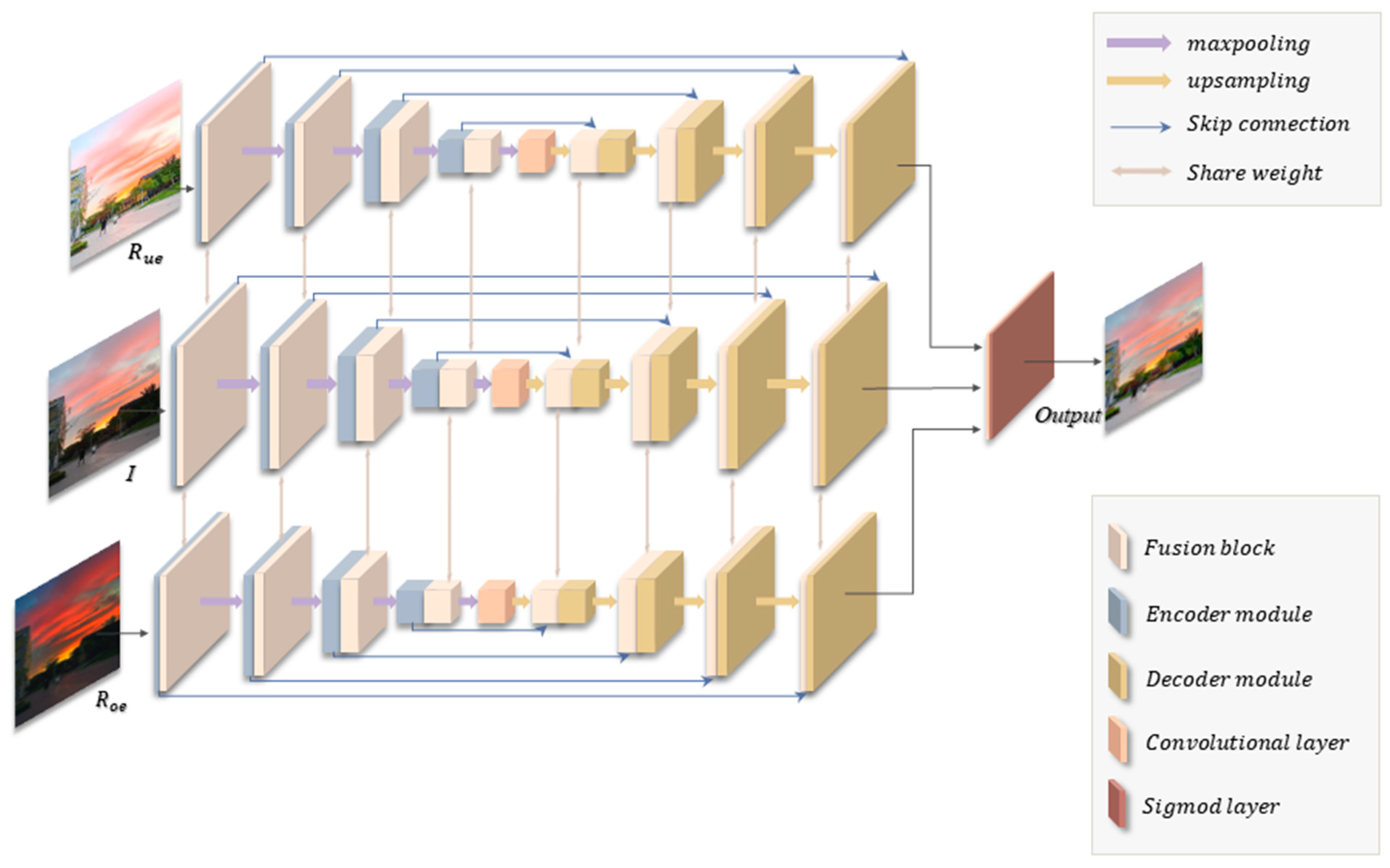
3.2. Three-Branch Asymmetric Exposure Fusion Network

The TAFNet is adopted as our MEF model, as shown in Figure 3. To effectively process each input image, we design the ResUNet, an improvement of the popular U-Net [36] encoder-decoder structure. Then, we introduce the fusion block [37] in ResUNet to enhance feature transfer across branches. Parameter sharing among all branches expedites the fusion process while preserving more details of the resulting fused image. Subsequently, the fused features undergo a sigmoid layer to produce the output image.

Specifically, the ResUNet contains four encoder modules and four decoder modules. Each encoder module consists of two residual blocks [38], while the decoder module consists of three 3 × 3 convolutional layers, as shown in Figure 4. The input and output feature map quantities for encoder and decoder modules are detailed in

Table 1. Input and output feature maps of each encoder and decoder module.

Module	Encoder		Decoder
	m	n	m	n
1	32	64	64	32
2	64	128	128	64
3	128	256	256	128
4	256	512	512	256

. This asymmetric codec network avoids gradient disappearance and preserves more information within the image features. The skip connections are integrated into the ResUNet to reconstruct details at different scales. A 2 × 2 maxpooling operation is applied after each encoder module, and an upsampling layer and feature concatenation operation before each decoder module.

Following each encoding step and preceding the decoding module, the fusion block conducts both maximum and average operations on the features extracted from the three branches. This process enriches feature interactions. Subsequently, these features are concatenated through a 1 × 1 convolutional layer and then individually fed back into each branch.

To guide the self-supervised network for image fusion, the exposure fusion [30] prior is selected as a suitable measure to fuse the bracketed exposure sequence into a well-exposed image.

Specifically, a pixel weight map is calculated for each input image by combining the measures of contrast, saturation, and well-exposedness. It can be denoted as follows:

$$W_{p,k}=\frac{{\left(C_{p,k}\right)}^{{\lambda }_C}\times {\left(S_{p,k}\right)}^{{\lambda }_S}\times {\left(E_{p,k}\right)}^{{\lambda }_E} }{{\sum }_{k=0}^n{\left(C_{p,k}\right)}^{{\lambda }_C}\times {\left(S_{p,k}\right)}^{{\lambda }_S}\times {\left(E_{p,k}\right)}^{{\lambda }_E} }$$

(7)

where $p$, $k$ is the pixel $p$ of the $k$-th image in the image sequence. $C$, $S$, and $E$ represent contrast, saturation, and well-exposedness, respectively. ${\lambda }_C,{\lambda }_S,$ and ${\lambda }_E$ are parameters for controlling each metric. By default, we choose ${\lambda }_C={\lambda }_S={\lambda }_E=1$ [30].

Guided by the pixel weight map, the input three images are weighted for blending to obtain the exposure fusion image, denoted as follows:

$$Q_p=\sum _{k=0}^n{W}_{p,k} \ast I_{p,k}$$

(8)

where $I$ represents the input images, and $Q$ represents the fused image, which will be used as prior information.

The Structural Similarity Index Metric (SSIM) [39] is employed to impose constraints on the similarity between the exposure fusion prior image and the output image, especially in terms of brightness $L$, contrast $C$, and structure $S$. Therefore, the SSIM loss function of TAFNet is defined as follows:

$$L_{SSIM}=+1-SSIM\left(X,F\right)$$

(9)

$$SSIM(X,F)=S(X,F)\times L(X,F)\times C(X,F)$$

(10)

where

$$S\left(X,F\right)=\frac{{\delta }_{XF}+C_1}{{\delta }_X{\delta }_F+C_1}$$

(11)

$$L\left(X,F\right)=\frac{2{\mu }_X{\mu }_F+C_2}{{\mu }_X^2+{\mu }_F^2+C_2}$$

(12)

$$C\left(X,F\right)=\frac{2{\delta }_X{\delta }_F+C_3}{{\delta }_X^2+{\delta }_F^2+C_3}$$

(13)

where ${\mu }_X$, ${\mu }_F$ represent the mean of the output image $X$ and the exposure fusion prior image $F$, respectively. $\delta$ represents the image variance, ${\delta }_{XF}$ represents the covariance of images $X$ and $F$. $C_1$, $C_2$, and $C_3$ are constants.

Adding a perceptual loss [40] enhances the detailed information of the output image features, while avoiding the artifacts generated when the fusion prior image is based on pixel fusion. The perceptual loss is defined as follows:

$$L_{per}=\sum _l{\lambda }_l{‖{\varphi }_l\left(X\right)-{\varphi }_l\left(F\right)‖}_2^2$$

(14)

where ${\varphi }_l\left(·\right)$ still denote the feature map of the VGG-19 network. $l$ are the layers conv1_2, conv2_2, conv3_3, con4_3, and conv5_3.

To make the output image texture clearer, the gradient loss is added to improve the image fusion results, which is defined as follows:

$$L_{grad}=\frac{1}{HW}{‖\mathsf{\nabla }X-\mathsf{\nabla }F‖}_1$$

(15)

where $\mathsf{\nabla }$ represents the gradient. $H$ and $W$ represent the height and width of the image gradient difference, respectively.

The total loss function of TAFNet is as follows:

$$L_{TAF}=L_{SSIM}+{\lambda }_{per}\ast L_{per}+{\lambda }_{grad}\ast L_{grad}$$

(16)

where ${\lambda }_{per}$ and ${\lambda }_{grad}$ denote the coefficients used to enhance the details and textures of the fused images. We empirically set these parameters to ${\lambda }_{per}=0.01$ and ${\lambda }_{grad}=5$, respectively.

4. Experiments and Analysis

4.1. Experimental Settings

We randomly select 1156 images from the ExDark data set [41], which only includes non-uniform low-light images. In total, 1056 of these images are used for training and the rest for validation, and images are resized to 500 × 376. Five publicly available data sets, the DICM [42], LIME [26], MEF [43], NPE [24], and VV [44] data sets, are used for performance evaluation.

We implement the proposed method using the TensorFlow framework on Nvidia RTX 2080Ti GPU. In EENet, batch size and patch size are set to 16 and 48 for training, learning rate and epoch are set to ${10}^{-4}$ and 200. In TAFNet, batch size and patch size are set to 16 and 128 for training, and epoch is set to 60. The initial learning rate is $2.5\times {10}^{-4}$, which is reduced to ${10}^{-4}$ after 25 epochs, and reduced to $5\times {10}^{-5}$ after 40 epochs.

4.2. Main Experiments

Other advanced methods are compared with our proposed method, including supervised methods (RetinexNet [12], KinD [11], MEFGAN [20]), and unsupervised methods (EnlightenGAN [16], Zero-DCE [28], HEP [15], SCI [29], DPE-MEF [21]). Among them, MEFGAN and DPE-MEF are MEF models. The test sets are first enhanced using EENet to obtain $R_{ue}$ and $R_{oe}$, corresponding to the image for underexposure and overexposure, respectively. These images are then fed into the MEF models for further processing.

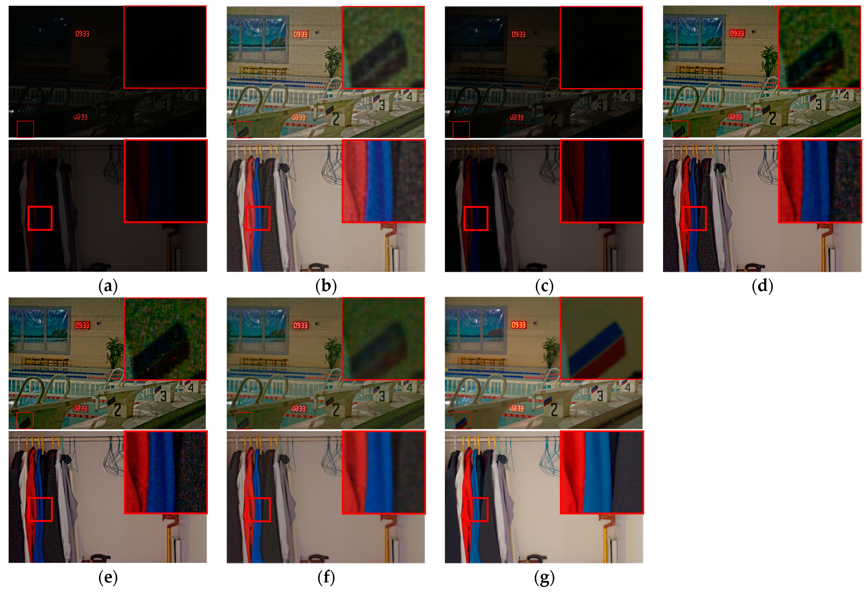
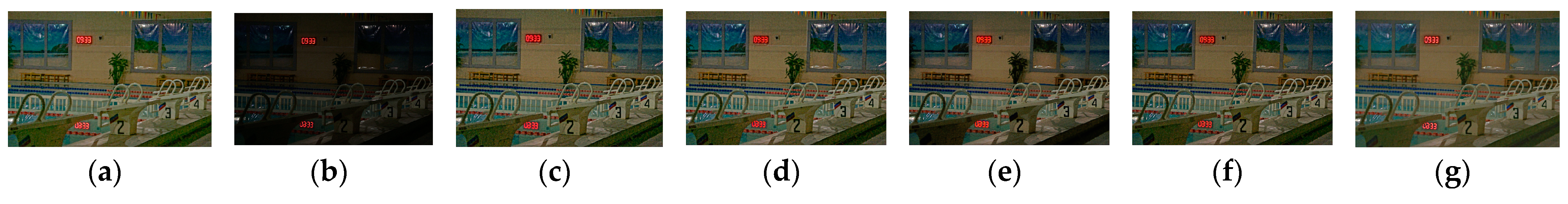
4.2.1. Qualitative Comparison

The visual comparison of enhancement results by the aforementioned methods is presented in Figure 5. The red areas show the image exposure level, while the yellow areas show the noise level. Retinex (corresponding to b in Figure 5) introduces significant color distortion and noise to the enhanced image. KinD(c) and HEP(d) have image denoising. However, they result in varying degrees of image overexposure, as evident in the dolphin in the first column and the clothes in the second column. The same image overexposure exists in SCI, which enhances the image at two different brightness levels, SCI-e(g) and SCI-m(h). EnlightenGAN(f) is a model with an attention mechanism, but still suffers from image overexposure. It also lacks noise suppression, as seen in the sky in the third column. Zero-DCE(e) causes color deviation, such as the window color changing to green in the fourth column. The window color deviations were also observed in the DPE-MEF(j). MEFGAN(i) produces unsatisfactory results. In contrast, EENet(k) can suppress noise amplification and color bias during image enhancement, as observed in the yellow regions of the images in each column. TAFNet in our method(l) corrects the overexposed areas and avoids the loss of details in the output image compared to EENet during the fusion process, as seen in the red region of the images in each column. In summary, our proposed method has superior performance in NLIE processing.

4.2.2. Quantitative Comparison

Quantitative comparisons are analyzed using the zero-reference evaluation metrics Natural Image Quality Evaluator (NIQE) [45] and Blind/Referenceless Image Spatial Quality Evaluator (BRISQUE) [46].

NIQE is the distance between the Multivariate Gaussian (MVG) model for extracting natural scene statistic features from test images and the MVG model for extracting quality perception features from a corpus of natural images, represented as follows:

$$D\left(v_1,v_2,{\Sigma }_1,{\Sigma }_2\right)=\sqrt{\left({\left(v_1-v_2\right)}^T{\left(\frac{{\Sigma }_1+{\Sigma }_2}{2}\right)}^{-1}\left(v_1-v_2\right)\right)}$$

(17)

where $v_1$ and ${\Sigma }_1$ are the mean vector and covariance matrix of the MVG model for natural images, and $v_2$ and ${\Sigma }_2$ are the mean vector and covariance matrix of the MVG model for test images.

BRISQUE fits the mean subtracted contrast normalized (MSCN) coefficients of the test image to an asymmetric generalized Gaussian (AGG) distribution, extracts the features from the fitted Gaussian distribution, and regresses these features as input to a support vector machine to obtain an assessment of image quality. It is defined as follows:

$$f\left(x;v,{\beta }_1,{\beta }_r\right)=\left\{\begin{array}{c}\frac{v}{({\beta }_1+{\beta }_r)\Gamma \left(\frac{1}{v}\right)}exp\left(-{\left(\frac{-x}{{\beta }_1}\right)}^v\right), x<0\\ \frac{v}{({\beta }_1+{\beta }_r)\Gamma \left(\frac{1}{v}\right)}exp\left(-{\left(\frac{x}{{\beta }_r}\right)}^v\right), x\ge 0\end{array}\right.$$

(18)

where $\Gamma \left(\mathrm{x}\right)={\int }_0^{+\infty }{t}^{x-1}{e}^{-t}dt$ is the gamma function; $x>0$ is the shape parameter and ${\beta }_1>0$, ${\beta }_r>0$ are left-scale and right-scale parameters, respectively. AGG density extends generalized Gaussian when ${\beta }_1={\beta }_r$.

Table 2. Quantitative comparisons in terms of NIQE on publicly data sets.

Method	DICM	LIME	MEF	NPE	VV	Mean
RetinexNet	4.51	5.39	4.35	4.40	3.48	4.43
KinD	3.74	4.31	4.31	4.47	3.83	4.13
HEP	3.65	4.28	4.08	5.27	4.78	4.41
EnlightenGAN	2.93	3.88	3.31	3.77	3.19	3.41
Zero-DCE	2.86	4.45	3.43	3.90	3.70	3.66
SCI-e	3.59	4.62	3.88	3.96	3.69	3.95
SCI-m	3.71	4.95	3.70	4.51	4.18	4.21
MEFGAN	5.26	5.15	6.17	5.66	6.41	5.73
DPE-MEF	4.38	5.49	4.62	4.62	3.00	4.42
EENet	3.04	4.10	3.67	3.77	3.01	3.52
Ours	2.84	4.03	3.29	3.81	2.91	3.37

and

Table 3. Quantitative comparisons in terms of BRISQUE on publicly data sets.

Method	DICM	LIME	MEF	NPE	VV	Mean
RetinexNet	31.62	33.94	20.57	21.97	32.42	28.10
KinD	25.09	21.98	35.66	23.78	31.31	27.56
HEP	23.01	24.16	30.60	29.44	40.66	29.57
EnlightenGAN	10.56	30.31	22.83	22.39	28.31	22.88
Zero-DCE	19.99	24.17	22.28	16.56	29.21	22.44
SCI-e	12.31	19.33	19.95	13.51	28.20	18.66
SCI-m	24.89	24.49	18.67	27.24	34.80	26.02
MEFGAN	47.96	36.17	53.11	37.70	56.92	46.37
DPE-MEF	14.11	16.47	17.26	20.02	16.98	16.97
EENet	15.54	19.33	23.63	15.27	14.03	17.56
Ours	11.03	15.87	16.97	17.40	15.25	15.30

show the quantitative results on five publicly available data sets (DICM [42], LIME [26], MEF [43], NPE [24], and VV [44]) using NIQE [45] and BRISQUE [46], respectively. The best result is in bold.

On most of the data sets, EENet in our method has outperformed other methods, and after TAFNet fused and adjusted the images, the evaluation metrics have further improved and achieved the best in average performance metrics, proving the effectiveness of TAFNet.

4.3. Ablation Experiment

4.3.1. Contribution of EENet

Since EENet is a global enhancement model of low-light images, we use the LOL validation set [12], a completely low-light data set, to better verify the ablation experiment. Figure 6 shows the visual results of EENet trained by excluding its loss function one by one. Removing the histogram equalization prior perception loss $L_{hepp}$ fails to enhance the image brightening; removing both the reconstruction loss $L_{rec}$ and the noise loss $L_n$ affects the noise level of the image and cannot improve the quality of the generated image. Removing the illumination loss $L_{is}$ cannot smooth texture details.

Because LOL is a paired data set, the full-reference image assessment metrics Peak Signal to Noise Ratio (PSNR) [47] and SSIM [39] are added to the experiment.

PSNR is an evaluation metric that measures image quality by calculating the mean square error between the test image and the original image. It is defined as follows:

$$PSNR=10\times {\log }_{10}(\frac{{(2^n-1)}^2}{MSE})$$

(19)

$$MSE=\frac{1}{MN}\sum _{i=1}^{M-1}\sum _{j=1}^{N-1}{(X\left(i,j\right)-Y(i,j\left)\right)}^2$$

(20)

where $n$ is the number of image bits, $MSE$ is the Mean Square Error between the test image $X$ and the real image $Y$, and $M$ and $N$ denote the pixel sum of the two images.

SSIM measures the image quality by calculating the structural similarity between the test image and the original image. Its definition can be found in Equations (10)–(13).

Table 4. Results of ablation experiments of EENet on the LOL val set.

Loss Function	PSNR	SSIM	NIQE
w/o ${\mathit{L}}_{\mathit{r}\mathit{e}\mathit{c}}$	20.8190	0.9522	4.7776
w/o ${\mathit{L}}_{\mathit{h}\mathit{e}\mathit{p}\mathit{p}}$	10.8013	0.3289	4.9191
w/o ${\mathit{L}}_{\mathit{i}\mathit{s}}$	21.5714	0.9541	3.8347
w/o ${\mathit{L}}_{\mathit{n}}$	20.0018	0.9586	4.5173
EENet	22.3414	0.9605	3.5511

shows the results of the evaluation of PSNR, SSIM, and NIQE [45] for the LOL validation set. The best result is in bold. The importance of $L_{hepp}$ for model enhancement can be seen, while the other loss functions provide significant improvement in image denoising.

4.3.2. Contribution of TAFNet

To verify the superiority of the structure of TAFNet in the proposed framework, it can better fuse images and remove image artifacts. Figure 7 shows the visual results of TAFNet trained under different network structures. It can be seen that when considering exposure fusion prior (prior), the absence of fusion block (w/o fusion block), and replacing ResUnet with UNet (w/o ResUNet), all these experiments make the image appear with different degrees of artifacts at the fusion boundary.

Table 5. Results of ablation experiments of TAFNet on our val set.

Network STRUCTURE	NIQE	BRIAQUE
prior	2.9547	15.7336
w/o fusion block	2.9496	15.2582
w/o ResUNet	2.9857	15.3832
TAFNet	2.9165	15.2548

shows the results of the evaluation of NIQE and BRISQUE for our validation set, and it can be seen that our constructed TAFNet is more advantageous.

4.4. Effect of Parameters of the Loss Functions

4.4.1. Parametric Analysis of the Loss Function of EENet

In EENet, ${\lambda }_{hepp}$, ${\lambda }_{is}$, and ${\lambda }_n$ represent the weights that guide the generation of the reflection map, illumination map, and noise map, respectively. To analyze the effect of each weight on the model, we set the values at 0.1, 0.01, and 0.001, respectively. For observation and comparison, the validation set and evaluation metrics of the experiments remained the same as the ablation experiments of EENet in Section 4.3.1.

Table 6. Results of the effect of parameters of EENet on the LOL val set.

Parameters	PSNR	SSIM	NIQE
${\lambda }_{hepp}=0.1$, ${\lambda }_{is}=0.1$, ${\lambda }_n=0.01$	22.3946	0.9556	3.5592
${\lambda }_{hepp}=0.001$, ${\lambda }_{is}=0.1$, ${\lambda }_n=0.01$	11.1583	0.3502	4.5630
${\lambda }_{hepp}=0.01$, ${\lambda }_{is}=0.01$, ${\lambda }_n=0.01$	21.7534	0.9757	3.7421
${\lambda }_{hepp}=0.01$, ${\lambda }_{is}=0.001$, ${\lambda }_n=0.01$	21.7233	0.9749	3.5479
${\lambda }_{hepp}=0.01$, ${\lambda }_{is}=0.1$, ${\lambda }_n=0.1$	18.4398	0.9295	4.3532
${\lambda }_{hepp}=0.01$, ${\lambda }_{is}=0.1$, ${\lambda }_n=0.001$	19.7033	0.9512	3.4036
${\lambda }_{hepp}=0.01$, ${\lambda }_{is}=0.1$, ${\lambda }_n=0.01$(EENet)	22.3414	0.9605	3.5511

shows the results of the evaluation of PSNR, SSIM, and NIQE for the LOL validation set. The best result is in bold. Figure 8 shows the visual results of EENet trained by different parameters of the total loss function, with the parameter values corresponding to those of with Table 6.

It can be seen that the brightness of the image decreases when ${\lambda }_{hepp}=0.001$, but when ${\lambda }_{hepp}=0.1$, it obtains the highest PSNR value. The sacrifice of image smoothness resulted in poorer SSIM and NIQE metrics. When ${\lambda }_{is}$ is smaller, the smoothness of the image is worse. When ${\lambda }_n=0.1$, the image sacrifices brightness, and when ${\lambda }_n=0.001$, the image noise is amplified. Taking everything into account, the model performs best when ${\lambda }_{hepp}=0.01$, ${\lambda }_{is}=0.1$, ${\lambda }_n=0.01.$

4.4.2. Parametric Analysis of the Loss Function of TAFNet

In TAFNet, ${\lambda }_{per}$ and ${\lambda }_{grad}$ represent the weights for the perceptual loss and gradient loss, respectively. To analyze the effect of perceptual loss and gradient loss on model content and detail, we set ${\lambda }_{per}$ at 0.001, 0.01, 0.1, and 1, and ${\lambda }_{grad}$ at 1, 5, and 10 for the sensitivity analysis, respectively. For observation and comparison, the validation set and evaluation metrics of the experiments remained the same as the ablation experiments of TAFNet in Section 4.3.2.

Table 7. Results of the effect of parameters of TAFNet on our val set.

Parameters	NIQE	BRISQUE
${\lambda }_{per}=1$, ${\lambda }_{grad}=5$	3.2320	15.2759
${\lambda }_{per}=0.1$, ${\lambda }_{grad}=5$	3.2035	15.9877
${\lambda }_{per}=0.001$, ${\lambda }_{grad}=5$	3.1615	18.7176
${\lambda }_{per}=0.01$, ${\lambda }_{grad}=10$	3.1635	18.4551
${\lambda }_{per}=0.01$, ${\lambda }_{grad}=1$	3.1753	17.7044
${\lambda }_{per}=0.01$, ${\lambda }_{grad}=5$(TAFNet)	2.9165	15.2548

shows the results of the evaluation of NIQE and BRISQUE for our validation set. The best result is in bold. Figure 9 shows the visual results of TAFNet trained by different parameters of the total loss function, with the parameter values corresponding to those of with Table 7.

It can be seen that when the perceptual loss is too large (${\lambda }_{per}=1$) or too small (${\lambda }_{per}=0.001$), the fused image has a color bias, such as the color of sky becomes purple. When the gradient loss is too large (${\lambda }_{grad}=10$) or too small (${\lambda }_{grad}=1$), the texture of the fused image is affected, such as the edges of the white clouds in the figure. Combining the quantitative results, it can be concluded that the image works best when ${\lambda }_{per}=0.01$ and ${\lambda }_{grad}=5$.

4.5. Effect of Data Set

4.5.1. Training on Different Data Sets

To assess the impact of training with different data sets on the model’s robustness, we synthesized a non-uniform low-light image data set by adjusting the brightness and contrast of images sourced from ImageNet [48]. We randomly selected 1098 images for training and 100 images for validation. Since our model is designed for NILE tasks, we did not consider training with entirely low-light image data sets such as the LOL data set.

The testing set included five publicly available data sets (DICM [42], LIME [26], MEF [43], NPE [24], VV [44]), and the DarkFace [49], a nighttime pedestrian detection data set.

Table 8. NIQE indicators of different test sets trained on ImageNet and ExDark data sets.

Data Sets	ExDark	ImageNet	DICM	LIME	MEF	NPE	VV	DarkFace
ImageNet	3.82	4.87	3.15	4.06	3.38	3.75	3.03	2.60
ExDark	3.64	4.82	2.84	4.03	3.29	3.81	2.91	2.59

presents the evaluation using the no-reference quality assessment metric NIQE on different testing sets. Figure 10 partially shows the enhancement results on different test sets, demonstrating that the performance of the model remains stable, whether on synthetic or real image data sets.

4.5.2. Testing in Various Challenging Environments

To evaluate the robustness of the model, we show the enhancement results in various challenging environments, including complex scenes, images with different noise levels, and extreme low-light environments. The test images were chosen from the ExDark data set and real-world images taken by ourselves. We used 10 images in various environmental settings, resulting in a total of 30 test images.

We selected the EnlightenGAN [16], Zero-DCE [28], SCI-e [29], and HEP [15] models for comparison. These methods perform better in image enhancement or denoising compared to the remaining methods.

Table 9. NIQE indicators of different challenging environments.

Methods	HEP	Zero-DCE	EnlightenGAN	SCI-e	Ours
Complex scenes	3.70	3.72	3.69	3.41	2.49
Images with different noise levels	4.51	5.16	4.11	5.47	3.64
Extreme low-light environments	3.36	3.19	3.85	3.92	3.64

shows the evaluation results using the NIQE metric in different environments. The best result is in bold. The enhancement results for different environments are partially shown in Figure 11, where the first, second, and fifth rows are real-world images we took, and the rest belong to the ExDark data set. The first and second rows show complex scenes, the third and fourth rows show images with different noise levels, and the fifth and sixth rows show extreme low-light environments.

It can be seen that the images generated by our method avoid color distortion and contain more details, as observed in the glass in the first row and pedestrians in the second row when compared to other methods in complex environments. In images with different noise levels, our method avoids noise amplification. In particular, compared to HEP(b), which also possesses denoising capabilities, our method sacrifices some brightness in noisier regions but effectively reduces dense noise, as exemplified by the wall in the third row. However, the generated image is less bright in extreme low-light environments. This is due to the operation of suppressing overexposed regions in the proposed method. On the other hand, in extreme low-light environments, there are few overexposed regions, and the brightness of the fused image is sacrificed by the exposure weights during the fusion process.

5. Conclusions

A novel pipeline is proposed to deal with NLIE. By using image inversion and the EENet, we obtain enhanced images that exhibit good exposure in various regions. These enhanced images are subsequently fed into the TAFNet, which effectively solves the problems of uneven exposure and the loss of details in NLIE. Moreover, the whole framework is based on self-supervised learning, which solves the problem of constructing large-scale training data sets. Experimental results show that our proposed method has advantages over existing methods. It is more suitable for complex nighttime image enhancement in the real world. In addition, ablation experiments show that EENet can enhance texture and smooth noise when improving image brightness. TAFNet can effectively fuse images while avoiding image artifacts and color distortion. The appropriate parameter values are determined through experimental sensitivity analysis of the loss function parameters. The stability of the model is demonstrated by training it on different data sets. Furthermore, the robustness of the model is tested under various challenging environments, confirming that the model performs better in complex scenes and images with noise. However, in extreme low-light environments, the enhancement image may compromise some brightness and lose certain details. In the future, our research will focus on achieving a balance between performance and efficiency, and exploring applications in the field of object detection with the aim of significantly improving detection accuracy.

References

1. Zhou, B.; Krähenbühl, P. Cross-view transformers for real-time map-view semantic segmentation. In Proceedings of the IEEE/CVF Conference on Computer Vision and Pattern Recognition, New Orleans, LA, USA, 18–24 June 2022; pp. 13760–13769. [Google Scholar]
2. Wang, C.-Y.; Bochkovskiy, A.; Liao, H.-Y.M. YOLOv7: Trainable bag-of-freebies sets new state-of-the-art for real-time object detectors. In Proceedings of the IEEE/CVF Conference on Computer Vision and Pattern Recognition, Vancouver, Canada, 18–22 June 2023; pp. 7464–7475. [Google Scholar]
3. Yu, F.; Chen, H.; Wang, X.; Xian, W.; Chen, Y.; Liu, F.; Madhavan, V.; Darrell, T. Bdd100k: A diverse driving dataset for heterogeneous multitask learning. In Proceedings of the IEEE/CVF Conference on Computer Vision and Pattern Recognition, Seattle, WA, USA, 16–20 June 2020; pp. 2636–2645. [Google Scholar]
4. Pizer, S.M.; Amburn, E.P.; Austin, J.D.; Cromartie, R.; Geselowitz, A.; Greer, T.; ter Haar Romeny, B.; Zimmerman, J.B.; Zuiderveld, K. Adaptive histogram equalization and its variations. Comput. Vis. Graph. Image Process. 1987, 39, 355–368. [Google Scholar] [CrossRef]
5. Abdullah-Al-Wadud, M.; Kabir, M.H.; Dewan, M.A.A.; Chae, O. A dynamic histogram equalization for image contrast enhancement. IEEE Trans. Consum. Electron. 2007, 53, 593–600. [Google Scholar] [CrossRef]
6. Reza, A.M. Realization of the contrast limited adaptive histogram equalization (CLAHE) for real-time image enhancement. J. VLSI Signal Process. Syst. Signal Image Video Technol. 2004, 38, 35–44. [Google Scholar] [CrossRef]
7. Rahman, Z.-U.; Jobson, D.J.; Woodell, G.A. Retinex processing for automatic image enhancement. J. Electron. Imaging 2004, 13, 100–110. [Google Scholar]
8. Brainard, D.H.; Wandell, B.A. Analysis of the retinex theory of color vision. JOSA A 1986, 3, 1651–1661. [Google Scholar] [CrossRef] [PubMed]
9. Jobson, D.J.; Rahman, Z.-u.; Woodell, G.A. A multiscale retinex for bridging the gap between color images and the human observation of scenes. IEEE Trans. Image Process. 1997, 6, 965–976. [Google Scholar] [CrossRef] [PubMed]
10. Zhang, Y.; Guo, X.; Ma, J.; Liu, W.; Zhang, J. Beyond Brightening Low-light Images. Int. J. Comput. Vis. 2021, 129, 1013–1037. [Google Scholar] [CrossRef]
11. Zhang, Y.; Zhang, J.; Guo, X. Kindling the darkness: A practical low-light image enhancer. In Proceedings of the 27th ACM International Conference on Multimedia, Nice, France, 21–25 October 2019; pp. 1632–1640. [Google Scholar]
12. Wei, C.; Wang, W.; Yang, W.; Liu, J. Deep retinex decomposition for low-light enhancement. arXiv 2018, arXiv:1808.04560. [Google Scholar]
13. Zhang, Y.; Di, X.; Zhang, B.; Wang, C. Self-supervised Image Enhancement Network: Training with Low Light Images Only. arXiv 2020, arXiv:2002.11300. [Google Scholar]
14. Zhang, Y.; Di, X.; Zhang, B.; Li, Q.; Yan, S.; Wang, C. Self-supervised low light image enhancement and denoising. arXiv 2021, arXiv:2103.00832. [Google Scholar]
15. Zhang, F.; Shao, Y.; Sun, Y.; Zhu, K.; Gao, C.; Sang, N. Unsupervised low-light image enhancement via histogram equalization prior. arXiv 2021, arXiv:2112.01766. [Google Scholar]
16. Jiang, Y.; Gong, X.; Liu, D.; Cheng, Y.; Fang, C.; Shen, X.; Yang, J.; Zhou, P.; Wang, Z. EnlightenGAN: Deep Light Enhancement without Paired Supervision. IEEE Trans. Image Process. 2021, 30, 2340–2349. [Google Scholar] [CrossRef] [PubMed]
17. Ni, Z.; Yang, W.; Wang, S.; Ma, L.; Kwong, S. Towards unsupervised deep image enhancement with generative adversarial network. IEEE Trans. Image Process. 2020, 29, 9140–9151. [Google Scholar] [CrossRef] [PubMed]
18. Wang, R.; Jiang, B.; Yang, C.; Li, Q.; Zhang, B. MAGAN: Unsupervised low-light image enhancement guided by mixed-attention. Big Data Min. Anal. 2022, 5, 110–119. [Google Scholar] [CrossRef]
19. Fu, Y.; Hong, Y.; Chen, L.; You, S. LE-GAN: Unsupervised low-light image enhancement network using attention module and identity invariant loss. Knowl. Based Syst. 2022, 240, 108010. [Google Scholar] [CrossRef]
20. Xu, H.; Ma, J.; Zhang, X.-P. MEF-GAN: Multi-exposure image fusion via generative adversarial networks. IEEE Trans. Image Process. 2020, 29, 7203–7216. [Google Scholar] [CrossRef]
21. Han, D.; Li, L.; Guo, X.; Ma, J. Multi-exposure image fusion via deep perceptual enhancement. Inf. Fusion 2022, 79, 248–262. [Google Scholar] [CrossRef]
22. Liu, J.; Wu, G.; Luan, J.; Jiang, Z.; Liu, R.; Fan, X. HoLoCo: Holistic and local contrastive learning network for multi-exposure image fusion. Inf. Fusion 2023, 95, 237–249. [Google Scholar] [CrossRef]
23. Li, M.; Liu, J.; Yang, W.; Sun, X.; Guo, Z. Structure-revealing low-light image enhancement via robust retinex model. IEEE Trans. Image Process. 2018, 27, 2828–2841. [Google Scholar] [CrossRef]
24. Wang, S.; Zheng, J.; Hu, H.-M.; Li, B. Naturalness preserved enhancement algorithm for non-uniform illumination images. IEEE Trans. Image Process. 2013, 22, 3538–3548. [Google Scholar] [CrossRef]
25. Fu, X.; Zeng, D.; Huang, Y.; Liao, Y.; Ding, X.; Paisley, J. A fusion-based enhancing method for weakly illuminated images. Signal Process. 2016, 129, 82–96. [Google Scholar] [CrossRef]
26. Guo, X.; Li, Y.; Ling, H. LIME: Low-light image enhancement via illumination map estimation. IEEE Trans. Image Process. 2016, 26, 982–993. [Google Scholar] [CrossRef]
27. Wu, W.; Weng, J.; Zhang, P.; Wang, X.; Yang, W.; Jiang, J. Uretinex-net: Retinex-based deep unfolding network for low-light image enhancement. In Proceedings of the IEEE/CVF Conference on Computer Vision and Pattern Recognition, New Orleans, LA, USA, 18–24 June 2022; pp. 5901–5910. [Google Scholar]
28. Guo, C.; Li, C.; Guo, J.; Loy, C.C.; Hou, J.; Kwong, S.; Cong, R. Zero-reference deep curve estimation for low-light image enhancement. In Proceedings of the IEEE/CVF Conference on Computer Vision and Pattern Recognition, Seattle, WA, USA, 16–20 June 2020; pp. 1780–1789. [Google Scholar]
29. Ma, L.; Ma, T.; Liu, R.; Fan, X.; Luo, Z. Toward fast, flexible, and robust low-light image enhancement. In Proceedings of the IEEE/CVF Conference on Computer Vision and Pattern Recognition, New Orleans, LA, USA, 18–24 June 2022; pp. 5637–5646. [Google Scholar]
30. Mertens, T.; Kautz, J.; Van Reeth, F. Exposure fusion: A simple and practical alternative to high dynamic range photography. Comput. Graph. Forum 2009, 28, 161–171. [Google Scholar] [CrossRef]
31. Ram Prabhakar, K.; Sai Srikar, V.; Venkatesh Babu, R. Deepfuse: A deep unsupervised approach for exposure fusion with extreme exposure image pairs. In Proceedings of the IEEE International Conference on Computer Vision, Venice, Italy, 22–29 October 2017; pp. 4714–4722. [Google Scholar]
32. Xu, H.; Ma, J.; Le, Z.; Jiang, J.; Guo, X. Fusiondn: A unified densely connected network for image fusion. In Proceedings of the AAAI Conference on Artificial Intelligence, New York, NY, USA, 7–12 February 2020; pp. 12484–12491. [Google Scholar]
33. Xu, H.; Ma, J.; Jiang, J.; Guo, X.; Ling, H. U2Fusion: A unified unsupervised image fusion network. IEEE Trans. Pattern Anal. Mach. Intell. 2020, 44, 502–518. [Google Scholar] [CrossRef] [PubMed]
34. Zhang, L.; Liu, X.; Learned-Miller, E.; Guan, H. SID-NISM: A self-supervised low-light image enhancement framework. arXiv 2020, arXiv:2012.08707. [Google Scholar]
35. Simonyan, K.; Zisserman, A. Very deep convolutional networks for large-scale image recognition. arXiv 2014, arXiv:1409.1556. [Google Scholar]
36. Ronneberger, O.; Fischer, P.; Brox, T. U-net: Convolutional networks for biomedical image segmentation. In Proceedings of the Medical Image Computing and Computer-Assisted Intervention–MICCAI 2015: 18th International Conference, Munich, Germany, 5–9 October 2015; pp. 234–241. [Google Scholar]
37. Zhu, M.; Pan, P.; Chen, W.; Yang, Y. Eemefn: Low-light image enhancement via edge-enhanced multi-exposure fusion network. In Proceedings of the AAAI Conference on Artificial Intelligence, New York, NY, USA, 7–12 February 2020; pp. 13106–13113. [Google Scholar]
38. He, K.; Zhang, X.; Ren, S.; Sun, J. Deep residual learning for image recognition. In Proceedings of the IEEE Conference on Computer Vision and Pattern Recognition, Las Vegas, NV, USA, 27–30 June 2016; pp. 770–778. [Google Scholar]
39. Wang, Z.; Bovik, A.C.; Sheikh, H.R.; Simoncelli, E.P. Image quality assessment: From error visibility to structural similarity. IEEE Trans. Image Process. 2004, 13, 600–612. [Google Scholar] [CrossRef] [PubMed]
40. Johnson, J.; Alahi, A.; Fei-Fei, L. Perceptual losses for real-time style transfer and super-resolution. In Proceedings of the Computer Vision–ECCV 2016: 14th European Conference, Amsterdam, The Netherlands, 11–14 October 2016; pp. 694–711. [Google Scholar]
41. Loh, Y.P.; Chan, C.S. Getting to know low-light images with the exclusively dark dataset. Comput. Vis. Image Underst. 2019, 178, 30–42. [Google Scholar] [CrossRef]
42. Lee, C.; Lee, C.; Kim, C.-S. Contrast enhancement based on layered difference representation. In Proceedings of the 2012 19th IEEE International Conference on Image Processing, Orlando, FL, USA, 30 September–3 October 2012; pp. 965–968. [Google Scholar]
43. Ma, K.; Zeng, K.; Wang, Z. Perceptual quality assessment for multi-exposure image fusion. IEEE Trans. Image Process. 2015, 24, 3345–3356. [Google Scholar] [CrossRef]
44. Vasileios Vonikakis Dataset. Available online: https://sites.google.com/site/vonikakis/datasets (accessed on 16 June 2021).
45. Mittal, A.; Soundararajan, R.; Bovik, A.C. Making a “completely blind” image quality analyzer. IEEE Signal Process. Lett. 2012, 20, 209–212. [Google Scholar] [CrossRef]
46. Mittal, A.; Moorthy, A.K.; Bovik, A.C. No-reference image quality assessment in the spatial domain. IEEE Trans. Image Process. 2012, 21, 4695–4708. [Google Scholar] [CrossRef]
47. Hore, A.; Ziou, D. Image quality metrics: PSNR vs. SSIM. In Proceedings of the 2010 20th International Conference on Pattern Recognition, Istanbul, Turkey, 23–26 August 2010; pp. 2366–2369. [Google Scholar]
48. Deng, J.; Dong, W.; Socher, R.; Li, L.-J.; Li, K.; Fei-Fei, L. Imagenet: A large-scale hierarchical image database. In Proceedings of the 2009 IEEE Conference on Computer Vision and Pattern Recognition, Miami, FL, USA, 20–25 June 2009; pp. 248–255. [Google Scholar]
49. Yuan, Y.; Yang, W.; Ren, W.; Liu, J.; Scheirer, W.J.; Wang, Z. UG2+ Track 2: A Collective Benchmark Effort for Evaluating and Advancing Image Understanding in Poor Visibility Environments. arXiv 2019, arXiv:1904.04474. [Google Scholar]
Figure 1. Pipeline of our NLIE method.
Electronics 12 04445 g001
Figure 2. Overview of our EENet structure.
Electronics 12 04445 g002
Figure 3. Overview of our TAFNet structure.
Electronics 12 04445 g003
Figure 4. Detail of the encoder and decoder module: (a) Encoder module; (b) Decoder module.
Electronics 12 04445 g004
Figure 5. Visual comparison of different methods: (a) input images; (b) RetinexNet [12]; (c) KinD [11]; (d) HEP [15]; (e) Zero-DCE [28]; (f) EnlightenGAN [16]; (g) SCI-e [29]; (h) SCI-m [29]; (i) MEFGAN [20]; (j) DPE-MEF [21]; (k) EENet (our network); and (l) Our method.
Electronics 12 04445 g005aElectronics 12 04445 g005b
Figure 6. Ablation experiments of loss function contribution in EENet. Note that w/o presents results of training without each loss: (a) input; (b) w/o L r e c ; (c) w/o L h e p p ; (d) w/o L i s ; (e) w/o L n ; (f) EENet; (g) ground truth.
Electronics 12 04445 g006
Figure 7. Ablation experiments of network structure contribution of TAFNet on an example of validation data sets: (a) input; (b) prior; (c) w/o fusion block; (d) w/o ResUNet; (e) TAFNet.
Electronics 12 04445 g007
Figure 8. Experiments of the parameters of loss functions in EENet: (a) λ h e p p = 0.1 , λ i s = 0.1 , λ n = 0.01 ; (b) λ h e p p = 0.001 , λ i s = 0.1 , λ n = 0.01 ; (c) λ h e p p = 0.01 , λ i s = 0.01 , λ n = 0.01 ; (d) λ h e p p = 0.01 , λ i s = 0.001 , λ n = 0.01 ; (e) λ h e p p = 0.01 , λ i s = 0.1 , λ n = 0.1 ; (f) λ h e p p = 0.01 , λ i s = 0.1 , λ n = 0.001 ; (g) λ h e p p = 0.01 , λ i s = 0.1 , λ n = 0.01 (EENet).
Electronics 12 04445 g008
Figure 9. Experiments of the parameters of loss functions in TAFNet: (a) λ p e r = 1 , λ g r a d = 5 ; (b) λ p e r = 0.1 , λ g r a d = 5 ; (c) λ p e r = 0.001 , λ g r a d = 5 ; (d) λ p e r = 0.01 , λ g r a d = 10 ; (e) λ p e r = 0.01 , λ g r a d = 1 ; (f) λ p e r = 0.01 , λ g r a d = 5 (TAFNet).
Electronics 12 04445 g009
Figure 10. Visual comparison of image enhancement in different testing sets under ImageNet and ExDark training sets: (a) Input; (b) ImageNet training results; (c) ExDark training results.
Electronics 12 04445 g010
Figure 11. Visual comparison of different methods: (a) input images; (b) HEP [15]; (c) Zero-DCE [28]; (d) EnlightenGAN [16]; (e) SCI-e [29]; and (f) our method. Different challenging environments: complex scenes in the first and second rows; images with different noise levels in the third and fourth rows; and extreme low light environments in the fifth and sixth rows.
Electronics 12 04445 g011