Random Convolutional Kernels for Space-Detector Based Gravitational Wave Signals

Abstract

Neural network models have entered the realm of gravitational wave detection, proving their effectiveness in identifying synthetic gravitational waves. However, these models rely on learned parameters, which necessitates time-consuming computations and expensive hardware resources. To address this challenge, we propose a gravitational wave detection model tailored specifically for binary black hole mergers, inspired by the Random Convolutional Kernel Transform (ROCKET) family of models. We conduct a rigorous analysis by factoring in realistic signal-to-noise ratios in our datasets, demonstrating that conventional techniques lose predictive accuracy when applied to ground-based detector signals. In contrast, for space-based detectors with high signal-to-noise ratios, our method not only detects signals effectively but also enhances inference speed due to its streamlined complexity—a notable achievement. Compared to previous gravitational wave models, we observe a significant acceleration in training time while maintaining acceptable performance metrics for ground-based detector signals and achieving equal or even superior metrics for space-based detector signals. Our experiments on synthetic data yield impressive results, with the model achieving an AUC score of $96.1\%$ and a perfect recall rate of $100\%$ on a dataset with a 1:3 class imbalance for ground-based detectors. For high signal-to-noise ratio signals, we achieve flawless precision and recall of $100\%$ without losing precision on datasets with low-class ratios. Additionally, our approach reduces inference time by a factor of $1.88$.

1. Introduction

Gravitational wave (GW) detection is a prominent area of study in modern physics and has the potential to fundamentally change our understanding of the universe. The first direct observation of GW was made on 14 September 2015 [1,2]. These waves are a result of the dynamics of massive objects like neutron stars and black holes, and they provide a remarkable window into the mysteries of the cosmos [3]. All of the gravitational wave detections made so far, by the Advanced Virgo and Laser Interferometer Gravitational Wave Observatory (aLIGO) detectors, are in accordance with general relativity predictions [4,5,6,7]. Detecting these elusive signals is a complex task that calls for the application of cutting-edge technology as well as meticulous data analysis.

A well-established technique known as matched filtering is used to extract GW signals from instrument data. It convolves templates, i.e., pre-calculated models of the expected signals, with the measured data [8,9]. Nonetheless, due to the significant computational complexity introduced by the large parameter space, matched filtering is far from a real-time process.

Recent developments in machine learning, most notably in neural networks, have improved signal detection performance, making it possible to extract and detect complex signals more quickly and easily [10,11,12,13,14,15]. Eventually, these methods found their application in gravitational wave detection too; some early works utilize convolutional neural networks and achieve competent accuracy and order of magnitude faster inference time when compared to matched filtering [16,17]. The basic premise of these approaches is to train a model with a large number of labeled data using the gradient descent algorithm; this process is referred to as supervised learning.

While neural network-based models have demonstrated strong performance in the detection of gravitational waves, there remains an unexplored opportunity to investigate simpler models. The realm of signal processing has witnessed extensive research that leverages more straightforward concepts, yielding comparable results to those achieved by neural networks [18]. Most cutting-edge models for time series classification typically focus on a single aspect, such as shape, frequency, or variance. In contrast, convolutional kernels offer a unified mechanism capable of capturing a wide range of features without necessitating manual engineering. As an example, a recent study introduces a technique that generates a diverse set of randomly constructed convolutional kernels. When these kernels are combined, they proficiently capture crucial features necessary for time series classification [19,20].

Ground-based gravitational wave detectors have a restricted frequency range for their measurements due to various factors, including seismic noise, thermal noise, quantum noise, and environmental influences. (Martynov et al.) [21] provides an in-depth analysis of the detectors’ sensitivity. The next natural step in GW detection was to broaden the mission to include space-based detectors capable of detecting gravitational waves with frequencies less than 10 Hz. Presently, there are ongoing space-based detector missions, including the Laser Interferometer Space Antenna (LISA), Taiji, and TianQin. LISA, in particular, holds the promise of detecting a wide array of GW sources, encompassing extreme-mass-ratio-inspiral (EMRI), massive black hole binaries (MBHB), and binary white dwarf (BWD) systems [22,23,24]. From a physical standpoint, MBHB events typically yield a very high Signal-to-Noise Ratio (SNR), often exceeding 100. Detecting such signals is straightforward since the noise is negligible. However, for other source types like EMRI and BWD, the SNR tends to hover around 30 [25,26]. To facilitate practical considerations, we focus on gravitational waves falling within the 30–50 SNR range as in [27]. Signals with higher SNRs are virtually guaranteed to be detected, assuming the detection methods are proficient within the lower SNR ranges. The article is structured as follows:

First, we provide an overview of the relevant literature, encompassing a discussion of recent deep learning models applied in GW detection and time series classification methods.

Second, we delve into a detailed description of the ROCKET (Random Convolutional Kernel Transform) family models, alongside an examination of prior time series classification models with similar characteristics. Within this section, we outline the specific modifications and additions we have made to the model.

In the third section, we carry out comparisons with previous time series classification models, culminating in a direct comparison with 1DCNN (One Dimensional Convolutional Neural Network) [17]. It is important to note that we make a clear distinction between classical (quasi-classical) approaches and deep learning models in our comparisons. Our rationale for this approach is twofold: first, we aim to showcase the applicability of the classical model class as a proof of concept before delving into comparisons with the works in this domain.

2. Materials and Methods

2.1. Convolutional Neural Networks (CNN)

CNN are powerful tools for detecting complex patterns. As input moves through the convolution layers, it undergoes a transformative process in which higher complexity characteristics emerge, ready to be used for categorization [28,29,30]. While these networks were initially designed with image classification tasks in mind, necessitating a 2D input structure, they have gracefully transcended their original purpose and found applications in the realm of signal processing. This adaptation to signal processing manifests in two primary forms: the conversion of data into 2D Spectrograms or the employment of 1D convolutions [31].

Within the domain of GW detection, a lively debate ensues regarding the most optimal representation for input signals. Early studies contend that integrating spectrograms with conventional CNN architectures for GW detection yields marginal improvements at best [17]. This contention arises from the inherent challenge of spectrograms, which often forfeit critical information due to the low SNR characteristic of GW signals. In contrast, recent endeavors have embraced a more nuanced approach, leveraging convolutions to extract features from spectrograms in a special manner and even delving into the realm of multi-channel Short-Time Fourier Transform [32,33]. These innovative techniques have yielded commendable performance, reigniting the discourse on signal representation.

A recent innovation in the field brings in a versatile object detection model. Apart from its main job of detecting GW signals, this model also aims to pinpoint the exact location of the signal on a spectrogram by drawing a box around it. This approach represents a significant step forward in the way we detect GW signals [34].

It is also noteworthy to highlight the presence of an open-source GW detection competition [35]. A close examination of the competition’s leaderboards reveals that input signals represented in the one-dimensional strain format tend to yield superior results. Intriguingly, despite the competitive outcomes, the authors have yet to publish formal findings addressing this specific question, leaving it open for future exploration.

2.2. Time Series Classification (TSC) Models

Time series analysis often involves the task of accurately predicting the class of a new time series when we already have time series data labeled with classes. To derive meaningful features from time series data, various methods for time series classification can be employed. Among the earliest and well-known approaches are HIVE-COTE, Shapelet Transform, and BOSS [18].

“Bag-of-SFA Symbols” (BOSS) is a dictionary-based method that extracts words from time series and constructs features representing the frequencies of these words for each time series. BOSS exhibits a quadratic training complexity in both the number of training examples and the length of time series data. While there are more scalable methods like BOSS, they tend to sacrifice accuracy.

The Shapelet Transform Classifier (STF) identifies discriminative subseries in time series data. STF has a training complexity quadratic in the number of training examples and quartic in the length of time series data. Similar to BOSS, there are more scalable alternatives to STF, albeit with lower accuracy.

The Hierarchical Vote Collective of Transformation-based Ensembles (HIVE-COTE) is a heterogeneous meta-ensemble for time series classification. HIVE-COTE assembles classifiers from multiple domains, including BOSS and Shapelet Transform, as well as classifiers based on elastic distance measures and frequency representations. Since its introduction in 2016, HIVE-COTE has been recognized as the most accurate method for time series classification. HIVE-COTE shares a training complexity similar to Shapelet Transform, but its third component, the Elastic Ensemble, involves high computational complexity.

It is evident that all the state-of-the-art methods mentioned above have substantial computational complexity, making them slow even for smaller datasets and entirely impractical for larger datasets. This challenge has driven the development of more scalable methods, such as Inception Time [36], which is an ensemble of deep Convolutional Neural Network models inspired by the Inception-v4 architecture. Inception Time has demonstrated competitiveness with HIVE-COTE.

Although deep learning-based models currently enjoy popularity and preference, it is worth considering simpler methods due to recent advancements in Time Series Classification (TSC) techniques. One such method is ROCKET, which employs convolutional kernels with randomly generated parameters, including length, weight, dilation, and bias. These kernels are applied to the data, and two global features are extracted from the output.

Originally developed for experiments on the UCR archive [37], which contains signals from various domains, ROCKET raises the question of its ability to generalize to noisy signals like GW strain. Various versions of ROCKET have been developed, enabling it to be trained on multi-channel inputs, thereby reducing training time and improving accuracy [20,38,39].

Notably, MiniRocket utilizes critical observations derived from experiments with different hyper-parameter configurations to further reduce the computational complexity of the model.

3. Model

3.1. Rocket and MiniRocket

As a proof of concept, our focus lies on gravitational wave events stemming from binary black hole mergers. However, it is important to emphasize that our model is not confined to this specific context. Furthermore, the versatility of this model becomes evident as it can be readily extended and customized by integrating various classifiers in conjunction with the feature extractor.

Each sample comprises two time series collected simultaneously from two LIGO detectors. Both time series are sampled at 2048 Hz over an 8-second duration. To represent each sample, we stack these two series, resulting in an input shape of $(2,8\times 2048)$. Building upon the methodology outlined in MiniRocket, we employ a set of predefined convolutional kernels to extract features from our input signal.

More formally, we have a set of kernels $K=\{k_1,k_2,k_3\dots k_N\}$, for $k\in K$ and one channel input GW strain x the result of convolution is given by

$$y\left[i\right]=\sum _{j=0}^{l_{\mathrm{kernel}}-1}x[i+(j\times d)]\times k\left[j\right]-b$$

(1)

where d is the dilation, b is the bias and $l_{\mathrm{kernel}}$ is the size of the kernel. We then calculate two ’features’ from $y\left[i\right]$, e.g., $max\left(y\right)$ and $\mathrm{PPV}\left(y\right)=\frac{1}{L}{\sum }_{i=1}^L[y\left[i\right]>0]$ [19]. The process is repeated for each kernel and the features are collected as a row vector. After completing this operation for all the samples we have features of shape $({\mathrm{N}}_{\mathrm{samples}},2·{\mathrm{N}}_{\mathrm{kernels}})$. To accommodate multivariate time series, we perform a summation of the convolution outputs across all the channels. In cases where there are additional detectors, a random subset of channels can be selected. The overall methodology is visualized in Figure 1.

The set of kernels is created based on the following rules, and we will now emphasize the key details below.

• Length—While ROCKET initially employs kernels generated from a set of $\{7,9,11\}$ lengths, it is interesting to note that it observes comparable accuracy when using fixed lengths of 7, 9, and 11, as well as random length selections from $\{9,11,13\}$. Importantly, these differences in accuracy do not reach statistical significance. Based on our experimental findings, we have determined that a fixed kernel size of 9 is an effective choice for our experiment.
• Padding—In the majority of neural networks employing convolutional architectures, a consistent fixed padding is applied across all channels. This practice helps prevent the loss of crucial features at the edges of signals or images during the feature extraction process. Drawing from both standard conventions and insights gleaned from the work of ROCKET, which extensively compared various padding settings, we have arrived at a conclusion: ’zero’ padding proves to be entirely adequate for our purposes.
• Dilation—In the context of ROCKET, various methods of utilizing dilation were analyzed. The findings indicate that employing dilation significantly enhances accuracy, particularly when dilations are sampled from a uniformly distributed exponential scale. This approach effectively enables the capture of both short and long-term patterns in a signal, effectively addressing the issue of the local receptive field.

  $$D=\{\left[2^0\right],\dots ,\left[2^{\max }\right]\}$$

  (2)

  where

  $$\max ={log}_2\left(\frac{l_{\mathrm{input}}-1}{l_{\mathrm{kernel}}-1}\right)$$
• Weights and Bias—Using weights from a fixed set produces similar results to weights initialized randomly, as such and to reduce the computations as proposed in (mini) ROCKET we choose to sample the weights from a set of two values {−1, 2}.
• Biases—Biases are calculated from the outputs of the convolutions. We compute the convolution output for a randomly selected training sample for each kernel/dilation combination and use the quantiles of this output as bias values.

Given the uniqueness of our dataset and the nature of the problem at hand, it becomes essential to recalibrate the number of features. Specifically, because our focus lies on the high-signal-to-noise ratio ($SNR\in [30,50]$) case dataset, we conduct an extensive analysis of different feature map sizes to pinpoint the optimal number of features required, see Figure 2.

Considering the higher SNR, it becomes evident that we require significantly fewer than the default 10,000 features. To determine the ideal number, we conduct a grid search across the range of $[100,1000]$ kernels while working with a low 1/50 dataset ratio. Our findings reveal that after exceeding 1000 features, precision stabilizes at a solid $100\%$. Additionally, since we conducted this analysis with a low signal dataset ratio, it is reasonable to expect that precision will remain consistently high across other ratios as well. Following the feature extraction process, the next step involves selecting a classification model. There is a diverse array of models available for this purpose, providing flexibility in our choice.

For small datasets it is effective to use ridge regression, which applies L2 regularization, this helps with over-fitting issues since we have more features than samples.

$${\widehat{\beta }}^{\mathrm{ridge}}=\underset{\beta }{argmin}\left\{\sum _{i=1}^N{\left(y_i-{\beta }_0-\sum _{j=1}^p{x}_{ij}{\beta }_j\right)}^2+\lambda \sum _{j=1}^p{\beta }_j^2\right\}$$

(3)

Subsequently, we explore various values for regularization parameters and engage in hyperparameter tuning through cross-validation to attain optimal metrics. However, it is worth noting that in our scenario, employing ridge regression is not feasible due to the fact that we have more samples than features.

Our approach involves utilizing logistic regression. Given the typical class imbalance observed in real data and the practical limitation of handling large datasets that cannot be loaded entirely into RAM simultaneously, a more effective strategy is to employ gradient descent with Focal Loss.

Focal Loss introduces an additional factor denoted as ${(1-p_t)}^{\gamma }$ into the standard cross-entropy criterion. The use of Focal Loss [29] enables us to concentrate the training process on the more complex and challenging cases, thereby preventing an overload caused by the sheer volume of straightforward cases that might otherwise burden the detector.

$$\mathrm{FL}\left(p_{\mathrm{t}}\right)=-{\left(1-p_{\mathrm{t}}\right)}^{\gamma }log\left(p_{\mathrm{t}}\right)$$

(4)

where

$$p_{\mathrm{t}}=\left\{\begin{array}{cc}p\hfill & \mathrm{if}y=1\hfill \\ 1-p\hfill & \mathrm{otherwise}\hfill \end{array}\right.$$

(5)

In this scenario, we employ the gradient descent algorithm to train our classifier. This approach enables us to break down the dataset into manageable batches, rather than processing the entire dataset simultaneously.

To optimize our training process, we utilize the ADAM optimizer with parameters: $\beta =(0.9,0.999)$, $ϵ={10}^{-8}$, and weight decay set to 0. We initialize the learning rate at $\mathrm{lr}={10}^{-4}$, which subsequently decreases by a factor of 0.5 (until it reaches ${10}^{-8}$) if the loss does not decrease over 50 mini-batch updates. Our training regimen spans 40 epochs to achieve the desired model performance.

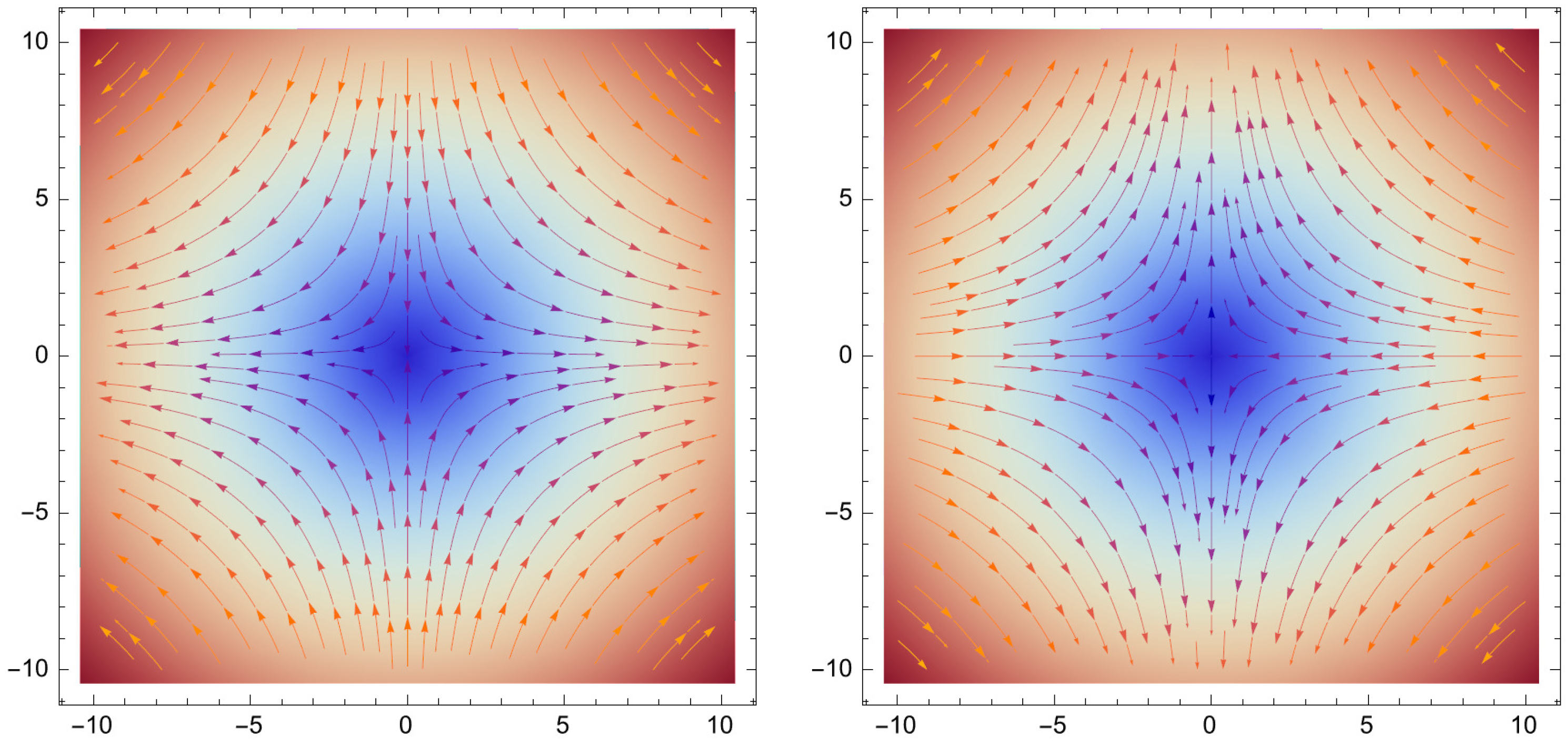
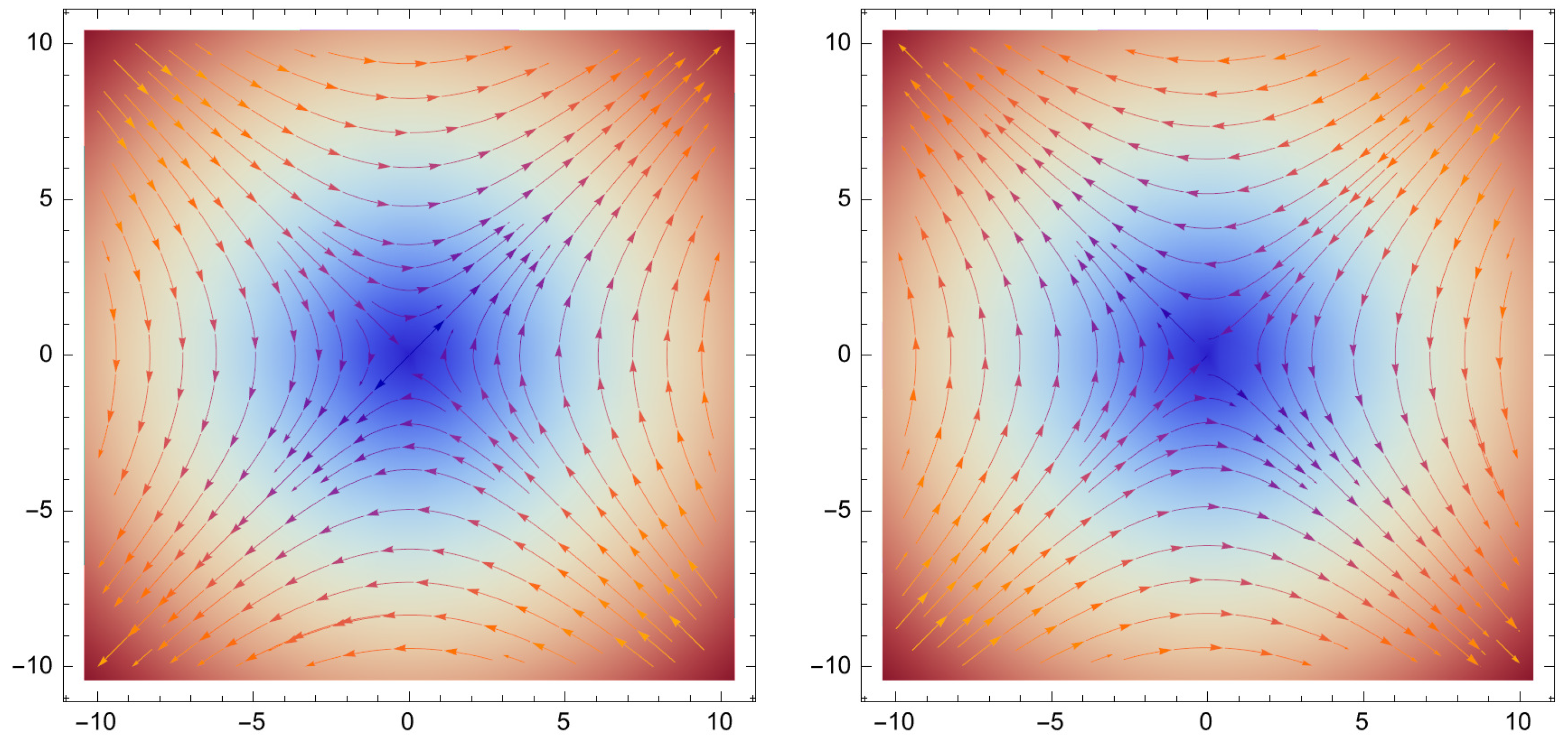
3.2. Feature Map Analysis

As an intriguing side note, we are interested in exploring whether it’s possible to further reduce the feature dimensionality without compromising performance and, ideally, enhancing it. In this section, we introduce a modified method that provides a way to reduce the extensive feature set.

Through this reduction process, we generate a compact set of orthogonal principal components. These components efficiently tackle the problem of overparametrization in the regression classifier. It is important to highlight that while we are focusing on the method for reducing the initial kernel size for MiniRocket here, a similar approach can be extended to ROCKET without compromising its generality.

It is essential to recognize that not all features carry the same weight in the classification process, and some can be safely disregarded. To tackle this challenge, we suggest employing principal component analysis (PCA). This method enables us to extract only a limited number of components that effectively encapsulate a substantial portion of the information contained within the entire dataset.

Principal components offer advantages such as simplifying representation, explaining a significant portion of dataset variance, and addressing overparametrization in regression models.

After completing the feature extraction process, we obtain a matrix $K_{M\times Q}$ where Q represents the number of extracted features. The principal component can then be computed using the following formula:

$$PC=PPV\times W$$

(6)

where W is the weighting matrix constrained by $W^{T}W=1$. The task is to find such values of W that maximize the variances of the corresponding principal component. To find such values, we form the Lagrange function:

$$\begin{array}{cc}\hfill var\left(PPV\right)& =var(PPV\times W)\hfill \\ \hfill var\left(PPV\right)& =W^T\Sigma W\hfill \end{array}$$

where $\Sigma$ is the variance-covariance matrix calculated for the features. Hence the Lagrange function can be represented as follows:

$$L\left(W\right)=W^T\Sigma W-\lambda (W^{T}W-1)$$

(7)

By taking the derivative we obtain the following equation:

$$|\Sigma -\lambda I|W=0$$

(8)

By solving this equation, we can determine the eigenvalues and corresponding eigenvectors. Consequently, the resulting principal components exhibit the following characteristic, denoted as $var\left(P{C}_1\right)\ge var\left(P{C}_2\right)\dots \ge var\left(P{C}_Q\right)$. As a general guideline, it is typically adequate to consider only the initial principal components. In this specific context, utilizing a log-loss function in conjunction with the logistic model is sufficient. We can formulate the log-likelihood function as follows:

$$ln\left(L\right)=\sum _{i=1}^n[y_{i}lnF\left(x_i\beta \right)+(1-y_i)ln(1-F\left(x_i\beta \right))]$$

(9)

where

$$F\left(x\beta \right)=\frac{1}{1+e^{-x\beta }}$$

(10)

Our proposal is to employ the Newton–Raphson optimization algorithm, which typically exhibits rapid convergence to the maximum of the log-likelihood within just a few iterations.

4. Results

4.1. Dataset

Since we will be using an artificially created gravitational wave dataset, it is necessary to be familiar with linearized gravitational wave and detection principle [40]; as such, we will provide a brief summary of these concepts. Gravitational waves are a consequence of Einstein’s General Theory of Relativity. These waves represent propagating ripples in the curvature of space–time itself. From the Einstein Field equation if we consider the linearized case, where the metric tensor can be expressed as

$$g_{\mu \nu }={\eta }_{\mu \nu }+h_{\mu \nu },\left|h_{\mu \nu }\right|\ll 1$$

(11)

where ${\eta }_{\mu \nu }$ is the Minkowski metric and $h_{\mu \nu }$ is a small metric perturbation. Consequently, after simplifications we obtain the familiar wave equation, i.e.,

$$\square {\overline{h}}_{\mu \nu }=0$$

(12)

The general solution to this equation is given in the following form

$${\overline{h}}_{\mu \nu }=\Re \left(A_{\mu \nu }{e}^{i{k}_{\alpha }{x}^{\alpha }}\right)$$

(13)

In a transverse traceless gauge, where most of the components of $A_{\mu \nu }$ tensor are zero, the solution can be simplified to obtain

$${\mathbf{h}}^{TT}=\Re \left[(h_{+}+i{h}_{\times })({\mathbf{e}}^{+}-i{\mathbf{e}}^{\times })\right]$$

(14)

where

$$\begin{array}{cc}\hfill & {\mathbf{e}}^{+}={\overrightarrow{e}}_x\otimes {\overrightarrow{e}}_x-{\overrightarrow{e}}_y\otimes {\overrightarrow{e}}_y\hfill \end{array}$$

(15)

$$\begin{array}{cc}\hfill & {\mathbf{e}}^{\times }={\overrightarrow{e}}_x\otimes {\overrightarrow{e}}_y+{\overrightarrow{e}}_y\otimes {\overrightarrow{e}}_x\hfill \end{array}$$

(16)

are the polarization tensors associated with cross- and plus-polarized waves. Hence, the detectable physical manifestation of a gravitational wave is characterized by a combination of two distinct polarization states, see Figure 3 and Figure 4. The output strain which is registered in the detector is given by the following formula

$$h\left(t\right)=F_{+}(\theta ,\varphi ,\psi )h_{+}\left(t\right)+F_{\times }(\theta ,\varphi ,\psi )h_{\times }\left(t\right)$$

(17)

here $F_{+}$ and $F_{\times }$ are the detector beam patterns and are an integral part of the dataset generation process, the extrinsic parameters are determined after we project the signal into the detectors using these patterns which are given by the following formulas:

$$F_{+}(\theta ,\varphi ,\psi )=\frac{1}{2}(1+{cos}^2\theta )cos2\varphi cos2\psi -cos\theta sin2\varphi sin2\psi$$

(18)

$$F_{\times }(\theta ,\varphi ,\psi )=\frac{1}{2}(1+{cos}^2\theta )cos2\varphi sin2\psi +cos\theta sin2\varphi cos2\psi$$

(19)

Due to the scarcity of real gravitational wave signals, such experiments can currently only be performed on synthetic gravitational wave datasets. The dataset generation process can be accomplished with the help of the Python library “PyCBC” which itself relies on the low-level “LaLSuit” package for the gravitational wave simulations algorithms. It is briefly discussed how the dataset is generated.

• Gravitational wave signals are generated using one of the models provided by the “PyCBC” package, specifically the effective-one-body model designed for spinning, nonprecessing binary black hole mergers, known as SEOBNRV4 [41]. The key input parameters for this model include the masses and spins of the two black holes, which are drawn from Uniform(10, 80) and Uniform(0, 0.998) distributions, respectively. It is worth noting that the SEOBNR family of models has a limitation in that it supports mass ratios only up to 100. Consequently, in cases where one of the celestial bodies possesses significantly more mass than the other, it is advisable to explore alternative numerical models.
• The generated signal is mapped to the detectors using the corresponding antenna patterns, i.e., $F_{+}$ and $F_{\times }$, which are determined by specific values of right ascension, declination, and polarization. These three parameters are randomly sampled from uniform distributions.
• We inject the projected GW signals into additive white Gaussian noise, adjusting their amplitude through rescaling to attain a specific ${\mathrm{SNR}}_{\mathrm{inj}}$, as outlined in the study by Cutler (1994) [42].

  $$s\left(t\right)=h\left(t\right)+n\left(t\right)$$

  (20)

  $$\tilde{h}\left(f\right)={\int }_{-\infty }^{+\infty }h\left(t\right)e^{-2\pi ift}dt$$

  (21)

  $${\left(\frac{S}{N}\right)}_{max}={(h\mid h)}^{1/2}={\left[4\Re \int {\left(\frac{f|\tilde{h}\left(f\right)|}{\sqrt{f{S}_n\left(f\right)}}\right)}^{2}dlnf\right]}^{1/2}$$

  (22)

  $$\rho \equiv \sqrt{\sum _i{\rho }_i^2}$$

  (23)

  where ${\rho }_i$ denotes the SNR for channel i, the final strain can be calculated as follows

  $$s\left(t\right)=\frac{{\mathrm{SNR}}_{\mathrm{inj}}}{\rho }h\left(t\right)+n\left(t\right)$$

  (24)
• The output is then high-passed at 20 Hz to remove some of the simulation’s non-physical turn-on artifacts before being whitened with PYCBC using a local estimate of the power spectral density. The example is then cut to the appropriate length, in this case, 8 seconds, in a way that ensures the signal maximum always falls within the same (relative) region of the sample.

For space-based detector signals with high SNR gravitational wave signals, we follow the recent work of [27]. In their work, they propose gravitational wave data generation for the LISA detector. As a proof of concept, we will only look at the massive black hole mergers model which is conveniently produced by the same SEOBNR model as for black hole mergers.

The key distinctions in the MBHB merger dataset are as follows:

First, the mass values fall within the range of $\mathrm{Uniform}({10}^6,{10}^8)$. Second, the noise component is generated based on a distinct power spectral density, specifically using LISA. Given that the signals produced in this context have a lower frequency range, we can employ a lower sampling rate of 0.1 Hz instead of the typical 2048 Hz for an 8-s signal. This allows us to generate considerably longer signals, extending up to around 160,000 s, all while maintaining the computational efficiency of the arrays. Consequently, we preserve both the signal quality and the required memory resources.

From a technical perspective, the signals detected from such sources only undergo changes in their shape and do not present any additional challenges for detection. The primary distinction lies in the SNR, which makes the detection process significantly easier and more reliable.

4.2. Experimental Section

We have opted for a dataset size of 20,000 samples for training purposes, with an additional 10,000 samples set aside for testing. To begin with, we present the comparison with previous time series classification models.

In terms of classification accuracy, we conducted a comparative analysis of the proposed PC-MiniRocket method against several similar time series classification techniques, including Rocket, MiniRocket, and various other approaches like BOSS, TDE, Shapelet transform, HIVE-COTE 2.0, and Inception Time. To assess the performance of PC-MiniRocket in the context of time series classification, we generated synthetic time series data with different signal-to-noise ratios (SNRs), specifically at levels of 10, 15, 20, 25, and 30. The resulting Figure 5 displayed below illustrates the average ranking of these aforementioned methods.

Based on a two-sided Wilcoxon signed-rank test with Holm correction (utilized as a post hoc test following the Friedman test), algorithms connected by a black line exhibit no statistically significant pairwise differences in their accuracy. Examining Figure 5, we discern that the PC-MiniRocket method outperforms its competitors in terms of classification accuracy. However, it is important to note that the statistical analysis reveals that there is no significant difference in classification accuracy between PC-MiniRocket and MiniRocket, as well as between PC-MiniRocket and HIVE-COTE 2.0. When compared to MiniRocket, there is a slight difference in processing time, which can be attributed to the additional step of principal component extraction in PC-MiniRocket. On the other hand, the faster optimization in PC-MiniRocket can be credited to its use of the Newton method, as opposed to the gradient descent method employed by MiniRocket. This difference in optimization techniques clarifies why, in certain datasets we examined, PC-MiniRocket even outperforms MiniRocket in terms of convergence.

Now, we aim to compare our model with one of the state-of-the-art models in the field of gravitational wave detection, namely the 1DCNN. To enable this comparison, we have introduced a modified version of the 1D-CNN with Focal Loss, and we have generated the dataset with SNR sampled from a Uniform distribution spanning the range of 10 to 20.

To ensure a thorough evaluation of the model’s performance, we have chosen a set of key evaluation metrics, including precision, recall, and F1 score. However, recognizing that selecting a threshold can sometimes lead to misleading conclusions, we have also incorporated the AUC metric into our evaluation. AUC offers a more comprehensive and threshold-agnostic measure of performance, effectively capturing the model’s capabilities without being influenced by specific threshold choices. Additionally, we conduct experiments on different dataset ratios, where $\frac{N_{\mathrm{signal}}}{N_{\mathrm{noise}}}\in$ {3:1, 1:1, 1:3}. The experimental results are shown in

Table 1. Performance analysis of Minirocket for ground-based signal-to-noise ratios (10–20) signals.

S/T	Precision	Recall	AUC	F1
3:1	0.961	1	0.961	0.980
1:1	0.896	1	0.963	0.945
1:3	0.737	1	0.961	0.848

and

Table 2. Performance analysis of 1DCNN for ground-based signal-to-noise ratios (10–20) signals.

S/T	Precision	Recall	AUC	F1
3:1	0.990	0.984	0.998	0.987
1:1	0.958	0.993	0.998	0.975
1:3	0.941	0.980	0.990	0.960

, respectively.

At the outset, we observe that our model’s precision stands at 96%, a value that does not significantly deviate from the precision of the 1DCNN model. However, as we progressively reduce the ratio, an interesting trend emerges. We notice that the precision of our model declines at a notably faster rate compared to the 1DCNN model. In contrast, the AUC score, in this scenario, remains relatively stable. This stable AUC score indicates that our model possesses robust discriminative capabilities, even as the precision experiences a more rapid decline.

To provide a complete and comprehensive perspective, we also include the ROC curve and the Precision-Recall curve, both of which are illustrated in Figure 6.

Additionally, in alignment with prior research, we have calculated and presented the Recall at fixed false positive rates. These values can be readily derived from the ROC curve using piece-wise linear interpolation, as outlined in

Table 3. Recall at fixed false positive rates.

FPR	6%	8.5%	10%
1DCNN	0.993	0.996	0.997
PC-MiniRocket	0.659	0.881	1

.

In summary, the overall performance of our model appears to be slightly less robust compared to the 1DCNN model. However, a noteworthy observation is that our model manages to outperform the 1DCNN model at a 10% False Positive Rate (FPR). Yet, we believe that a more significant insight lies in the consistency of precision/performance across various dataset ratios. To delve deeper into this aspect, we conducted another crucial experiment. In this experiment, we plotted the precision of both models across a dataset ratio range spanning from $\frac{N_{\mathrm{signal}}}{N_{\mathrm{total}}}\in [50\%,0)$. Upon careful analysis of Figure 7, a notable trend emerges. Despite the clear performance margin between the models, it is rather surprising to observe that both models experience a rapid decline in precision as the dataset ratio approaches 0. This phenomenon suggests that neither of the models is well-suited for predicting signals under such conditions. In a real-world scenario, this would likely result in a significant number of false positives. Given that this task revolves around anomaly detection, the expectation is for the model’s performance to remain independent of the dataset composition.

Next, we replicated the same experiment using a high SNR dataset ranging between 30 and 50 for MBHB. In this scenario, we found it adequate to employ MiniRocket with 1000 features, which we recalibrated. It is worth noting that opting for PC-MiniRocket in this context would primarily expedite the training process but would not yield substantial enhancements in terms of model performance. In this case, we can see that the model performance does not drop depending on the dataset ratio and the precision is 100%, see Figure 8.

Additionally, we conducted speed and training time comparisons of the models, and as you can observe, our model has substantially decreased both training and inference times, see

Table 4. Training and inference speed comparison.

Model	Training		Inference
	CPU	GPU	CPU	GPU
1D CNN	N/A	81.25 m	N/A	1.24 ms
PC-MiniRocket	14.4 m	13.5 m	3.64 ms	0.658 ms

.

5. Conclusions

In this study, we have introduced a gravitational wave detection approach based on random convolutional kernels, a recent model in time series classification. We have demonstrated the applicability of this approach to GW signals.

First, we conducted comparisons with previous time series classification methods, revealing that PC-MiniRocket performs on par with MiniRocket for our noisy datasets, showcasing its superior performance.

Secondly, we performed a comparison with one of the state-of-the-art (SOTA) models in the field of GW detection under two scenarios: low SNR ground-based signals and high SNR space-based signals. To ensure a fair evaluation, we employed variable dataset ratios. For low SNR signals, we achieved commendable metrics; however, it became evident that the models’ performance declined as the dataset ratio decreased.

In our subsequent experiment, we observed that both models exhibited exceptional performance, and importantly, they maintained their predictive power even as the dataset ratio decreased.

In conclusion, while 1DCNN displayed better predictive power for low SNR signals, our model demonstrated equivalent performance for high SNR signals while offering the advantages of shorter training and inference times, along with the ability to be implemented on a CPU. These advantages are significant.

In our future work, we plan to explore various methods for effectively handling multichannel input and consider various modifications to enhance its performance for signals with lower SNR.

References

1. Abbott, B.P.; Abbott, R.; Abbott, T.D.; Abernathy, M.R.; Acernese, F.; Ackley, K.; Adams, C.; Adams, T.; Addesso, P.; Adhikari, R.X.; et al. Observation of Gravitational Waves from a Binary Black Hole Merger. Phys. Rev. Lett. 2016, 116, 061102. [Google Scholar] [CrossRef] [PubMed]
2. Abbott, B.P.; Abbott, R.; Abbott, T.D.; Abernathy, M.R.; Acernese, F.; Ackley, K.; Adams, C.; Adams, T.; Addesso, P.; Adhikari, R.X.; et al. Tests of General Relativity with GW150914. Phys. Rev. Lett. 2016, 116, 221101. [Google Scholar] [CrossRef]
3. Branchesi, M. Multi-messenger astronomy: Gravitational waves, neutrinos, photons, and cosmic rays. J. Phys. Conf. Ser. 2016, 718, 022004. [Google Scholar] [CrossRef]
4. Abbott, B.P.; Abbott, R.; Abbott, T.D.; Abernathy, M.R.; Acernese, F.; Ackley, K.; Adams, C.; Adams, T.; Addesso, P.; Adhikari, R.X.; et al. GW151226: Observation of Gravitational Waves from a 22-Solar-Mass Binary Black Hole Coalescence. Phys. Rev. Lett. 2016, 116, 241103. [Google Scholar] [CrossRef]
5. Abbott, B.P.; Abbott, R.; Abbott, T.D.; Abernathy, M.R.; Acernese, F.; Ackley, K.; Adams, C.; Adams, T.; Addesso, P.; Adhikari, R.X.; et al. GW170104: Observation of a 50-Solar-Mass Binary Black Hole Coalescence at Redshift 0.2. Phys. Rev. Lett. 2017, 118, 221101. [Google Scholar] [CrossRef]
6. Abbott, B.P.; Abbott, R.; Abbott, T.D.; Abernathy, M.R.; Acernese, F.; Ackley, K.; Adams, C.; Adams, T.; Addesso, P.; Adhikari, R.X.; et al. GWTC-2: Compact Binary Coalescences Observed by LIGO and Virgo during the First Half of the Third Observing Run. Phys. Rev. X 2021, 11, 021053. [Google Scholar] [CrossRef]
7. Abbott, B.P.; Abbott, R.; Abbott, T.D.; Abernathy, M.R.; Acernese, F.; Ackley, K.; Adams, C.; Adams, T.; Addesso, P.; Adhikari, R.X.; et al. Observation of Gravitational Waves from Two Neutron Star–Black Hole Coalescences. Astrophys. J. Lett. 2021, 915, L5. [Google Scholar] [CrossRef]
8. Turin, G. An introduction to matched filters. IRE Trans. Inf. Theory 1960, 6, 311–329. [Google Scholar] [CrossRef]
9. Owen, B.J.; Sathyaprakash, B.S. Matched filtering of gravitational waves from inspiraling compact binaries: Computational cost and template placement. Phys. Rev. D 1999, 60, 022002. [Google Scholar] [CrossRef]
10. Purwins, H.; Li, B.; Virtanen, T.; Schlüter, J.; Chang, S.Y.; Sainath, T. Deep Learning for Audio Signal Processing. IEEE J. Sel. Top. Signal Process. 2019, 13, 206–219. [Google Scholar] [CrossRef]
11. Li, X.; Ban, Y.; Girin, L.; Alameda-Pineda, X.; Horaud, R. Online Localization and Tracking of Multiple Moving Speakers in Reverberant Environments. IEEE J. Sel. Top. Signal Process. 2019, 13, 88–103. [Google Scholar] [CrossRef]
12. Famoriji, O.J.; Shongwe, T. Deep Learning Approach to Source Localization of Electromagnetic Waves in the Presence of Various Sources and Noise. Symmetry 2023, 15, 1534. [Google Scholar] [CrossRef]
13. Famoriji, O.J.; Ogundepo, O.Y.; Qi, X. An Intelligent Deep Learning-Based Direction-of-Arrival Estimation Scheme Using Spherical Antenna Array with Unknown Mutual Coupling. IEEE Access 2020, 8, 179259–179271. [Google Scholar] [CrossRef]
14. Famoriji, O.J.; Shongwe, T. Multi-Source DoA Estimation of EM Waves Impinging Spherical Antenna Array with Unknown Mutual Coupling Using Relative Signal Pressure Based Multiple Signal Classification Approach. IEEE Access 2022, 10, 103793–103805. [Google Scholar] [CrossRef]
15. Li, X.; Girin, L.; Horaud, R.; Gannot, S. Multiple-Speaker Localization Based on Direct-Path Features and Likelihood Maximization With Spatial Sparsity Regularization. IEEE/ACM Trans. Audio Speech Lang. Process. 2017, 25, 1997–2012. [Google Scholar] [CrossRef]
16. Gebhard, T.D.; Kilbertus, N.; Harry, I.; Schölkopf, B. Convolutional neural networks: A magic bullet for gravitational-wave detection? Phys. Rev. D 2019, 100, 063015. [Google Scholar] [CrossRef]
17. George, D.; Huerta, E.A. Deep neural networks to enable real-time multimessenger astrophysics. Phys. Rev. D 2018, 97, 044039. [Google Scholar] [CrossRef]
18. Bagnall, A.; Lines, J.; Bostrom, A.; Large, J.; Keogh, E. The Great Time Series Classification Bake Off: A Review and experimental evaluation of recent algorithmic advances. Data Min. Knowl. Discov. 2016, 31, 606–660. [Google Scholar] [CrossRef] [PubMed]
19. Dempster, A.; Petitjean, F.; Webb, G.I. ROCKET: Exceptionally fast and accurate time series classification using random convolutional kernels. Data Min. Knowl. Discov. 2020, 34, 1454–1495. [Google Scholar] [CrossRef]
20. Dempster, A.; Schmidt, D.F.; Webb, G.I. MiniRocket: A Very Fast (Almost) Deterministic Transform for Time Series Classification. In Proceedings of the KDD’21 27th ACM SIGKDD Conference on Knowledge Discovery & Data Mining; Association for Computing Machinery: New York, NY, USA, 2021; pp. 248–257. [Google Scholar] [CrossRef]
21. Martynov, D.; Hall, E.D.; Abbott, B.P.; Abbott, R.; Abbott, T.D.; Adams, C.; Adhikari, R.X.; Anderson, R.A.; Anderson, S.B.; Arai, K.; et al. Sensitivity of the Advanced LIGO detectors at the beginning of gravitational wave astronomy. Phys. Rev. D 2016, 93, 112004. [Google Scholar] [CrossRef]
22. Amaro-Seoane, P.; Audley, H.; Babak, S.; Baker, J.; Barausse, E.; Bender, P.; Berti, E.; Binetruy, P.; Born, M.; Bortoluzzi, D.; et al. Laser Interferometer Space Antenna. arXiv 2017, arXiv:1702.00786. [Google Scholar]
23. Hu, W.R.; Wu, Y.L. The Taiji Program in Space for gravitational wave physics and the nature of gravity. Natl. Sci. Rev. 2017, 4, 685–686. [Google Scholar] [CrossRef]
24. Luo, J.; Chen, L.S.; Duan, H.Z.; Gong, Y.G.; Hu, S.; Ji, J.; Liu, Q.; Mei, J.; Milyukov, V.; Sazhin, M.; et al. TianQin: A space-borne gravitational wave detector. Class. Quantum Gravity 2016, 33, 035010. [Google Scholar] [CrossRef]
25. Gair, J.; Hewitson, M.; Petiteau, A.; Mueller, G. Space-Based Gravitational Wave Observatories. In Handbook of Gravitational Wave Astronomy; Bambi, C., Katsanevas, S., Kokkotas, K.D., Eds.; Springer: Singapore, 2020; pp. 1–71. [Google Scholar] [CrossRef]
26. Kupfer, T.; Korol, V.; Shah, S.; Nelemans, G.; Marsh, T.R.; Ramsay, G.; Groot, P.G.; Steeghs, D.T.H.; Rossi, E.M. LISA verification binaries with updated distances from Gaia Data Release 2. Mon. Not. R. Astron. Soc. 2018, 480, 302–309. [Google Scholar] [CrossRef]
27. Zhao, T.; Lyu, R.; Wang, H.; Cao, Z.; Ren, Z. Space-based gravitational wave signal detection and extraction with deep neural network. Commun. Phys. 2023, 6. [Google Scholar] [CrossRef]
28. He, K.; Zhang, X.; Ren, S.; Sun, J. Deep Residual Learning for Image Recognition. arXiv 2015, arXiv:1512.03385. [Google Scholar]
29. Lin, T.Y.; Goyal, P.; Girshick, R.; He, K.; Dollár, P. Focal Loss for Dense Object Detection. arXiv 2018, arXiv:1708.02002. [Google Scholar]
30. Simonyan, K.; Zisserman, A. Very Deep Convolutional Networks for Large-Scale Image Recognition. arXiv 2015, arXiv:1409.1556. [Google Scholar]
31. Kiranyaz, S.; Ince, T.; Abdeljaber, O.; Avci, O.; Gabbouj, M. 1-D Convolutional Neural Networks for Signal Processing Applications. In Proceedings of the ICASSP 2019—2019 IEEE International Conference on Acoustics, Speech and Signal Processing (ICASSP), Brighton, UK, 12–17 May 2019; pp. 8360–8364. [Google Scholar] [CrossRef]
32. Fan, S.; Wang, Y.; Luo, Y.; Schmitt, A.; Yu, S. Improving Gravitational Wave Detection with 2D Convolutional Neural Networks. In Proceedings of the 2020 25th International Conference on Pattern Recognition (ICPR), Milan, Italy, 10–15 January 2021; pp. 7103–7110. [Google Scholar] [CrossRef]
33. Jiang, L.; Luo, Y. Convolutional Transformer for Fast and Accurate Gravitational Wave Detection. In Proceedings of the 2022 26th International Conference on Pattern Recognition (ICPR), Montreal, QC, Canada, 21–25 August 2022; pp. 46–53. [Google Scholar] [CrossRef]
34. Aveiro, J.; Freitas, F.F.; Ferreira, M.; Onofre, A.; Providência, C.; Gonçalves, G.; Font, J.A. Identification of binary neutron star mergers in gravitational-wave data using object-detection machine learning models. Phys. Rev. D 2022, 106, 084059. [Google Scholar] [CrossRef]
35. Chris, M.; Christopher, Z.; Elena, C.; Michael, J.W.; Walter, R. G2Net Gravitational Wave Detection. 2021. Available online: https://kaggle.com/competitions/g2net-gravitational-wave-detection (accessed on 17 October 2023).
36. Fawaz, H.I.; Lucas, B.; Forestier, G.; Pelletier, C.; Schmidt, D.F.; Weber, J.; Webb, G.I.; Idoumghar, L.; Muller, P.-A.; Petitjean, F. InceptionTime: Finding AlexNet for time series classification. Data Min. Knowl. Discov. 2020, 34, 1936–1962. [Google Scholar] [CrossRef]
37. Dau, H.A.; Bagnall, A.; Kamgar, K.; Yeh, C.C.M.; Zhu, Y.; Gharghabi, S.; Ratanamahatana, C.A.; Keogh, E. The UCR Time Series Archive. arXiv 2019, arXiv:1810.07758. [Google Scholar] [CrossRef]
38. Tan, C.W.; Dempster, A.; Bergmeir, C.; Webb, G.I. MultiRocket: Multiple pooling operators and transformations for fast and effective time series classification. arXiv 2022, arXiv:2102.00457. [Google Scholar] [CrossRef]
39. Salehinejad, H.; Wang, Y.; Yu, Y.; Jin, T.; Valaee, S. S-Rocket: Selective Random Convolution Kernels for Time Series Classification. arXiv 2022, arXiv:2203.03445. [Google Scholar]
40. Thorne, K.S.; Blandford, R.D. Modern Classical Physics; Princeton University Press: Princeton, NJ, USA, 2017. [Google Scholar]
41. Bohé, A.; Shao, L.; Taracchini, A.; Buonanno, A.; Babak, S.; Harry, I.W.; Hinder, I.; Ossokine, S.; Pürrer, M.; Raymond, V.; et al. Improved effective-one-body model of spinning, nonprecessing binary black holes for the era of gravitational-wave astrophysics with advanced detectors. Phys. Rev. D 2017, 95, 044028. [Google Scholar] [CrossRef]
42. Cutler, C.; Flanagan, E.E. Gravitational waves from merging compact binaries: How accurately can one extract the binary’s parameters from the inspiral waveform? Phys. Rev. D 1994, 49, 2658–2697. [Google Scholar] [CrossRef] [PubMed]
Figure 1. Scheme of the model with multi-channel input (convolutional outputs are not on the same scale for visualization purposes).
Electronics 12 04360 g001
Figure 2. Precision depending on the features extracted for high-range signal-to-noise ratios signals (30–50).
Electronics 12 04360 g002
Figure 3. Field lines representing the tidal acceleration field of the plus-polarized wave that produces the cloud’s deformation, at a phase when h ¨ + > 0 (left) and h ¨ + < 0 (right).
Electronics 12 04360 g003
Figure 4. Field lines representing the tidal acceleration field of the cross-polarized wave that produces the cloud’s deformation, at a phase when h ¨ × > 0 (left) and h ¨ × < 0 (right).
Electronics 12 04360 g004
Figure 5. Mean rank of PC-MiniRocket against other algorithms.
Electronics 12 04360 g005
Figure 6. ROC, Precision-Recall curves for 1:3 classes, 10–20 signal-to-noise ratios.
Electronics 12 04360 g006
Figure 7. Precision over data balance ranging from [ 50 % , 0 % ) for 10–20 signal-to-noise ratios.
Electronics 12 04360 g007
Figure 8. Precision over data balance ranging from [ 5 % , 2 % ] for 30–50 signal-to-noise ratios.
Electronics 12 04360 g008