The Markov Concept of the Energy Efficiency Assessment of the Edge Computing Infrastructure Peripheral Server Functioning over Time

Abstract

The article is devoted to the research of the peripheral server energy consumption managing process defined based on the threshold policy by manipulating the values of the characteristic parameters of the arithmetic-logical complex of the latter. The research object is formalized by a Markov queue model with a single-threshold control scheme for the intensity of accepted requests service. A characteristic feature of the life cycle of a peripheral server is the non-stationary mode of operation in terms of energy consumption, due to the need to periodically poll the controlled sensor network and process the received data in real-time. To take into account this circumstance, the intensities of transitions in the heterogeneous birth-and-death Markov process of the created model are interpreted as non-random periodic functions of time. The resulting mathematical apparatus is summarized in the metric that allows us to estimate the target peripheral server’s energy consumption both at a specific moment and for a censored time interval (this distinguishes the obtained result from existing analogs).

1. Introduction

1.1. Research Background

When developing a network infrastructure, one usually considers either local computing or cloud computing. But these two options and their combinations are not enough. For example, what to do if you cannot refuse cloud computing, but there is not enough bandwidth or the traffic is too expensive? Add an intermediate link that will perform part of the calculations at the edge of the local network or production process. This modern edge concept is called Edge Computing [1,2,3,4,5] and harmonizes the current cloud data usage model.

As peripheral nodes in Edge Computing, the corresponding servers [6,7,8,9] are used, which are placed directly where information is produced. Usually, these are production or technical premises in which it is impossible to mount a server rack and ensure cleanliness. Considering such extreme placement conditions, peripheral server cases are made, first of all, protected from moisture and dust. At the same time, significantly less attention is paid to the organization of their cooling. Taking into account the last fact, the energy efficiency of the operation of such devices determines not only their efficiency but also their service life. Considering that the topology of sensor networks in which such peripheral servers are involved is constantly growing, the relevance of ensuring the energy efficiency of the latter is becoming an increasingly urgent task.

In the context of our study, the mechanisms for achieving the energy efficiency of computing elements are of greater interest. We will mention the most popular ones [1,2,3], namely the on-off method, the dynamic frequency scaling method (also known as CPU throttling), and the dynamic voltage scaling method. These methods reflect two real ways to reduce processor power consumption:

−

turn off some subsystems;

−

reduce frequency or voltage.

Operations aimed at implementing each of the mentioned ways to reduce power consumption are summarized in the corresponding instruction sets: C-states, and P-states.

C-states describe the first way to reduce processor power consumption, which is why they are called idle states. To disable a subsystem, nothing should be running on it. Thus, the C[X] C-state means that one or more processor subsystems, referred to as X, are disabled. P-states describe the second case. Processor subsystems are running but do not require maximum performance, so the clock speed and/or voltage for that subsystem may be reduced. Thus, P[X] P-state means that the computing subsystem operates at a set frequency, which corresponds to the ordinal number of state X (more on this below).

Let us mention the main C-states (defined in the Advanced Configuration and Power Interface (ACPI) standard [10] with subject comments:

−

C0: Active, the processor/core is executing instructions. The P-states are used here, the processor/core can work in maximum performance mode (P0) or power saving mode (in a state other than P0);

−

C1: Halt, the processor does not execute instructions, but can instantly return to the C0 state. Because the processor is idle, the P-states are not relevant for states different than C0.

P-states imply that the processor is in the C0 state because it needs the power to execute instructions. P-states allow us to change the frequency and voltage of the cores (in other words, the operating mode) to reduce power consumption. There is a set of P-states, each corresponding to other operating modes (frequency-voltage pairs). Most often, the choice of the P-state is implemented through the operating system. We can select the operating frequency (by specifying the appropriate P-state code), and the voltage is selected by the computational unit depending on the selected frequency and another factor. After the P-state is requested by writing to the unit-dependent register, the voltage is changed to the firmware-calculated value and the clock oscillator switches to a specified frequency. All computational unit cores share the same P-state. The P-state change is instantaneous, so a lot of transitions can be made per second. This is in contrast to C-state transitions, which take longer and require energy spending.

Having outlined a modern approach to managing processor power consumption using the policy of determining C- and P-states, we can make some generalizations in the context of the fact that our server is a peripheral computing element of an Edge Computing infrastructure. Such a peripheral server, on the one hand, periodically polls the sensor network it manages to collect data. On the other hand, it processes the collected data in real-time and sends the report to the cloud. Such a schedule of operation is remarkably implemented in the energy consumption policy $\mathrm{C}3\mathrm{P}0$ (maximum performance in the active phase—maximum energy saving (hibernation) in the rest of the time). The problem is that at any time a request for an extraordinary data collection can be received from the cloud or instructions can be received to correct the schedule, and the peripheral server must respond as quickly as possible. Thus, the acceptable base C-state for the peripheral server is C0. If we talk about P-states, then in the active phase this is, of course, P0. In the waiting phase, this will be the P-state with the number N (the last number provided for the current processor model). Such a $\mathrm{C}0\mathrm{P}0|\mathrm{C}0\mathrm{PN}$ scheme is known to researchers as a $T$ policy which we will discuss in more detail below.

1.2. Related Works

Several concepts and related technologies have already been developed for server power management. It should be noted that each of them has its advantages and disadvantages. We will not make a detailed review of specialized technologies—this has already been performed by respected colleagues [11,12,13,14,15]. But let us, however, pay closer attention to two works. In the survey [16], the authors focus on an interesting class of terminal edge devices that operate in the mode of power consumption from batteries for most of their life cycle. The authors of [16] postulate that all processing and interpretation of data in such devices is performed in the cloud, which reduces the load on the computing platform and reduces the rate of battery discharge but determines significantly higher requirements for the quality of communications. At the same time, the authors of the mentioned survey single out the issue of energy efficiency of peripheral servers as especially important. As an obvious justification for the relevance of such researchers, the authors mention that about 33% of all energy dissipation in the world falls on cyber-physical systems involved in the manufacturing industry. In such systems, both the edge computing paradigm and the corresponding infrastructure, including peripheral servers, are actively used. Even if the latter accounts for a tenth of a percent of the total amount of dissipated energy, this is still a colossal value, even a slight decrease which will have a huge economic and environmental effect.

Investigating the phenomenon of energy consumption of computing elements and their complexes, scientists often resort to modeling the paradigm of queuing systems with different control schemes. In such a case, the researcher’s task is to find an appropriate control scheme for the components of the simulated computing device or their associated composition by analyzing the corresponding characteristics of the queuing system under certain initial conditions. Among the numerous scientific and applied works on this topic, it is worth noting the works [17,18,19,20,21,22] (systems with $D$ policy), [19,23,24,25] (systems with $N$ policy), [24,25,26,27,28] (systems with $T$ policy). Despite the sufficient development of the subject area, research in this direction is constantly relevant. This is facilitated by the constant evolution of technological platforms on which modern computing, information and communication conglomerates are built.

We focus on describing the power consumption of a peripheral server based on a queuing system with a threshold policy. In this case, it is necessary to pay attention to the key parameters that characterize the efficiency of queuing systems that describe the functioning of computing subsystems. Among these parameters, we mention [29,30,31] the intensity of the outgoing flow of requests, the probability of servicing, the probability of losing requests, the average waiting time for requests in the queue, the average time the request stays in the system, the average queue length, the average number of busy service channels, the average number of requests in the system. The focus is on the properties of monotony and convexity (concavity) of these characteristics. This emphasis is due to the desire of researchers to determine simple approximating expressions for combinations of functional dependencies of these characteristics within given boundaries. At the moment, these dependencies are defined for many types of queuing systems [10,11,12,13,14,15,16], which does not negate the obvious fact that these parameters are not directly related to the power consumption characteristics of computing systems as such. As a result, it is difficult for engineers to interpret such mathematical models to evaluate the energy efficiency of real computing systems. A simple and unambiguously interpretable metric is needed, the formalization of which to describe the energy consumption of computing operations on a peripheral server is the focus of this article.

However, it will not be too categorical and we will unambiguously determine the closest analog for the research problem mentioned in the article. Article [27] is devoted to the issue of increasing the energy efficiency of the basic computing element of the Data Center, i.e., the server, due to the implementation of the mechanism of threshold control of the processor clock frequency. The authors of this article used a $T$ policy $M|M|1$ queuing system as the server model. According to this policy, if the total number of requests accepted by the model (to be processed target data packets) is less than $T$, then the intensity of their service is equal $f_0$. When the total number of accepted requests is greater than or equal to $T$, then the intensity of their service instantly becomes equal $f>f_0$. The $T$ policy considered by the authors coincides with the usual threshold service intensity management strategy, which has been repeatedly described in the literature on queuing systems. Without focusing on the mathematical results obtained by the authors of [27] concerning the properties (monotonicity, convexity) of the main stationary characteristics of the model depending on the value of $T$, we focus our attention on the practical value of the mentioned article. It consists in formalizing the transition from the mathematical model to the energy efficiency characteristics of the server. Also, the mentioned article presents the results of computational experiments (the dependence of the average power consumption in the stationary mode on the corresponding controlled parameters). All the results presented in [27] were obtained under the assumption that both the intensity of request receipt and the intensity of their service do not depend on time. This limitation is easily explained by the fact that the Data Center server operates in a mode close to stationary. It is this circumstance that does not allow us to describe the life cycle of a peripheral server in terms of the mathematical apparatus described in the mentioned article. Despite this, the study of the issues raised in the mentioned article regarding the investigation of the energy efficiency of a peripheral server is of undoubted interest. In this case, we will need to take into account that in the model we create, the intensities will be non-random functions of time. It is this mode of operation that is typical for a peripheral server, the life cycle of which can be characterized by an inhomogeneous birth-and-death Markov process.

1.3. Research Attributes

Next, the authors identified the main attributes of scientific research.

The object of research is the energy consumption managing process of the Edge Computing infrastructure peripheral server over time, defined based on the threshold policy.

The subject of research includes the theory of probability and mathematical statistics, the theory of Markov processes, and the queuing theory.

The purpose of the research is formulated as follows: to analytically formalize in simple energy efficiency metrics the process of functioning of the Edge Computing infrastructure peripheral server, represented by the $M\left(t\right)|M\left(t\right)|1|\infty$ Markov queuing system with $T$ policy, in time.

Accordingly, the objectives of the research are:

−

analytically formalize the Markov concept of the energy efficiency assessment of the Edge Computing infrastructure peripheral server functioning over time,

−

analytically formalize the approach for determining time-uniform estimates of the approximation error of the original multiparameter weakly ergodic Markov process using processes with a lower number of states,

−

analytically determine the main probabilistic characteristics of the research object based on the proposed concept using the above-mentioned approach,

−

justify the adequacy of the proposed mathematical apparatus and demonstrate its functionality in the context of the research purpose.

Let us formulate the main contribution of the research. The material of the article is devoted to the research of the peripheral server energy consumption managing process defined based on the threshold policy by manipulating the values of the characteristic parameters of the arithmetic-logical complex of the latter. This process is formalized by a Markov queue model with a single-threshold control scheme for the intensity of accepted requests service. A characteristic feature of the life cycle of a peripheral server is the non-stationary mode of operation in terms of energy consumption, due to the need to periodically poll the controlled sensor network and process the received data in real-time. To take into account this circumstance, the intensities of transitions in the heterogeneous birth-and-death Markov process of the created model are interpreted as non-random periodic functions of time. The resulting mathematical apparatus is summarized in the metric that allows us to estimate the target peripheral server’s energy consumption both at a specific moment and for a censored time interval.

2. Materials and Methods

2.1. Statement of the Research

Edge Computing is a viable solution for organizations whose activities involve processing data in real-time. This distributed computing paradigm focuses on data processing, storage, and analytics at the edge of the network (closer to the data source). This approach can provide numerous benefits, including improved performance, increased security, and reduced latency. At the same time, computing resources at the edge of the network are limited compared to the power of central cloud servers. This circumstance actualizes the problem of ensuring the energy efficiency of computing on the peripheral server as a basic unit in the Edge Computing infrastructure.

As a model of the peripheral server, we will use the Markov queuing system, in which we will predict the dependence of transitions on time, that is, $M\left(t\right)|M\left(t\right)|1|\infty$. As a basic scheme for managing the energy efficiency of peripheral server calculations, we will use the $T$ policy in the author’s interpretation, where the number $T\ge 2$, $T\in \mathbb{N}$, will be called the threshold. As long as the number of requests in the model is less than $T$, the system serves them with an exponential intensity with a characteristic of ${\eta }_0\left(t\right)$. When the moment $t\ge 0$ comes, when the number of requests is accepted by the model $\ge T$, the law of their service by the system changes $\eta \left(t\right)$, $\eta \left(t\right)>{\eta }_0\left(t\right)$. At the same time, we will assume that the accepted requests will be served by the system in the order of arrival, and the switching of the model between non-random functions $\left\{{\eta }_0\left(t\right),\eta \left(t\right)\right\}$ takes place instantly.

The dynamics of changes in the peripheral server’s energy availability over time are characterized by a non-homogeneous Markov chain $\left\{S\left(t\right),t\ge 0\right\}$ with continuous time and a family of discrete states $S=\left\{i\right\}$, $i\ge 0$, $i\in \mathbb{N}$. The state index $i\in S$ represents the number of requests accepted by the model. The logic of the system’s functioning assumes that the model can transit from the state $i$ only to neighboring states: $\left\{i-1,i+1\right\}$.

We characterize the Markov process $S\left(t\right)$ with transition probabilities $p_{ij}\left(x,t\right)=\mathrm{Pr}\left\{S\left(t\right)=j|S\left(x\right)=i\right\}$, $0\le x\le t$. The probability that at moment $t$ process $S\left(t\right)$ is in state $i$ is characterized by the value $p_i\left(t\right)=\mathrm{Pr}\left(S\left(t\right)=i\right)$, $i\ge 0$. Let us summarize these probabilistic characteristics in the form of a vector $\overrightarrow{p}\left(t\right)={\left\{p_i\left(t\right)\right\}}^{\mathrm{T}}$, $i\ge 0$.

Let us introduce the concept of a small time interval $\tau \ge 0$. Taking this parameter into account, we redefine the transition probabilities of the process $S\left(t\right)$ as

$$\mathrm{Pr}\left(S\left(t+\tau \right)=j|S\left(t\right)=i\right)=\{\begin{array}{l}\mu \left(t\right)\tau +{\lambda }_{ij}\left(t,\tau \right)\forall j=i++,i\ge 0;\\ {\eta }_0\left(t\right)\tau +{\lambda }_{ij}\left(t,\tau \right)\forall j=i--,i=\overline{1,T--};\\ \eta \left(t\right)\tau +{\lambda }_{ij}\left(t,\tau \right)\forall j=i--,i\ge T;\\ {\lambda }_{ij}\left(t,\tau \right)\forall \mathrm{other}\hspace{0.17em}\hspace{0.17em}\mathrm{cases},\end{array}$$

(1)

where ${\sup }_i\left|{\lambda }_{ij}\left(t,\tau \right)\right|=o\left(\tau \right)$, and $\mu \left(t\right)$ is a characteristic of the Poisson intensity of the arrival of new requests to the model.

Taking this into account, we determine the transition intensities matrix of the process $S\left(t\right)$ in the form of a three-diagonal matrix:

$$Q\left(t\right)=\left(\begin{array}{cccccccccc}-\mu \left(t\right)& \mu \left(t\right)& 0& 0& \dots & 0& 0& 0& 0& \dots \\ {\eta }_0\left(t\right)& -{\nu }_0\left(t\right)& \mu \left(t\right)& 0& \ddots & 0& 0& 0& 0& \dots \\ 0& {\eta }_0\left(t\right)& -{\nu }_0\left(t\right)& \mu \left(t\right)& \ddots & 0& 0& 0& 0& \dots \\ ⋮& \ddots & \ddots & \ddots & \ddots & \ddots & \ddots & \ddots & \ddots & ⋮\\ 0& 0& 0& 0& \ddots & {\eta }_0\left(t\right)& -{\nu }_0\left(t\right)& \mu \left(t\right)& 0& \dots \\ 0& 0& 0& 0& \ddots & 0& \eta \left(t\right)& -{\nu }_0\left(t\right)& \mu \left(t\right)& \dots \\ 0& 0& 0& 0& \ddots & 0& 0& \eta \left(t\right)& \mu \left(t\right)& \dots \\ ⋮& ⋮& ⋮& ⋮& ⋮& ⋮& ⋮& ⋮& ⋮& \ddots \end{array}\right),$$

where ${\nu }_0\left(t\right)=\mu \left(t\right)+{\eta }_0\left(t\right)$, $\nu \left(t\right)=\mu \left(t\right)+\eta \left(t\right)$.

Let us generalize the matrix $Q\left(t\right)$ and probabilities $p_i\left(t\right)$ in the form of a system of Chapman’s differential equations:

$$\frac{d\overrightarrow{p}\left(t\right)}{dt}=Q^{\mathrm{T}}\left(t\right)\overrightarrow{p}\left(t\right).$$

(2)

Note, that the time-inhomogeneous Markov chain $S\left(t\right)$ is weakly ergodic if, for any initial conditions ${\overrightarrow{p}}^{\ast }\left(t\right)$, ${\overrightarrow{p}}^{\ast \ast }\left(t\right)$, the $\Vert {\overrightarrow{p}}^{\ast }\left(t\right)-{\overrightarrow{p}}^{\ast \ast }\left(t\right)\Vert \to 0$ holds at $t\to \infty$, where ${\overrightarrow{p}}^{\ast }\left(t\right)$, ${\overrightarrow{p}}^{\ast \ast }\left(t\right)$ are the corresponding solutions of the system of Equations (2), and $\Vert \dots \Vert$ is the $l_1$ norm.

Let us define the mathematical expectation of the process $S\left(t\right)$ (the average number of accepted requests) as $M_k\left(t\right)=M\left\{S\left(t\right)|S\left(0\right)=k\right\}$ with initial conditions $S\left(0\right)={\overrightarrow{m}}_k$. Starting from this definition, we say that the function $\varphi \left(t\right)$ is the limiting mean for $S\left(t\right)$ if the equality $\underset{t\to \infty }{\lim }\left(\varphi \left(t\right)-M_k\left(t\right)\right)=0$ is fulfilled $\forall k$.

Further analytical constructions are formulated taking into account the following reasonable assumptions:

−

the intensities of receiving and servicing requests are periodic with the same period $h$ (the polling of the sensor array placed on the data source is carried out with the specified periodicity),

−

the service intensity of received requests by the system is proportional: ${\eta }_0\left(t\right)=k\eta \left(t\right)$, $0<k<1$ (this reproduces the possibility of manipulating the FID multiplier provided in the Intel SpeedStep and AMD Cool’n’Quiet firmware).

2.2. The Markov Concept of the Edge Computing Infrastructure Peripheral Server Functioning over Time

Let us denote the average intensities of receiving and servicing requests by the system $\overline{\eta }=\frac{1}{h}{\displaystyle \underset{0}{\overset{h}{\int }}\eta }\left(t\right)dt$, ${\overline{\eta }}_0=\frac{1}{h}{\displaystyle \underset{0}{\overset{h}{\int }}{\eta }_0}\left(t\right)dt$, $\overline{\mu }=\frac{1}{h}{\displaystyle \underset{0}{\overset{h}{\int }}\mu }\left(t\right)dt$. Then, using the theorem presented in Appendix A, generalized by expressions (A2), (A3), and its corollary (A5) (the reason for including these materials in the appendix is that, according to the authors, these materials will be of greater interest to theoretical mathematicians, while the main text of the article has an applied orientation), we can formulate several statements that are directly relevant to our research.

We can classify a process $S\left(t\right)$ as weakly ergodic if the inequality $\overline{\mu }<\overline{\eta }$ holds. Under such conditions, $t\to \infty$ for any initiating values ${\overrightarrow{p}}^{\ast }\left(0\right)$, ${\overrightarrow{p}}^{\ast \ast }\left(0\right)$, such estimates of the convergence rate as

$$\Vert {\overrightarrow{p}}^{\ast }\left(t\right)-{\overrightarrow{p}}^{\ast \ast }\left(t\right)\Vert \le 4L{e}^{-\overline{\nu }t}{\displaystyle \sum _{i\ge 1}{z}_i\left|p_i^{\ast }\left(0\right)-p_i^{\ast \ast }\left(0\right)\right|},$$

(3)

will be admissible, where $L=e^{{\displaystyle \underset{0}{\overset{h}{\int }}{\eta }_0\left(t\right)dt}}$, $\overline{\nu }=\left(\sqrt{{\overline{\eta }}_0}-\sqrt{\overline{\mu }}\right)$, $z_i={\displaystyle \sum _{n=1}^i{b}_n}$, $b_n={\alpha }^{n-1}$, $\alpha =\sqrt{{\overline{\eta }}_0/\overline{\mu }}$. At $\forall k$:

$$\left|M_k-\varphi \left(t\right)\right|\le 4\frac{L}{V}{e}^{-\overline{\nu }t}{\Vert \overrightarrow{p}\left(0\right)-{\overrightarrow{e}}_k\Vert }_{iB},$$

(4)

where $V=\underset{n\ge 1}{\inf }\frac{{\alpha }^{n-1}}{n}$, $1B\in l_1$.

If we develop the theorem presented in Appendix A in the direction of estimating the solution error of the Chapman system of the form (2) for a process $S\left(t\right)$ with a set of states $\mathrm{S}=\left\{i\right\}$, $i=\overline{0,N}$, and intensities $\overline{\eta }$, ${\overline{\eta }}_0$, $\overline{\mu }$, then for the resulting $\overrightarrow{p}\left(t\right)$, ${\overrightarrow{p}}_N\left(t\right)$ probabilities the inequality

$$\Vert \overrightarrow{p}\left(t\right)-{\overrightarrow{p}}_N\left(t\right)\Vert \le 8\frac{L^{3/2}}{{\overline{\nu }}^{3/2}{\alpha }^{N-1}}{C}_{\mu }\left(C_{\mu }+C_{\eta }\right),$$

(5)

will hold at $\overrightarrow{p}\left(0\right)={\overrightarrow{e}}_0$, ${\overrightarrow{p}}_N\left(0\right)=\overrightarrow{p}\left(0\right)$ where the constants $C_{\mu }$, $C_{\eta }$ limit at $t\in \left[0,\infty \right)$ the linear combinations of the finite number of locally integrated functions of the intensities $\mu \left(t\right)$ and ${\eta }_0\left(t\right)$, $\eta \left(t\right)$, respectively: $\mu \left(t\right)\le C_{\mu }<\infty$, ${\eta }_0\left(t\right),\eta \left(t\right)\le C_{\eta }<\infty$.

By analogy with expression (5), for the limit values of the process $S\left(t\right)$ mathematical expectation, the following estimate will be true:

$$\left|M_0\left(t\right)-M_{0,N}\left(t\right)\right|\le 4\frac{L^{3/2}}{V{\overline{\nu }}^{3/2}{\alpha }^{N-1}}{C}_{\mu }\left(C_{\mu }+C_{\eta }\right).$$

(6)

2.3. The Metric for the Energy Efficiency Assessment of the Studied Process

Let us connect the obtained in Section 2.2 probabilistic-time characteristics with the established interpretation of the concept of energy efficiency of computing elements. The well-known formula [27] for energy consumption (used power) of a computer system $\mathsf{\Pi }$:

$$\mathsf{\Pi }=C{U}^{2}f+{\mathsf{\Pi }}_s,$$

(7)

where $C$ is the capacity of transistor gates, $f$ is the frequency of the algorithmic-logic conglomerate (central processor only or a central processor and graphics subsystem), $U$ is the supply voltage, and ${\mathsf{\Pi }}_s$ is the constant power consumption incl. energy consumption for the functioning of communication equipment located in the peripheral server.

The values of the parameters $C$, $U$, ${\mathsf{\Pi }}_s$ will be constant for a particular peripheral server. The speed of data processing changes synchronously with the change in the clock frequency $f$ of the algorithmic-logical conglomerate as part of the peripheral server. Suppose that if the number of requests for data processing in the buffer of the algorithmic-logical conglomerate is less than $T$, then the latter functions with a clock frequency of $f_0$. If the number of accepted data processing requests in the queue is equal to or exceeds $T$, then the clock frequency is equal to $f>f_0$. As a result, the consumed power $\mathsf{\Pi }$ transcendentally depends on the threshold $T$ due to the current value of the clock frequency $f$.

For the general case, we will assume that the dependence of the service intensity of received requests ${\eta }_0\left(t\right)$, $\eta \left(t\right)$ on the clock frequency of the algorithmic-logic complex s has a linear character:

$${\eta }_0\left(t\right)=C_{\beta }{f}_0\beta \left(t\right), \eta \left(t\right)=C_{\beta }f\beta \left(t\right),$$

(8)

where $\beta \left(t\right)$ is a non-random periodic function of time, the existence of which is based on the periodicity of polling of the sensor network by the peripheral server, and the coefficient $C_{\beta }$ is a constant of the computing potential, the value of which is determined as a result of an independent external evaluation of the algorithmic-logical complex of the peripheral server using, for example, constantly updating the AIDA64 utility (versions 6.*). This software product of FinalWire Ltd. (Budapest, Hungary) is justifiably popular due to the availability of objective tests of the components of personal computers running the MS Windows operating system.

We integrate the mathematical apparatus formalized in the section, which characterizes the process of functioning of the peripheral server, represented by the Markov queue system $M\left(t\right)|M\left(t\right)|1|\infty$ defined within the framework of $T$ policy, in time, into expression (7) taking into account functional dependencies (8):

$$\mathsf{\Pi }\left(t,T,f,f_0\right)=C{U}^2\left[f\left(1-{\displaystyle \sum _{i=0}^{T-1}{p}_i\left(t\right)}\right)+f_0\left(1-{\displaystyle \sum _{i=0}^{T-1}{p}_i\left(t\right)}\right)\right]+{\mathsf{\Pi }}_s,$$

(9)

Since characteristic (9) depends on time, it is expedient to investigate the averaged version of this characteristic, i.e., $\overline{\mathsf{\Pi }}\left(t,T,f,f_0\right)$. Let us define a sufficiently long time interval $\left[t,t+\overline{t}\right]$, in which $\overline{t}$ is the interval during which all functional and service operations performed periodically by the peripheral server are fully manifested. Under such circumstances, we formalize the characteristic $\overline{\mathsf{\Pi }}\left(t,T,f,f_0\right)$ with the expression

$$\overline{\mathsf{\Pi }}\left(t,T,f,f_0\right)=\frac{1}{\overline{t}}{\displaystyle \underset{0}{\overset{\overline{t}}{\int }}\mathsf{\Pi }}\left(t,T,f,f_0\right)dt.$$

(10)

Expression (10) can be interpreted as the average energy consumption (used power) of the peripheral server during time $\left[t,t+\overline{t}\right]$.

3. Results

In this section, we will focus on simulating the computing process of a peripheral server whose computing subsystem changes the rate of information packet service by the $T$-policy. At the same time, we will present the simulation results in metrics (9) and (10), focused on the representation of the studied process in the context of energy consumption.

In Section 2, we presented the computational process of a peripheral server as a $M\left(t\right)|M\left(t\right)|1|\infty$ queuing system, in which the client is an information package, and the processor pipeline is a device. The first dependence $M\left(t\right)$ in the abbreviation of the created queuing system means that packets arrive at the input of the queuing system by Poisson’s law and intensity $\mu$, i.e., the time between arrivals of packets is characterized by an exponential law with the same steamer. The second dependence $M\left(t\right)$ in the abbreviation of the created system characterizes the service of received packets. Accordingly, the time to service the information packet is also characterized by an exponential law. At the same time, the implementation of the threshold policy predetermines that the service time is distributed exponentially with two different parameters ${\eta }_0$ and $\eta$. The logic of the created system provides that switching from low service intensity ${\eta }_0$ to high service intensity $\eta$ occurs automatically if the number of received information packets exceeds the threshold value $T$. Note, that the packet arrival time and service time are independent parameters. Finally, the number 1 in the abbreviation of the created system means that one processor unit is involved in servicing packets. In general, the system $M\left(t\right)|M\left(t\right)|1|\infty$ implements a first-in-first-out discipline for servicing received information packets (without priorities). Thus, the created model fully reflects the specifics of the studied process.

We will demonstrate the functionality of the mathematical apparatus presented in Section 2 in practice with an orientation to the popular Dell PowerEdge XE family. This choice determines the values of some parameters-constants mentioned in expression (7) fundamental for the target metric (9), (10). Based on the Dell PowerEdge XE family specification, let us define $U=1.35$ V, ${\mathsf{\Pi }}_s=5$ W, $f_0,f\in \left[2.4,2.7\right]$ GHz, $C\approx 14.23$ nF (for $U=1.35$ V, ${\mathsf{\Pi }}_s=5$ W, $f=2.7$ GHz).

We will determine the function of the intensities of the arrival of new requests to the model $\mu \left(t\right)$ and the function $\beta \left(t\right)$, which regulates the periodicity of this process:

$$\mu \left(t\right)=0.8+0.01\sin \left(2\pi t\right), \beta \left(t\right)=1+0.033\sin \left(0.04\pi t\right).$$

(11)

Note, that the need to take into account periodic dependencies (11) reflects the specifics of the operation of the peripheral server, in which the sensor network is polled as a rule with some periodicity.

To preserve the comparability of the author’s results with the closest analog [27], we define the constant $C_{\beta }$ as $0.37$.

The set values and functions allow us to determine the intensity of processing requests by the system according to expression (8) as ${\eta }_0\left(t\right)=0.37\left(1+0.033\sin \left(0.04\pi t\right)\right)f_0$, $\eta \left(t\right)=0.37\left(1+0.033\sin \left(0.04\pi t\right)\right)f$.

Finally, we will form a plan for experiments. We have already mentioned that we summarize the mathematical apparatus pressed down in Section 2 in the form of useful metric (9), (10) that allows us to estimate the target peripheral server’s energy consumption $\mathsf{\Pi }$ both at a specific moment (expression (9)) and for a censored time interval (expression (10)). The main characteristic parameters of the metric are the threshold $T$ (the capacity of the accepted for processing data packets queue), the base frequency $f_0$ (before the threshold is exceeded) and the operating frequency $f$ of the computing subsystem (after the threshold is exceeded), and time $t$. Thus, in general terms, the power consumption of a peripheral server in the proposed metric is a function of four parameters, which does not allow us to present the results of experiments in one figure. Next, we will show how the metric (9) and (10) reacts to a change in each of the four characteristic parameters for fixed values of the corresponding three of them.

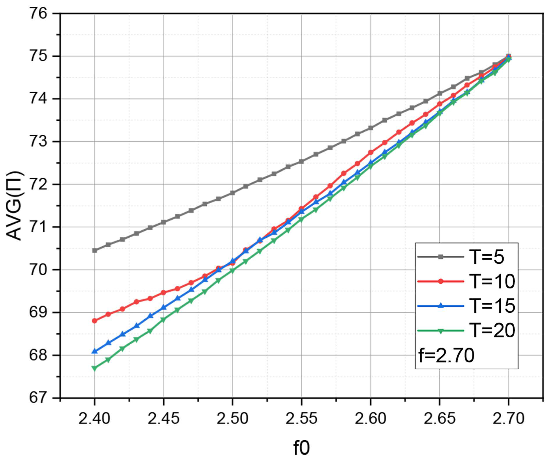
Based on the defined parameters and functions, we calculate the value of the variant of the characteristic (10) for $f_0\in \left[2.40,2.70\right]$, $f=2.70$ and $T=\left\{5,10,15,20\right\}$. The calculation results are visualized in Figure 1 and

Table 1. The exact values of the dependencies are presented in Figure 1.

${\mathit{f}}_0$	$\overline{\mathbf{\Pi }}$ $\mathbf{at} \mathit{T}=5$	$\overline{\mathbf{\Pi }}$ $\mathbf{at} \mathit{T}=10$	$\overline{\mathbf{\Pi }}$ $\mathbf{at} \mathit{T}=15$	$\overline{\mathbf{\Pi }}$ $\mathbf{at} \mathit{T}=20$
2.40	70.45036	68.80499	68.08606	67.70365
2.41	70.58829	68.95846	68.28542	67.90301
2.42	70.71095	69.08133	68.48477	68.16355
2.43	70.84887	69.25011	68.68417	68.3782
2.44	70.98678	69.3271	68.9141	68.57758
2.45	71.10941	69.46529	69.11347	68.83817
2.46	71.24733	69.55757	69.32809	69.06805
2.47	71.38524	69.69575	69.52749	69.28274
2.48	71.53842	69.84921	69.75744	69.4974
2.49	71.66106	70.03327	69.98739	69.75794
2.50	71.79898	70.15615	70.20206	69.98791
2.51	71.95214	70.4626	70.43201	70.20256
2.52	72.10533	70.67727	70.69258	70.44784
2.53	72.24326	70.95309	70.86131	70.69307
2.54	72.41172	71.15247	71.10658	70.93832
2.55	72.53434	71.42831	71.35184	71.18358
2.56	72.70282	71.70418	71.58183	71.41353
2.57	72.85601	71.96471	71.78112	71.67408
2.58	73.00919	72.25586	72.04171	71.91932
2.59	73.17763	72.48583	72.27166	72.1646
2.60	73.31552	72.74634	72.50159	72.42515
2.61	73.49925	72.9763	72.74687	72.6551
2.62	73.65244	73.22155	72.97681	72.91564
2.63	73.79033	73.43624	73.20678	73.16089
2.64	73.94351	73.63558	73.452	73.37554
2.65	74.12724	73.88086	73.69729	73.66669
2.66	74.28041	74.0802	73.95783	73.92724
2.67	74.47939	74.32546	74.15719	74.14189
2.68	74.61731	74.52482	74.43304	74.41775
2.69	74.80102	74.73947	74.66299	74.61709
2.70	74.99998	74.96944	74.95415	74.92352

.

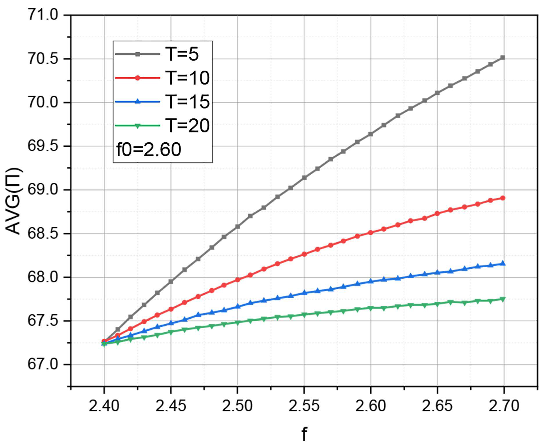
Taking into account the paired representation of the intensity of processing of received requests by the system, it is of interest to determine the dependence (10) variant for $f_0=2.60$, $f\in \left[2.4,2.7\right]$ and $T=\left\{5,10,15,20\right\}$. The calculation results are visualized in Figure 2 and

Table 2. The exact values of the dependencies are presented in Figure 2.

$\mathit{f}$	$\overline{\mathbf{\Pi }}$ $\mathbf{at} \mathit{T}=5$	$\overline{\mathbf{\Pi }}$ $\mathbf{at} \mathit{T}=10$	$\overline{\mathbf{\Pi }}$ $\mathbf{at} \mathit{T}=15$	$\overline{\mathbf{\Pi }}$ $\mathbf{at} \mathit{T}=20$
2.40	67.25968	67.26651	67.23918	67.23918
2.41	67.40319	67.33485	67.29385	67.25968
2.42	67.5467	67.41002	67.33485	67.29385
2.43	67.68337	67.49203	67.38269	67.31435
2.44	67.82005	67.5672	67.43052	67.34169
2.45	67.94989	67.63554	67.47153	67.37585
2.46	68.08656	67.71071	67.51253	67.40319
2.47	68.20957	67.77904	67.5672	67.42369
2.48	68.33941	67.84738	67.59453	67.44419
2.49	68.46241	67.90888	67.62187	67.46469
2.50	68.57859	67.97039	67.66287	67.48519
2.51	68.70159	68.02506	67.70387	67.50569
2.52	68.79727	68.09339	67.73121	67.5262
2.53	68.92027	68.1549	67.75854	67.5467
2.54	69.02278	68.20957	67.78588	67.55353
2.55	69.13895	68.26424	67.82005	67.57403
2.56	69.24146	68.31891	67.84055	67.5877
2.57	69.3508	68.36674	67.86105	67.60137
2.58	69.43964	68.41458	67.88838	67.61503
2.59	69.54897	68.46925	67.92255	67.63554
2.60	69.63781	68.51025	67.94989	67.6492
2.61	69.74032	68.55125	67.97039	67.6492
2.62	69.84966	68.59909	67.98405	67.6697
2.63	69.93166	68.64692	68.01139	67.68337
2.64	70.0205	68.67426	68.03189	67.68337
2.65	70.10934	68.72893	68.05239	67.69704
2.66	70.19134	68.76993	68.06606	67.71754
2.67	70.27335	68.8041	68.09339	67.71071
2.68	70.35535	68.83827	68.12073	67.73121
2.69	70.43736	68.87927	68.1344	67.73121
2.70	70.51253	68.90661	68.1549	67.75171

.

Now let us determine the dynamics of changes in the values of the characteristic (10) variant from the threshold $T\in \left[2,16\right]$ at $f_0=2.60$ and $f=\left\{2.50,2.60,2.70\right\}$. The calculation results are visualized in Figure 3 and

Table 3. The exact values of the dependencies are presented in Figure 3.

$\mathit{T}$	$\overline{\mathbf{\Pi }}\left(\mathit{T},\mathit{f}=2.50\right)$	$\overline{\mathbf{\Pi }}\left(\mathit{T},\mathit{f}=2.60\right)$	$\overline{\mathbf{\Pi }}\left(\mathit{T},\mathit{f}=2.70\right)$
2	69.21277	70.94894	72.54894
3	69.22979	71.02553	72.68511
4	69.24681	71.08511	72.80426
5	69.26383	71.12766	72.90638
6	69.26383	71.17021	73
7	69.27234	71.20426	73.08511
8	69.28085	71.2383	73.14468
9	69.28936	71.26383	73.20426
10	69.30638	71.28936	73.2383
11	69.31489	71.30638	73.27234
12	69.31489	71.31489	73.31489
13	69.3234	71.33191	73.34894
14	69.3234	71.33191	73.34894
15	69.3234	71.34894	73.38298
16	69.3234	71.36596	73.40851

.

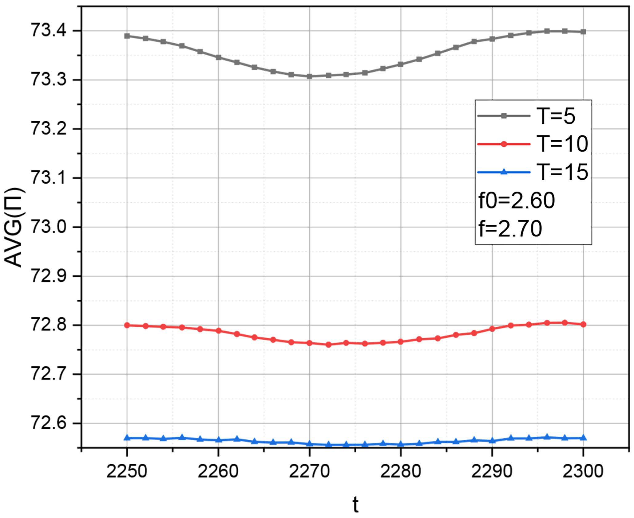
Finally, let us determine the dynamics of changes in the values of the characteristic (9) variant for the time interval $\left[t,t+\overline{t}\right]=\left[2250,2300\right]$ with $f_0=2.60$ and $f=2.70$. The calculation results are visualized in Figure 4 and

Table 4. The exact values of the dependencies are presented in Figure 4.

$\mathit{t}$	$\mathbf{\Pi }\left(\mathit{t},\mathit{T}=5\right)$	$\mathbf{\Pi }\left(\mathit{t},\mathit{T}=10\right)$	$\mathbf{\Pi }\left(\mathit{t},\mathit{T}=15\right)$
2250	73.38927	72.79983	72.56985
2252	73.3843	72.79826	72.56998
2254	73.37761	72.79669	72.56841
2256	73.36923	72.79512	72.57025
2258	73.35745	72.79186	72.56698
2260	73.34566	72.78858	72.56542
2262	73.33557	72.78191	72.56726
2264	73.32548	72.77523	72.56228
2266	73.3171	72.77025	72.56072
2268	73.31043	72.76528	72.56085
2270	73.30715	72.76372	72.55758
2272	73.309	72.76044	72.55601
2274	73.31084	72.76399	72.55615
2276	73.31438	72.76243	72.55629
2278	73.32304	72.76426	72.55813
2280	73.33168	72.7661	72.55656
2282	73.34205	72.77135	72.5584
2284	73.35411	72.77319	72.56194
2286	73.36617	72.78013	72.56208
2288	73.37823	72.78368	72.56562
2290	73.38348	72.79234	72.56406
2292	73.39043	72.79929	72.5693
2294	73.39568	72.80112	72.56944
2296	73.39922	72.80467	72.57127
2298	73.39935	72.8048	72.56971
2300	73.39778	72.80154	72.56985

.

The format of the presentation of calculations of characteristics (9), and (10) by a set of two-dimensional functions presented in Figure 1, Figure 2, Figure 3 and Figure 4, chosen for clarity and taking into account the fact that characteristics (9), and (10) are functions of four variables, which makes its graphical interpretation on a static medium impossible. The change ranges of characteristic parameters (9) and (10) are selected in such a way as to simplify the comparison of the obtained results with analogs (proving the adequacy of the mathematical apparatus presented in Section 2) and to demonstrate specific features of the dynamics of characteristics (9), (10) that deserve special attention (see Section 4).

4. Discussion

Let us recall the results of the review presented in Section 1. In particular, the work [27] is semantically closest to the author’s research. The authors of article [27] model the functioning of the computing unit of the Data Center with an emphasis on determining the energy efficiency of the first. As a model of the computing unit, the authors of the mentioned article propose a $M|M|1|\infty$ queuing system taking into account the single-threshold energy consumption management policy. At the same time, in the article [27], it is assumed that both the intensity of requests to the model and the intensity of their processing by the system do not depend on time (for a Data Center with a consistently high load on its computing units, this assumption is perceived as natural). In the article [27], we are primarily interested in the results of computational experiments, namely, the dependence of the average energy consumption of the computing unit in the stationary mode $\overline{\mathsf{\Pi }}$ on the threshold $T$, the basic clock frequency $f_0$ and the increased clock frequency $f$ at the determined stable parameters of the metric (7), i.e., $\left\{C,U,{\mathsf{\Pi }}_s\right\}$.

In the experiments, the results of which are presented in Section 3, we used similar values of both the fixed parameters of the metric (7) and similar ranges of changes of the controlled parameters, i.e., $\left\{T,f,f_0\right\}$. Our choice was aimed at simplifying the substantiation of the adequacy of the mathematical apparatus presented in Section 3. As shown in Figure 1, Figure 2 and Figure 3, dependencies are generated by our model in a time-normalized form. As expected, the results of the calculation of the variants of dependence $\overline{\mathsf{\Pi }}\left(f_0,f,T\right)$ carried out based on the author’s model of type $M\left(t\right)|M\left(t\right)|1|\infty$ in a time-normalized form (Figure 1 and Figure 2), are extremely close to the semantically identical dependencies presented in the analog [27] (Figures 2a and 3a in [27], respectively). This allows us to draw an inductive conclusion that the author’s concept of the energy efficiency assessment of the Edge Computing infrastructure peripheral server functioning over time is adequate.

Separately, we note that the mentioned analog (the $M|M|1|\infty$ model of the computing unit taking into account the energy consumption policy $T$) cannot be used for the object we are researching, i.e., the process of functioning of the Edge Computing infrastructure peripheral server because the latter is characterized by the need for periodic peak computing power (survey of the sensor network, initial real-time processing of received data and sending a report). The model [27] is simply not able to account for these spikes. It was this fact that prompted us to consider the intensity of the arrival of new requests to the model and the intensity of the processing of accepted requests by the system as non-random functions of time while preserving the interpretation of the research object as a birth-and-death Markov process. The mathematical apparatus presented in Section 2 is focused on determining time-uniform estimates of the approximation error of the original Markov multiparameter process using processes with a lower number of states. This approach makes it possible to determine the value of the sought probabilistic characteristics of the initial weak ergodic process with the required accuracy on a representative time interval.

Now let us interpret the characteristic trends that follow from the graphs presented in Section 3. Let us pay attention to Figure 1. It can be seen that an increase in the base clock frequency $f_0$ leads to a synchronous monotonic increase in the average power consumption $\overline{\mathsf{\Pi }}$ (which is accompanied by a decrease in the service waiting time for requests accepted by the model). However, with a decrease in the value of $f_0$, the rate of decrease in energy consumption $\overline{\mathsf{\Pi }}$ is different and depends on the value of the threshold $T$. This circumstance makes it possible to predict the possibility of setting the problem of determining the optimal value of the threshold $T$ to minimize the power consumption of the peripheral server in standby mode when the algorithmic-logical complex of the latter operates at the frequency $f_0$.

Figure 2 shows that an increase in the clock frequency $f$ leads to an increase in the power consumption of the peripheral server. Manipulation of the threshold value $T$ affects only the intensity of growth of the graphs, but not the overall trend. But note that these graphs are obtained for a fixed value of $f_0=2.60$, while $f\in \left[2.40,2.70\right]$. The situation $f<f_0$ was not considered in the formalization of the energy consumption management policy, but the model shows signs of survivability, the limits of which can be further explored.

Graphs from Figure 3 confirm those determined about Figure 2 trends. It can be seen that the decisive influence on power consumption $\overline{\mathsf{\Pi }}$ causes the increase in the clock frequency $f$. Threshold value $T$ causes a noticeable effect on power consumption only when parameters $f_0$, $f$ are close in value. This circumstance allows us to state that the classic version of the energy consumption management $T$ policy does not reveal its full potential in the context of the research object. Taking into account this fact, the authors consider it promising to switch to an interval interpretation of the parameter $f$. Moreover, the author’s mathematical apparatus allows for setting up and solving related optimization problems with sufficient computational efficiency.

The results presented in Figure 4 show that over time, the value of energy consumption goes to the corresponding limit value, which depends on the value of the threshold $T$ at fixed values of the parameters $f_0$, $f$. This unequivocally confirms the fundamental suitability of the $T$ policy for power consumption management of the peripheral server as an important link of the Edge Computing infrastructure. It was the use of the author’s mathematical apparatus that made it possible to obtain objective confirmation of this. We also note that the influence of the periodic nature of the intensity functions (11) on the level of energy consumption decreases with the increase in the value of the threshold $T$.

Also, note that our goal was to provide engineers with a simple and adequate metric for estimating the power consumption of a functioning edge server both at an arbitrary moment in time and for a certain time interval. It is this goal that determines both the compactness of the final metric (9) and (10) and the simplicity of the parametric representation of a rather mathematically complex queuing system $M\left(t\right)|M\left(t\right)|1|\infty$ in it.

5. Conclusions

Edge computing is a viable solution for organizations whose activities involve real-time data processing. A solution in the distributed computing paradigm can provide numerous benefits, including improved performance, increased security, and reduced latency. At the same time, computing resources at the edge of the network are limited compared to the central cloud server’s power. This circumstance actualizes the problem of ensuring the energy efficiency of computing on the peripheral server as the edge computing infrastructure basic unit.

The material of the article is devoted to the research of the peripheral server energy consumption managing process defined based on the threshold policy by manipulating the values of the characteristic parameters of the arithmetic-logical complex of the latter. The research object is formalized by a Markov queue model with a single-threshold control scheme for the intensity of accepted requests service. A characteristic feature of the life cycle of a peripheral server is the non-stationary mode of operation in terms of energy consumption, due to the need to periodically poll the controlled sensor network and process the received data in real-time. To take into account this circumstance, the intensities of transitions in the heterogeneous birth-and-death Markov process of the created model are interpreted as non-random periodic functions of time. An approach for determining time-uniform estimates of the approximation error of the original weakly ergodic multiparameter Markov process using processes with a smaller number of states is proposed. Using this approach, the main probabilistic characteristics of the research object are analytically determined with the necessary accuracy on a representative time interval. The adequacy of the created mathematical apparatus is substantiated based on the closest semantically analog.

A computational experiment on estimating the energy consumption of a peripheral server instance in time proved the functionality of the created mathematical apparatus. The discussion of the experiment results made it possible to outline a whole list of directions for promising further research, in particular:

−

setting the problem of determining the optimal value of the energy policy threshold to minimize the power consumption of the peripheral server in standby mode;

−

It was experimentally confirmed that the created model shows signs of survivability when the values of the controlled parameters exceed the established limits. The search and analysis of the origins of this survivability is a promising research task;

−

There are signs of a promising transition to interval interpretation of individual characteristic parameters of the created model. This thesis needs research.

The mathematical apparatus proposed in the article was evaluated taking into account simplified and synthetic query distributions. Based on the recommendation of a respected reviewer, the authors are going to devote the next work to conducting a series of experiments to evaluate, using the tools proposed in the article, the functioning processes of real EDGE systems containing peripheral servers with various scenarios for receiving data from sensor networks