Article

Research on Mixed Matrix Estimation Algorithm Based on Improved Sparse Representation Model in Underdetermined Blind Source Separation System

School of Electrical and Electronic Engineering, USM Engineering Campus, Universiti Sains Malaysia, Nibong Tebal 14300, Malaysia
*
Author to whom correspondence should be addressed.
Electronics 2023, 12(2), 456; https://doi.org/10.3390/electronics12020456
Submission received: 7 December 2022 / Revised: 8 January 2023 / Accepted: 11 January 2023 / Published: 15 January 2023
(This article belongs to the Section Circuit and Signal Processing)

Abstract

:
The estimation accuracy of the mixed matrix is very important to the performance of the underdetermined blind source separation (UBSS) system. To improve the estimation accuracy of the mixed matrix, the sparsity of the mixed signal is required. The novel fractional domain time–frequency plane is obtained by rotating the time–frequency plane after the short-time Fourier transform. This plane represents the fine characteristics of the mixed signal in the time domain and the frequency domain. The rotation angle is determined by global searching for the minimum L1 norm to make the mixed signal sufficiently sparse. The obtained time–frequency points do not need single source point detection, reducing the calculation amount of the original algorithm, and the insensitivity to noise in the fractional domain improves the robustness of the algorithm in the noise environment. The simulation results show that the sparsity of the mixed signal and the estimation accuracy of the mixed matrix are improved. Compared with the existing mixed matrix estimation algorithms, the proposed method is effective.

1. Introduction

Blind source separation (BSS) is very popular in engineering applications because it only uses mixed signals to separate source signals without prior known conditions.
In practical application, underdetermined blind source separation (UBSS) has become a research hotspot because the number of source signals is more than that of receiving sources, which is more in line with the scene of practical application.
At present, the main method to solve UBSS is sparse component analysis (SCA) [1], which was the first proposed in 2000 by Lewicki to use the super complete sparse representation based on the maximum a posteriori probability to obtain the sparse feature of the signal and realise the restoration of sparse source signals. Given that the number of source signals is larger than the number of microphones, the unique deterministic solution cannot be obtained for UBSS, and the dimensional reduction is realised by obtaining the sparse representation of the mixed signal, thereby acquiring the deterministic solution.
In 2001, Bofill and Zibulevsky proposed a ‘two-step method’ based on SCA [2]: one step is to estimate the mixing matrix, and the other is to separate the source signal. This idea to achieve UBSS has been recognised and used by many scholars, which has generated much research [3,4,5,6,7,8,9,10,11,12,13,14,15,16,17]. In this paper, considering that the estimation accuracy of the mixing matrix directly determines the accuracy of the separated source signal, the research on the first step, that is, estimating the mixing matrix, is taken as our key research object.
Two points need to be considered in the study of mixed matrix estimation.
  • Finding the sparse representation model for the time domain mixed signal
  • Clustering the sparse representation model
In the ‘two-step method’ proposed by Bofill [2], the time domain mixed signal is used to find the sparse representation model of the mixed signal through Fourier transform (FT), and the potential function method is used to cluster to obtain the mixed matrix estimation. The experimental results are ideal but have shortcomings. On the one hand, the amount of data to be processed is too large, and the calculation is complex. On the other hand, the clustering method of the potential function selected by Bofill does not estimate three or more observation signals, which places high requirements on the number of source signals and has limited applications.
In view of the existing shortcomings, many scholars have made improvements [3,4,5,6,7,8]. For example, in the sparse representation model, in 2006, Li, Y. et al. [3] analysed how to use the sparsity of the signal to represent the observed signal completely and improve the linear clustering characteristics of the observed signal, but the implementation steps were not given. In 2007, M. X. et al. [4] proposed the time domain retrieval average method that can be used to estimate the mixing matrix. This method requires that each source signal has enough single-source interval data for estimating the mixing matrix. However, most signals do not meet this condition in the time domain, so they are not very useful for UBSS. In the same year, Kim, S. et al. [5] used signal sparsity [3] to achieve the single source point (SSP) detection of signals to improve the clustering directivity of data points. At a certain time, only one time–frequency point has a large energy value, and the other values are approximately zero, to discard some data points that affect clustering and detect useful points. However, in practical applications, due to the interference and other irresistible factors, useful points are often discarded, and invalid points such as noise are used as SSPs, which has a great effect on the clustering results. Therefore, there is much research on improving SSP [6,7,8]: Ref. [6] proposed a singular value decomposition method to solve the mixed vectors corresponding to different sets of SSPs to relax the conditions of existing methods for time–frequency single-source areas. Ref. [7] proposed using local stationarity and distribution symmetry to reduce pseudo SSPs. Ref. [8] used low noise points to remove the influence of noise. Although these algorithms improve the detection of SSP, the gains and losses are not worth the losses because the computational load is greatly increased again, which is contrary to the original intention of SSP detection.
In addition, some scholars try to find a better sparse representation model for time domain mixed signals through other transformations, such as in the paper [9,10,11,12]. In [9], a lp (0 < p ≤ 1) regularisation was provided to reconstruct the sparse sources, in which p can be dynamically selected to achieve the best performance. The experimental results demonstrate the robustness of the proposed method to room reverberation under various speech separation cases compared with conventional methods. However, this algorithm involves too much computation.
In [10], the author used wavelet transform to replace short-time Fourier transform (STFT) because wavelet transform inherits and develops the idea of STFT localisation, overcomes the shortcomings of window size not changing with frequency and can provide a ‘time–frequency’ window that changes with frequency. The time and frequency information of the signal can be observed simultaneously, which is beyond the reach of FT. However, wavelet transform also has limitations, that is, the redundancy is very large, which brings much useless work.
Fractional Fourier transform (FrFT) is selected to replace STFT to find the best sparse representation model of the observed signal [11,12,13,14,15]. The purpose of FrFT is the same as that of wavelet transform. It tries to find a transform that reflects the information of the signal in the time domain and frequency domain at the same time. However, FrFT is different from the commonly used quadratic time–frequency distribution. It uses a single variable to represent time–frequency information without cross term problems. In [11], the observed signal is subject to FrFT, and the mixed signal is separated in the fractional domain. In this paper, the selection of the rotation angle is not based on the sparse model of the mixed signal, so the separation characteristics need to be improved.
In [12], Long et al. first proposed the concept of the fractional low order space time–frequency matrix, improved pseudo Wigner–Viile using fractional low order moments and studied blind separation technology based on it. This algorithm systematically demonstrates the advantages of fractional time–frequency space over UBSS, which can not only improve the time–frequency point aggregation characteristics of signals but also have good performance in noisy environments. Through the research of Long et al., the following researchers focus on the fractional time–frequency space. Long et al. verified the advantages of the time–frequency space in the fractional domain but did not provide a specific method to obtain the time–frequency space in the fractional domain.
In [13], Wang et al. proposed distinguishing signals in the fractional domain by using the sparse feature of the fractional domain. After FrFT, the signal amplitude shows compressibility with the transformation of order. The main information is extracted through the algorithm proposed by Wang et al., which is divided into the main information domain and the secondary information domain. The complementary information of the two are fused to form a mixed amplitude feature, and then the mixed amplitude feature, real part feature and imaginary part feature are fused. Finally, the fractional domain features of different orders are fused to achieve face recognition, which also provides an idea for the study of non-stationary signals in this paper.
In [14], Yao et al. used FrFT to convert the mixed signal into fractional Fourier domain firstly and estimate the noise power spectrum. In the optimal order domain, they used spectral subtraction to remove noise from the mixed signal and the fast-Independent Component Analysis (fastICA) algorithm to perform blind separation and smooth filtering on the mixed signal. The simulation results show that the separation effect is superior, but the algorithm is only suitable for BSS, not for the UBSS in this paper.
In [15], the observed signal was transformed into FrFT based on sparsity, and the residual removal of FrFT energy aggregation and sparse decomposition was used to suppress noise and reverberation interference. Through the fusion of features in the multiorder FrFT domain, the separability between targets was increased, and then the target classification in a specific environment was realised. However, the algorithm was carried out in a specific environment, and the global threshold was used to search the fractional transformation order, which required a large amount of computation.
Moreover, many scholars [16,17] opted to improve the clustering method in addition to improving the sparse representation model.
Zhen et al. [16] used SSP for adding the mixture TF vectors whose sparse coding coefficient vector contains only one non-element into Ω. Then, the hierarchical clustering algorithm was used to cluster the data points that meet the requirements, and single source vectors with dominant energy were grouped to achieve mixed matrix estimation. In this algorithm, improved SSP is used to reduce the calculation amount greatly and increase the clustering characteristics of time–frequency data points. Then, the hierarchical clustering algorithm is selected to achieve high-quality clustering without setting initial values such as the K-means algorithm and then improve the accuracy of mixed matrix estimation. However, for the hierarchical clustering algorithm, high-quality clustering is based on global clustering, which is bound to include clustering of some pseudo SSP points, which places high requirements for the SSP algorithm. Pseudo SSP is not discussed in this paper, resulting in the limited precision of mixed matrix estimation in this paper.
He et al. [17] used SSP and the density-based spatial clustering of applications with noise (DBSCAN) method to achieve mixed matrix estimation. In this algorithm, He et al. used SSP detection to enhance the linear clustering characteristics of sparse signals. Then, they used DBSCAN to search high-density points and constantly connect adjacent data to form clusters, and automatically find the number of clusters and corresponding cluster centres. Each cluster centre corresponds to a column vector of the underdetermined mixed matrix to estimate the mixed matrix. This algorithm skilfully uses SSP to enhance the clustering characteristics, and DBSCAN searches for the cluster centre. However, in UBSS, the number of clusters that DBSCAN clustering algorithm searches for often generates large errors due to the presence of interference, which greatly affects the accuracy of mixed matrix estimation.
Furthermore, many algorithms focus only on the selection of clustering methods [18,19,20,21]; in [18], K-means is selected to cluster time–frequency points, but K-means is particularly vulnerable to the effect of the initial cluster centre and falls into the problem of the local optimal solution. In [19], the particle swarm optimisation (PSO) algorithm was selected to achieve clustering. The advantage of this algorithm is that the initial value setting is simple, the number of source signals can be well determined, and the mixed matrix estimation accuracy can be improved. However, the largest problem of this clustering algorithm is that it is often unable to converge globally. Considering that UBSS is an estimation of direction, by improving the traditional fuzzy C-means [18], the directional C-means (DFCM) clustering method [21] is adopted to estimate the number of source signals before realising the mixed matrix estimation. DFCM is more robust to UBSS, but this algorithm is easy to be interfered with by outliers and requires very high time–frequency points, which affects the accuracy of mixed matrix estimation.
For the above contents, the research summary of the mixing matrix in recent years is shown in Table 1:
To sum up, there is much research on mixed matrix estimation, and the estimation accuracy of mixed matrix is increasing. However, some problems remain:
  • It is easy to be interfered with by outliers, resulting in the low estimation accuracy of mixed matrix.
  • The amount of the calculations is too large to be applied in UBSS.
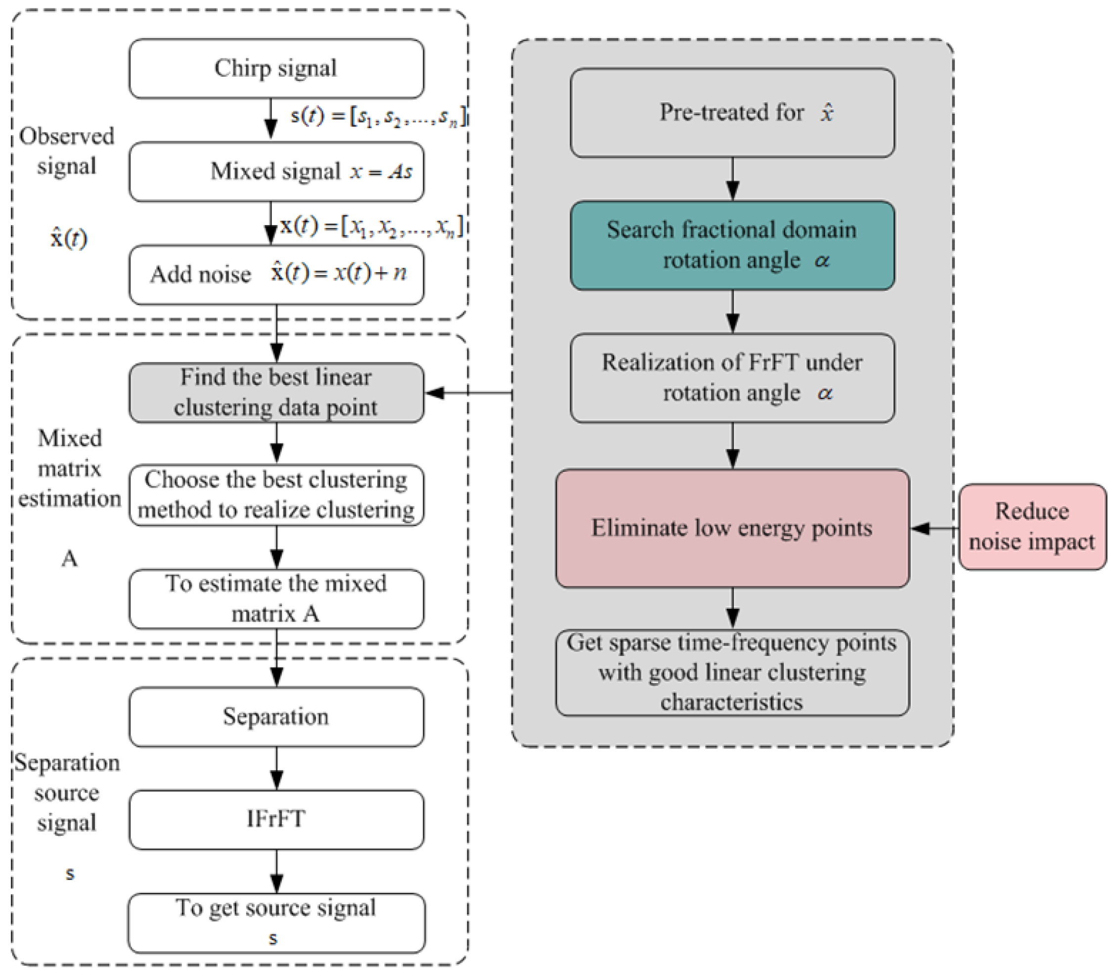
To improve the performance of the algorithm in noisy environments, reduce the effect of interference and make the computational complexity more moderate, this paper tries to rotate the static time–frequency plane to obtain FTs at different angles. The rotation angle (which can be any angle) is the free parameter in the FrFT. Through the FrFT of different orders, that is, the rotation of the signal at different angles on the time–frequency plane, all the characteristics of the signal from the time domain to the frequency domain can be obtained, and then the detailed characteristics of the time–frequency change of the signal are reversed to obtain the required finer characteristic information [11,12,22]. The characteristic information can be used to find the sparse representation of the mixed signal.
The contribution of this paper is to select FrFT creatively to rotate the time–frequency plane, find the fractional domain where the observation signal is sufficiently sparse and remove the pseudo SSPs in the fractional domain. Thus, the time–frequency points in the fractional domain are fully clustered without the need of SSP detection, obtaining a high estimated mixed matrix column vector. In addition, the insensitivity of the fractional domain to noise improves the suppression of noise in mixing matrix estimation.

2. Proposed Method

For the UBSS system with N source signals and M channels:
x ( t ) = A s ( t ) + n
where x t = x 1 t , x 2 t , , x m t is the mixed signal observed in time domain, A = a 1 , a 2 , , a n is the mixing matrix of [M × N] and s t = s 1 t , s 2 t , , s n t is the time–domain source signal we want to separate. n is the noise in the system. The N-channel source signals form M-channel mixed signals through the mixing matrix. Our purpose is to separate the source signals from the mixed signals in the UBSS system. The accuracy of the mixed matrix estimation directly determines the separation performance of the UBSS system, and the character of linear clustering is the basis of estimating the mixed matrix. Therefore, this paper aims to find the best linear clustering data point for analysing the estimation of the mixed matrix A.
In recent years, STFT was generally used to find linear clustering points for time domain mixed signals. Although the linear clustering characteristics of time–frequency points have been improved after STFT transformation, the clustering characteristics are still not evident for many data signals, resulting in inaccurate estimation of the mixing matrix and too much noise effect.
Combined with the introduction of the fractional Fourier transform, this paper attempts to find the parameters α in the fractional Fourier transform, then the fractional Fourier transform is implemented for the time-domain mixed signal so as to obtain more sparse time-frequency points, improve the time-frequency point clustering characteristics of the signal and achieve the purpose of improving the estimation accuracy of the mixed matrix. Simply understood, it is to transform the mixed signal into a rotated time-frequency plane, which can make the data points show more obvious linear clustering characteristics. This system is the α-UBSS proposed in this paper. The algorithm flow chart is shown in Figure 1. In this algorithm, because the fractional domain transformation is not sensitive to noise [23], the noise appears as low energy points in the fractional domain, and the low energy points can be removed to achieve the purpose of noise removal. In summary, using this algorithm, the linear clustering characteristics are increased, whereas the influence of noise is reduced.
To study the fractional domain UBSS, firstly, the fractional domain FT is briefly introduced.

2.1. Theory of Fractional Fourier Transform (FrFT)

Firstly, different from the existing algorithms, FrFT is performed on the mixed signal due to the following the reason:
Analysis is made from the definition of FT. It is defined from different angles for FT [23].
The integral form is
F π 2 f t = 1 2 π exp j u t f t d t
In (2), f t is the time domain signal, F π 2 is the FT operator, t represents the time domain variable and u represents the transformation domain variable.
The form defined by the characteristic function is
  F π 2 ϕ n t = e j n π 2 ϕ n u   ϕ n t = exp t 2 2 H n t H n t = 1 n e t 2 d n d t n e t 2
In (3), ϕ n is the characteristic function, and the FT operator F π 2 is defined by the Hermite characteristic function. (2) and (3) are equivalent, that is, the FT operators F π 2 of (2) and (3) are the same.
To extend the FT form to the general form, the fixed value of π 2 in Formula (3) is replaced by the general angle α, and the definition of FrFT is obtained:
F α ϕ n t = e j n α ϕ n u
Euler formula simplification obtains
F α f t = 1 j c o t α 2 π exp j c o t α 2 t 2 + j c o t α 2 u 2 j u t s i n α f u d t
when α = π/2, and Formula (5) is the definition of FT (2). FrFT is a generalisation of FT. When α → 0, FrFT degenerates into the time domain.
F α 0 f t = f u
The above analysis verifies the unified time–frequency characteristic of FrFT. The fractional Fourier domain can be understood as rotating the time–frequency plane obtained by FT by a certain angle [24]. This plane integrates the information of the time domain and frequency domain. Compared with the static time–frequency plane obtained by FT, the fractional domain can more accurately characterise the characteristics of time domain and frequency domain, and is more suitable for the blind source separation system (without prior known conditions). Although STFT realises time–frequency display by adding a window to FT, the fixed window makes the time–frequency resolution not too high. To improve the window, it needs to pay the cost of computing, so this paper chooses FrFT to implement BSS. In addition, the insensitivity of FrFT to noise is another important reason for choosing it [25,26,27,28,29].
For the time–frequency domain UBSS system with a specific rotation angle,
X α t , k = A S α t , k = m = 1 M a m s α , m t , k
X α t , k   is the coefficient of FrFT of the time domain source signal x(t) at the time–frequency point of time–frequency point (t, k) in the fractional domain, S α t , k   is the coefficient of FrFT of the time domain source signal s(t) at the time–frequency point (t, k), a m   is the m-th column vector of the mixed matrix A and α is the rotation angle of FrFT.

2.2. Transformation Order Determination to Obtain Sparse Representation Model

To extend the research of UBSS sparse signals from the Fourier domain to fractional domain, the Fourier domain needs to rotate a certain angle to the fractional domain. The most important thing is to determine the rotation angle first. Different rotation angles correspond to dissimilar properties of the fractional domain. In UBSS, this research focuses on the sparsity of mixed signals in the fractional domain. In recent years, the commonly used method for sparsity measurement is L1 norms [9]. Thus, in this paper, this idea is innovatively applied to α-UBSS, and L1 norms of data points obtained are compared under different α rotation angles. The minimum value of L1 norms is the sparsest data point [30], and the time–frequency domain obtained under the corresponding α rotation angle is the sparsest representation model of mixed signals we are looking for. (Note: In FrFT, α is the rotation angle and p is the transformation order. π 2 p = α .)
Through the above analysis, this paper uses L1 norm as a sparse measure to determine the optimal transformation order in the fractional domain.
The mixed speech signal is expressed as
x t = x 1 t , x 2 t , , x N t T
After α order of FrFT, x(t) is expressed as F α x = F X . The L1 norm of FrFT of the mixed speech signal is (10) according to L1 norm expression (9):
x 1 = i = 1 N x i
L 1 = F X 1 = i = 1 N F X i
Finally, the transformation order corresponding to minimising the L1 norm value is searched, that is, the sum of all vector element values corresponding to the mixed signal is the smallest, as shown in (11):
α = min L j   j = 1 , 2 , , J
j represents the number of all elements contained in the fractional domain mixed signal vector.
To complete the global α search one by one, the computation is too much. Chu’s [31] algorithm is used to obtain the optimal order based on the combination of step rough search and step exact search. In the rough search, a step size of 0.01 is chosen, and in the exact search, a step size of 0.0001 is selected. In this way, the search accuracy and the calculation amount can be ensured moderate. The algorithm flow chart is shown in Figure 2.

2.3. Clustering for Mixing Matrix Estimation

Thus far, the sparsity analysis of mixed signals has been extended to a more generalised time–frequency plane. Then, how about the clustering characteristics of signals in this plane? Can the mixed signals show evident differences? The answer is yes.
To make the signal points have sufficient clustering characteristics, in STFT, SSP detection is firstly performed on the time–frequency point. On any time–frequency point (t, k) in the fractional domain, the real and imaginary parts of the observed signal X α t , k are
R X α t , k = m = 1 M a m R S α , m t , k
I X α t , k = m = 1 M a m I S α , m t , k
Compared with Formula (5), the real part of the observation signal does not change, whereas the coefficient of the imaginary part is determined by the rotation angle. Given the addition of the rotation angle, it is not sensitive to the noise and gathers the energy of the observed signal [32,33], so that some pseudo SSPs that would have been detected as SSPs in STFT would not be detected as the noise background in the fractional domain. Thus, sufficient sparsity can be realised without SSP detection. For the sample point k in any fractional domain, only one source S α , i k   i = 1 , 2 , , m   is a nonzero value, and other sources S α , j k ( i j ) are all zero values, that is
X α , 1 k a 1 i = X α , 2 k a 2 i = = X α , n k a m i = S α , i k
Thus far, the estimation of the mixing matrix has been transformed into solving Equation (14), and each solution corresponds to a column vector of the mixing matrix, a i = a 1 i , a 2 i , , a m i T .
To sum up, the mixed matrix estimation algorithm (Algorithm 1) proposed in this paper is as follows:
Algorithm 1: estimate mixing matrix algorithm steps
Input: observation   signal   x ^ ( t ) = [ x ^ 1 ( t ) , x ^ 2 ( t ) , , x ^ m ( t ) ]
  • Using chirp signal to simulate non-stationary signal as source signal input. s ( t ) = [ s 1 , s 2 , , s n ]
  • Using rand (m, n) of MATLAB to random generate mixed matrix.
  • Obtaining mixed signal. x = A * s
  • Adding noise to the mixed signal to simulate the actual scene. x ^ ( t ) = x ( t ) + n
Process: estimate the mixing matrix A
  • Find the best linear clustering data point
    (1)
    Pre-treated for x ^ ; standardise, to make the data conform to the distribution with mean value of 0 and variance of 1 through transformation
    (2)
    Search fractional domain transformation order p   ( π 2 p = α )
    • Obtain p1 (transformation order) by rough search
      • dp = 0.01; define the rough search step
      • p1 = -1:dp:0; achieve global search from [−1, 0]
      • for i = 1:length(p1)
      • xaf1(i,:) = frft(x1,p1(i)); data points obtained after FrFT
      • L(i,:) = norm(xaf1(i,:), 1); use L1norm to realise sparsity measurement
      • L1 = min(L); find the transformation order corresponding to the sparse time-frequency point
    • Obtain p2 (transformation order) by exact search
      • dp = 0.0001; define the exact search step
      • p2 = P1-dp:dp^2:P1+dp; search p2 near p1
      • for i = 1:length(p2)
      • xaf2(i,:) = frft(x1,p2(i)); data points obtained again after FrFT
      • L(i,:) = norm(xaf2(i,:), 1); use L1norm to realise sparsity measurement
      • L2 = min(L); find the final transformation order corresponding to the most sparsity time-frequency point
    (3)
    Realisation of FrFT under transformation order p
    (4)
    Remove low energy points; set the threshold value to 0.5, and set the point less than threshold to 0
    (5)
    Obtain sparse time-frequency points with good linear clustering characteristics
  • Choose the best clustering method to realise clustering
  • Each clustering direction vector corresponds to a column vector of the mixed matrix to estimate the mixed matrix A
Output: obtain the estimated mixing matrix A

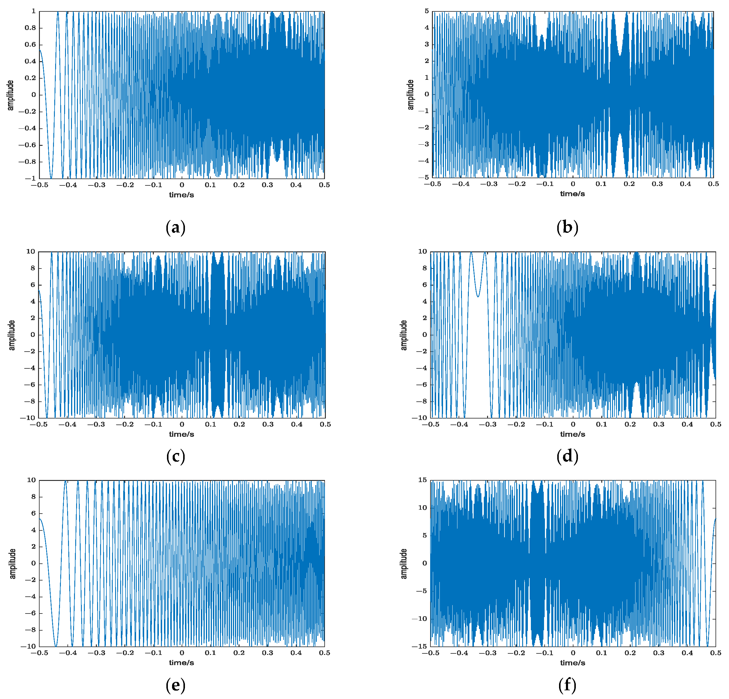
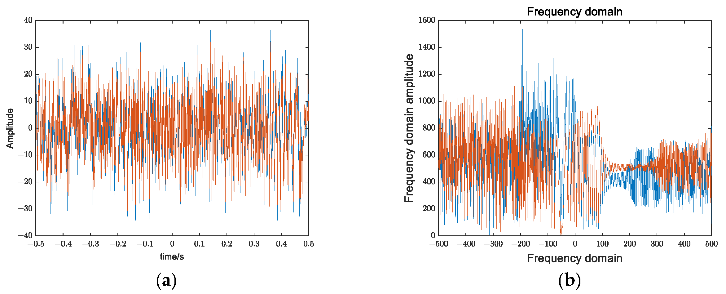
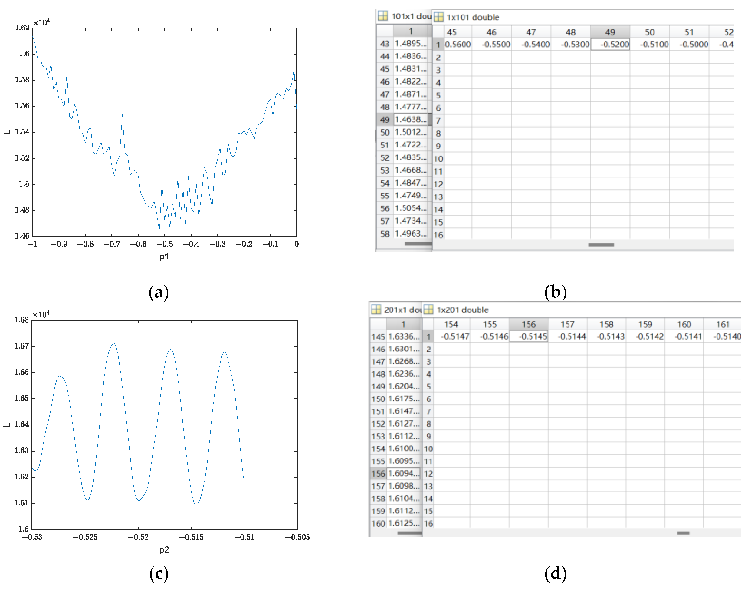
3. Simulation Experiment and Result Analysis

The development environment used in this research is MATLAB R2016b. The computer is configured with i7 CPU and 16 GB RAM, the operating system is Windows 11 and the source signal randomly selects from the consonant data set.
This paper mainly realises the following research:
  • Noise suppression in the fractional domain
  • Optimal transformation order selection
  • Comparison of mixed matrix estimation performance

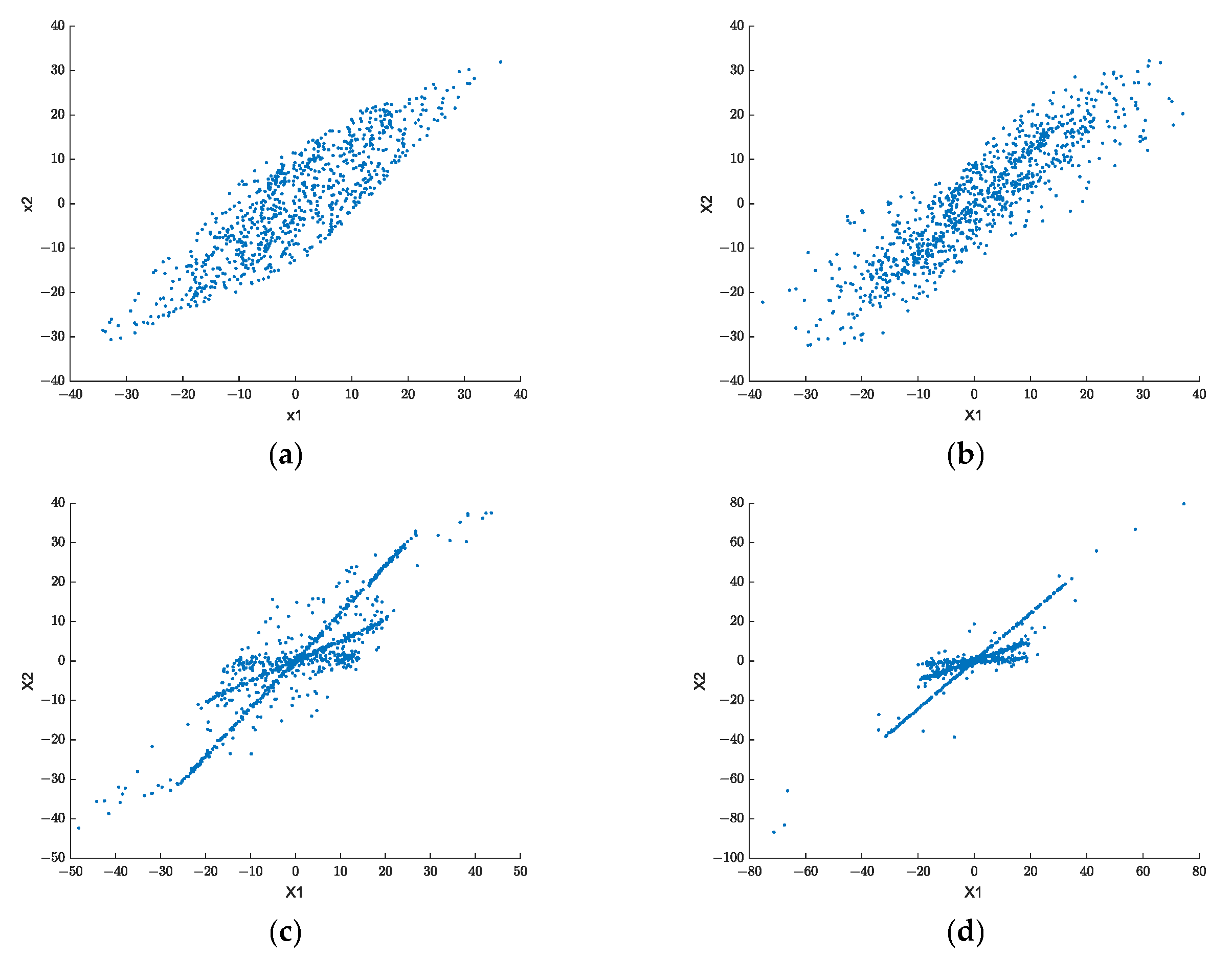
3.1. Noise Suppression in the Fractional Domain

Firstly, the FrFT domain simulation experiment is carried out for single-tone signal and noise to observe the energy accumulation of single-tone signals with different signal-to-noise ratios (SNR) in the whole fractional domain. To observe data easily from the equation, we use   π 2 p = α , α is the rotation angle and p is the transformation order, as discussed in Section 2.1 above. The change from 0 to π 2 of α corresponds to the change of the signal from the time domain to the Fourier domain, and the corresponding p value is [0, 1]. To facilitate observation, the transformation is observed from the Fourier domain to the time domain, that is, α from [− π 2 , 0] and the corresponding p value is [−1, 0], so the whole fractional domain is p from −1 to 0.
Figure 3 shows the energy aggregation of single-tone u that is randomly selected with different SNRs in the fractional domain. Figure 3b–d show the search results of transformation order when SNR is 10 dB, 5 dB and 1 dB, respectively.
The experimental results show that FrFT has a certain energy aggregation to the signal in the transform domain, its energy aggregation is related to the transform order and the energy aggregation is the best under the optimal order. Moreover, FrFT has a certain energy aggregation to the signal in the transform domain. Under the conditions of different SNRs, the energy of speech is relatively concentrated, but the change of the noise bottom is not evident, the energy aggregation of speech is related to the transform order and the energy aggregation is the best under the optimal order.
To verify the suppression of noise in speech signals and design the simulation experiment of speech signals with different SNRs at the same transformation order, the same transformation order is randomly selected for simulation, and the results shown in Figure 3 are obtained. Under the conditions of different SNRs, the energy of speech is concentrated, but the change of the noise bottom is not noticeable. The distinction between a clean signal and noise is increased through FrFT to reduce the influence of noise on system performance in subsequent research of speech separation and achieve the purpose of denoising.
Four groups of speech signals (clean speech signals and noisy speech signals with a signal-to-noise ratio of 10 dB, 5 dB and 0 dB) are subjected to fractional domain FT of the same order (p = 0.9943), as shown in Figure 4:
The simulation and comparison from Figure 3 verify that the fractional domain FT has energy aggregation characteristics for speech signals with different SNRs, and the energy aggregation characteristics are not affected by noise. The advantages of the BSS system in the noise environment in the fractional domain are verified.

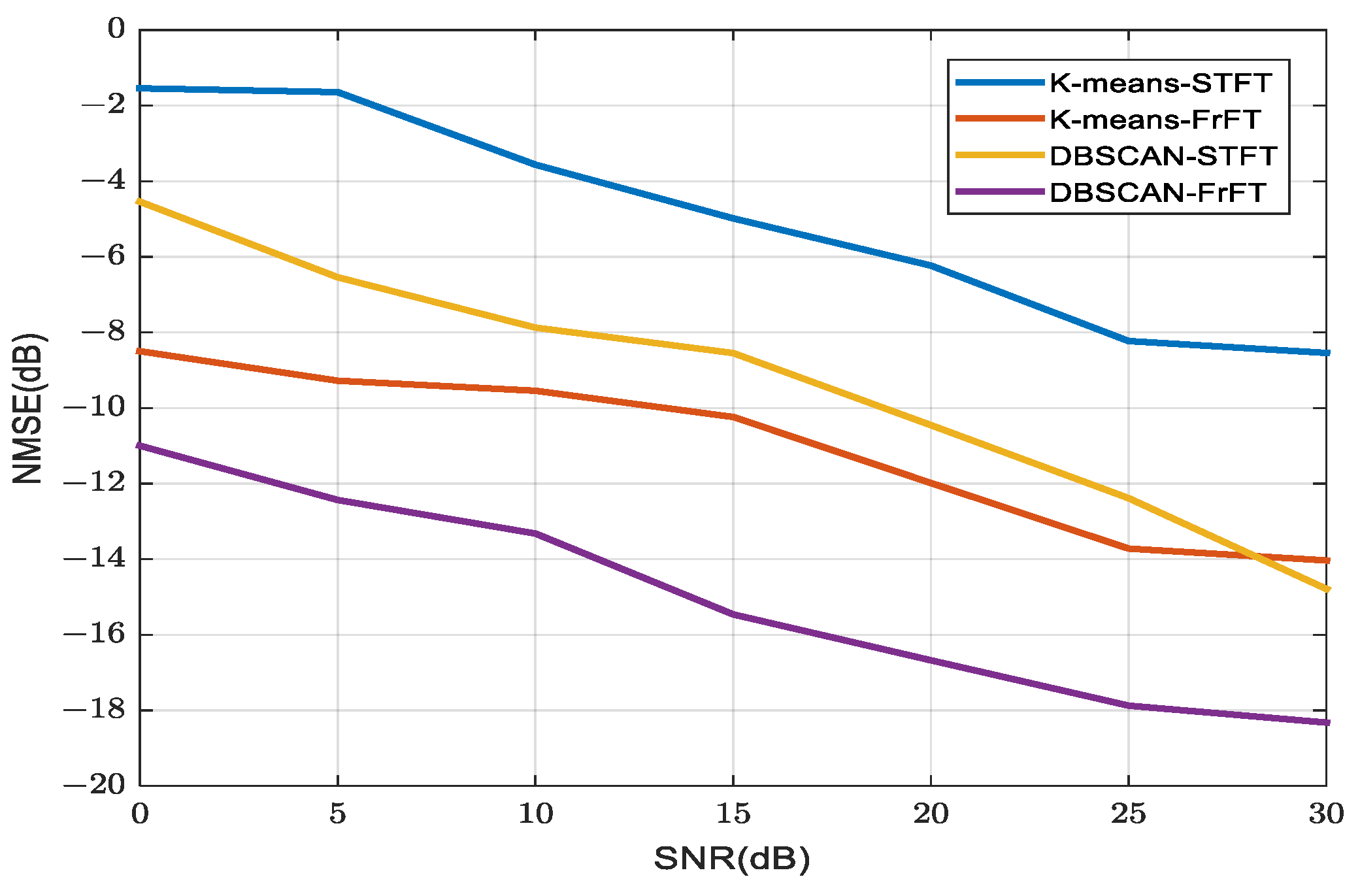
3.2. Comparison of Mixed Matrix Estimation Performance

The estimation performance of the method proposed in this paper is tested on the underdetermined mixing matrix through the MATLAB simulation results. The chirp signal is used to simulate a non-stationary signal, and chirp signals with six different parameters are selected, as shown in Table 2.
The time domain waveform of the six source signals is shown in Figure 5. (The horizontal axis is the sampling sample length, and the vertical axis is the signal amplitude).
Select mixed source signal (m = 2 and n = 6) of UBSS system for simulation. The rand (2, 6) command of MATLAB randomly generates the mixing matrix as follows:
A = [ 0.9572 0.8003 0.4218 0.7922 0.6557 0.8491
   0.4854 0.1419 0.9157 0.9595 0.0357 0.9340]
After the six source signals pass through the mixing matrix A, mixed signals are obtained, as shown in Figure 6:
Next, to realise FrFT for the mixed signal, the transformation order is searched for first. In this paper, the order of transformation is obtained by searching the sparsest transformation domain.
According to the previous analysis, the L1 norm is used as the approximate estimation of signal sparsity in this paper.
Figure 7 shows the change behaviour of sparsity with the change of transformation order.
In a and c of Figure 7, the horizontal axis is the order change, and the vertical axis is the L1 norm value that is used to measure sparsity. A and b are about rough search data and result; c and d are about exact search data and result.
Through the rough search in steps of 0.01, the most sparsity is obtained in the transformation order of P1 = −0.52 and then in the further exact search in steps of 0.0001 near P1 = −0.52. The obtained transformation order data are shown in the figure, P2 = −0.5194. Data comparison finds that under the transformation order of p = −0.5194, the mixed signal realises the most sparsity representation. Figure 8 compares the spectrum of the mixed signal under the optimal transformation order with that after FT and STFT.
After comparison from Figure 8, the fractional domain energy aggregation is the best under the optimal transformation order. In the fractional Fourier domain with p = −0.5194, data points are the sparsest representation because the L1 norm is used to find it.
We use scatter plots to compare the improvement of clustering characteristics of mixed signals by different algorithms, as shown in Figure 9.
In Figure 9, we first compared the clustering characteristics of mixed signals in the time domain and frequency domain, as shown in Figure 9a,b. Through the scatter plot, we find that the mixed signal does not show clustering characteristics, which makes it impossible to estimate the mixed signal. Then, we compared the fractional domain scatter plot proposed in paper [34] with that proposed in our paper. The maximum singular value method (MSVM) is used to obtain the sparse fractional domain in [34], while the minimum norm method is used in our paper. The results are shown in Figure 9c,d. From Figure 9c proposed in [34], the mixed signal presents a line characteristic, which significantly improves the linear clustering of mixed signals. However, there are too many data points deviating from the straight line, which is unfavourable to the accuracy of the mixed matrix estimation. From Figure 9d proposed in our paper, data points have high linear clustering characteristics but with few interference points, which is very beneficial to the accuracy of mixed matrix estimation.
Next, the mixing matrix is estimated by using several most commonly used clustering algorithms under different transformation modes, and the accuracy of the mixing matrix is compared to verify the superiority of the algorithm proposed in this paper. To compare the comprehensiveness, this paper selects the classical clustering algorithm K-means algorithm based on distance and the classical clustering algorithm based on DBSCAN.
The specific steps are as follows (Algorithm 2):
Algorithm 2: Simulation algorithm steps
  • Call 6-channel source speech signals;
  • The mixed matrix is randomly generated by Rand (2, 6) command of MATLAB;
  • 6-channel source signals obtain 2-channel mixed signals through the mixing matrix;
  • The two mixed signals are transformed by FT, STFT and FrFT, respectively;
  • K-means and DBSCAN algorithms are used to obtain the estimated mixed matrix
The simulation results are as follows:
Firstly, the received signals are transformed by FT, STFT and FrFT, and the sparse measurement comparison is realised through the L1 norm. To verify the performance in noise environment, this paper compares the sparsity of pure mixed signals and mixed signals with SNR from 0 to 30, and the results are shown in Figure 10:
In the simulation, the order of FrFT transform is determined through the rough search and accurate search methods of the previous simulation experiment. The comparative experimental results reveal that the signal sparsity after FT is significantly lower than that obtained by STFT and FrFT, regardless of the pure signal or the mixed signal with high or low SNR. In addition, the pure speech signal after STFT and the signal with high SNR(dB) (SNR = 30) have relatively good sparsity. However, when the SNR(dB) is low (SNR = 0, 5, 10), the signal sparsity obtained by FrFT is significantly better than that of STFT.
To be more convincing about how the fractional domain has poor aggregation characteristics of noise energy, the above experiment was repeated 50 times. The MATLAB rand (2, 6) command was used to generate a mixing matrix randomly to obtain different mixed signals each time. The L1 norm derived from different transformations of mixed signals under different SNRs was taken as the mean to obtain the following Figure 11:
Figure 11 reveals that the sparse characteristics of various transformed signals have an evident trend with the SNR transformation, that is, the signal sparse characteristics after FrFT transformation are significantly better than FT and STFT. The signal after FrFT does not change significantly with the SNR transformation, and it is less affected by noise, which is suitable for practical applications.
After transformation, the time–frequency domain sparse signal is obtained. To represent the direction of each line uniquely, the sparse signal is normalised, that is, the data image on the negative line is mapped to the positive direction. The normalised sparse signal is clustered and analysed by the K-means and DBSCAN clustering algorithm, and then the corresponding mixing matrix is estimated. The specific steps are as follows (Algorithm 3):
Algorithm 3: K-means algorithm steps
  • Set the number of clusters.
  • Initialise the cluster centre.
  • Calculate the distance from the centre to each data point and assign the data points to the nearest cluster.
  • Calculate the mean value of all points in each cluster and take the mean value as the cluster centre.
  • Repeat steps 3 and 4.
According to the previous simulation, the sparsity of the mixed signal after FT is clearly weaker than that of STFT and fractional domain FT. Therefore, the K-means algorithm is mainly used for the sparse signal obtained from the mixed signal after STFT and FrFT transform. The same is true for the DBSCAN simulation experiment. The number of iterations is set to 100. The estimation results of the mixed matrix are as follows.
(A1 is the mixing matrix of the sparse signal estimation obtained after STFT transformation for the data set. A2 is the mixing matrix of the sparse signal estimation obtained after FrFT transformation for the data set.)
A1 = [0.8153 0.7856 0.5876 0.7859 0.6085 0.4597
        0.2787 0.6687 0.7365 0.6865 0.4865 0.7987]
  
A2 = [0.7976 0.8465 0.4537 0.6765 0.4857 0.7906
        0.3654 0.3865 0.6825 0.7786 0.1329 0.9726]
Using the DBSCAN clustering algorithm (Algorithm 4), firstly, two initial values must be set, neighbourhood radius Eps and the threshold MinPts of the number of data objects in the neighbourhood. Then, three types of points need to be distinguished: core point, boundary point and noise point.
The points whose number of sample points in the neighbourhood radius is greater than or equal to MinPts are called core points. A point that does not belong to a core point but is in the neighbourhood of a core point is called a boundary point. Noise points are neither core points nor boundary points.
Algorithm 4: Steps of DBSCAN clustering algorithm
  • Select any point P from the mixed signal points to judge the point.
  • If the point is the core point, find the P point and all data points in the neighbourhood that conform to the density to form a cluster.
  • If the selected data object point P is a boundary point, select another data object point.
  • Repeat steps 2 and 3 to complete all mixed signal points.
  • The clustering data set meeting the density requirements is obtained.
In this simulation, the neighbourhood radius Eps = 0.04 and the threshold value MinPts = 10 for the number of data objects in the neighbourhood are set. The mixing matrix obtained by DBSCAN is as follows: B1 is the mixing matrix obtained by sparse signal estimation after STFT transformation. B2 is the mixing matrix obtained by sparse signal estimation after FrFT transformation.
B1 = [0.8443 0.8684 0.5464 0.6983 0.6889 0.7566
    0.5572 0.2528 0.6324 0.7563 0.0271 0.8473]
B2 = [0.7532 0.8543 0.5734 0.7747 0.6324 0.8709
    0.5425 0.1311 0.9646 0.8953  0.1335 0.9893]
To evaluate the estimation accuracy of the hybrid matrix, the normalised mean square error (NMSE) is adopted in this paper, and its mathematical expression is as follows [17]:
N M S E = 10 l o g 10 i = 1 M j = 1 N a i j 2 i = 1 M j = 1 N a ^ i j a i j 2
a i j   and   a ^ i j represent the values of the source mixing matrix and the estimated mixing matrix, respectively. Formula (15) shows that NMSE changes with the deviation of the estimated mixing matrix value. The greater the deviation is, the greater the NMSE, that is, the higher the estimation accuracy of the measurement mixing matrix is, the smaller the NMSE value.
The original mixing matrix A and A1, A2, B1 and B2 are respectively brought into Formula (15), and the NMSE is obtained, as shown in Table 3 and Figure 12:
The comparison of Table 3 and Figure 12 finds that for the sparse signal data set obtained by FrFT transformation, the estimation performance of the mixed matrix obtained by the K-means clustering algorithm and DBSCAN clustering algorithm is better than that obtained by STFT transformation. The data comparison reveals that for clean signals, the superiority of the DBSCAN clustering algorithm is not evident, but in noisy signals, the performance of the K-means clustering algorithm is significantly reduced. However, the DBSCAN algorithm is not affected by noise. The main reason is that the initial value of the K-means clustering algorithm has a great effect on the clustering results. However, the DBSCAN clustering algorithm is a density-based clustering algorithm, which can filter noise points, find outliers whilst clustering and is not sensitive to outliers in the data set.
Compared with the actual value of the original mixing matrix, the estimated mixing matrices have large deviations. For K-means, on the one hand, the clustering centre is the main reason; on the other hand, the estimation of mixing components is greatly affected by the mixed signal. For DBSCAN, the main reason is that for the whole data set, only a group of Eps and MinPts parameters are selected, and the accuracy of the estimated value of the mixing matrix is clearly restricted. Therefore, for the two sets of data sets obtained by STFT and FRFT transformation, the K-means clustering algorithm and DBSCAN clustering algorithm are repeated 30 times, the mean value of each value of the mixed matrix obtained each time is taken and the mixed matrix estimation composed of the mean value is derived:
A 1 ^ = [ 0.8223 0.7542 0.5887 0.7665 0.6115 0.4753 0.3087 0.6456 0.7542 0.6564 0.4645 0.8008 ]
A 2 ^ = [ 0.7654 0.8563 0.4575 0.6698 0.4857 0.7890 0.4932 0.2874 0.6825 0.7658 0.1452 0.9564 ]
B 1 ^ = [ 0.8332 0.8684 0.5464 0.6834 0.6798 0.7359 0.5983 0.2323 0.6542 0.7563 0.0301 0.8570 ]
B 2 ^ = [ 0.7787 0.8543 0.5644 0.7747 0.6324 0.8709 0.5676 0.1342 0.9085 0.8698 0.1321 0.9864 ]
The original mixing matrix A and A 1 ^ , A 2 ^ , B 1 ^ and B 2 ^ are brought into Formula (15), and the NMSE is obtained, as shown in Table 4 and Figure 13:
Many experiments show that the experimental data are stable. The data show that in the estimation of the mixed matrix of high SNR signals, the accuracy of the estimated mixed matrix obtained by the DBSCAN clustering algorithm is slightly better than that by the K-means clustering algorithm. For signals with low SNR, the estimation accuracy performance of mixed matrix is significantly improved because the DBSCAN algorithm can filter noise points and is not sensitive to outliers in the data set. For different data sets, the estimation accuracy of the mixed matrix is also significantly different. The accuracy of the sparse signal obtained by FrFT transform is higher than that obtained by STFT transform whether using the K-means clustering algorithm or DBSCAN clustering algorithm. This conclusion is particularly clear in noisy signals with low SNR.
In addition, the mixed matrix estimation accuracy obtained by DBSCAN-FrFT is the best. In this paper, the algorithm proposed in [16,17] is compared with DBSCAN-FrFT. Firstly, the computational complexity is compared. The results are shown in Figure 14:
Analysis of the above figures shows that the computational complexity of each method is closely related to the signal length N. When N is small, the method proposed in [16] has the smallest amount of computation, but with the increase in N, the computation amount of the method in [16,17] and the method proposed in this paper are improved. However, the method in [17] increases greatly with the increase in N, and the method proposed in this paper gradually shows the advantage of low computational complexity with the increase in N. The reason is that the method proposed in [16] needs STFT and SSP detection, and the computational complexity reaches N2. The method in [17] uses the DBSCAN algorithm to determine the number of source signals. Although the number of source signals is ensured and the algorithm is improved, the computational complexity is about to reach O N 2 l o g 2 N because of using SSP. The growth of N makes the computational complexity of the first two algorithms increase rapidly. The computational complexity of the algorithm proposed in this paper is O N l o g 2 N . Although this algorithm adds the unknown quantity of rotation angle, the computational complexity is not low when N is small, but when N is increased, the computational complexity is moderate, which is relatively suitable for practical applications.

4. Conclusions

In this paper, we propose a fractional domain transformation for global search based on the most parsimonious representation. Firstly, it is discussed that the fractional domain FT has the properties of energy aggregation on the mixed signal without obvious influence of noise, which improves the discrimination between the mixed signal in the presence of noise. Secondly, it is proposed to investigate the sparseness of the signal quantitatively by using the norm and then searching for the sparsest representation of the signal. The simulation results show that the sparsity of the mixed signal and the estimation accuracy of the mixed matrix are improved. Compared with the existing mixed matrix estimation algorithms, the proposed method is effective.
In the simulation experiment, the mixed signal is most sparsely represented at a certain angle, but it cannot be well separated. The reason is that the projection of the mixed signal at that angle overlaps too much in the fractional domain, requiring a multilevel fractional domain separation, which the authors will perform next.

Author Contributions

Conceptualisation, Y.L. and D.A.R.; Methodology, Y.L. and D.A.R.; Software, Y.L.; Validation, Y.L. and D.A.R.; Formal Analysis, Y.L. and D.A.R.; Investigation, Y.L. and D.A.R.; Resources, Y.L. and D.A.R.; Data Curation, Y.L. and D.A.R.; Writing—Original Draft Preparation, Y.L.; Writing—Review and Editing, Y.L. and D.A.R.; Visualisation, Y.L.; Supervision, D.A.R.; Project Administration, D.A.R. Funding Acquisition, D.A.R. All authors have read and agreed to the published version of the manuscript.

Funding

This paper is supported under the Ministry of Higher Education Malaysia for Fundamental Research Grant Scheme with Project Code: FRGS/1/2020/ICT03/USM/02/1.

Institutional Review Board Statement

Not applicable.

Informed Consent Statement

Not applicable.

Data Availability Statement

The basic programmes involved in data processing are public, they can be found here: [https://nalag.cs.kuleuven.be/research/software/FRFT/] (accessed on 1 August 2022).

Acknowledgments

The authors would like to thank the writer, Yun Meng Luo, for helping in editing this document.

Conflicts of Interest

The authors declare no conflict of interest.

References

  1. Lewicki, M.S.; Sejnowski, T.J. Learning overcomplete representations. Neural Comput. 2000, 12, 337–365. [Google Scholar] [CrossRef] [PubMed]
  2. Bofill, P.; Zibulevsky, M. Underdetermined blind source separation using sparse representations. Signal Process. 2001, 81, 2353–2362. [Google Scholar] [CrossRef] [Green Version]
  3. Li, Y.Q.; Amari, S.; Cichocki, A.; Ho, D.W.C.; Xie, S.L. Underdetermined blind source separation based on sparse representation. IEEE Trans. Signal Process. 2006, 54, 423–437. [Google Scholar] [CrossRef]
  4. Xiao, M.; Xie, S.; Fu, Y. Time domain retrieval average method for blind separation of speech signals under uncertainty. Chin. Sci. Ser. E Inf. Sci. 2007, 37, 1564–1575. [Google Scholar]
  5. Kim, S.; Yoo, C.D. Underdetermined Blind Source Separation Based on Subspace Representation. IEEE Trans. Signal Process. 2009, 57, 2604–2614. [Google Scholar] [CrossRef] [Green Version]
  6. Wang, X.; Huang, Z.; Ren, X.; Zhou, Y. Underdetermined mixed blind identification algorithm based on time-frequency single source detection and clustering verification technology. J. Natl. Def. Univ. Sci. Technol. 2013, 35, 69–74. [Google Scholar]
  7. Chen, Y.Q.; Li, Y.X.; Juan, Z. Mixing Matrix Estimation in Underdetermined Blind Source Separation Based on Single Source Points Detection. In Proceedings of the 2018 18th IEEE International Conference on Communication Technology, Chongqing, China, 8–11 October 2018; pp. 1077–1081. [Google Scholar]
  8. Li, Y.; Geng, X.; Guo, X.; Sun, Q.; Ye, F.; Jiang, T. Mixing Matrix Estimation of Frequency Hopping Signals Based on Single Source Points Detection. In Proceedings of the 2019 USNC-URSI Radio Science Meeting (Joint with AP-S Symposium), Atlanta, GA, USA, 7–12 July 2019; pp. 13–14. [Google Scholar] [CrossRef]
  9. Yang, L.; Yang, J.; Guo, Y. Under-determined Blind Speech Separation via the Convolutive Transfer Function and lp Regularization. In Proceedings of the 2021 17th International Conference on Mobility, Sensing and Networking (MSN), Exeter, UK, 13–15 December 2021; pp. 705–709. [Google Scholar] [CrossRef]
  10. Kai, W.; Faping, Z.; Yunhe, Z.; Yi, L.; Tianhui, Z. Sparse Component Analysis Using Continuous Wavelet Transform for Blind Source Separation. In Proceedings of the 2019 IEEE 4th Advanced Information Technology, Electronic and Automation Control Conference (IAEAC), Chengdu, China, 20–22 December 2019; pp. 613–617. [Google Scholar] [CrossRef]
  11. Wang, J.; Zhao, Y. Blind source separation based on fractional fourier transform. In Proceedings of the 2011 International Conference on Mechatronic Science, Electric Engineering and Computer (MEC), Jilin, China, 19–22 August 2011; pp. 201–204. [Google Scholar] [CrossRef]
  12. Long, J.; Wang, H.; Zha, D. Fractional low order spatial time-frequency blind source separation in an infinite variance noise environment. Signal Process. 2014, 30, 1150–1156. [Google Scholar]
  13. Wang, Y.X.; Qi, L.; Guo, X.; Chen, E.Q. Multi Order Fractional Fourier transform domain feature face recognition based on sparse PCA. Comput. Appl. Res. 2016, 33, 1253–1257. [Google Scholar]
  14. Yao, J.; Huang, G. Research on blind source separation algorithm based on FRFT. Ship EW 2017, 40, 75–79+90. [Google Scholar] [CrossRef]
  15. Sun, T.; Liu, T.; Yang, Y. Multi order fractional Fourier domain feature fusion based sparse representation classification of active sonar targets. J. Electron. Inf. 2021, 43, 809–816. [Google Scholar]
  16. Zhen, L.; Peng, D.; Yi, Z.; Xiang, Y.; Chen, P. Underdetermined Blind Source Separation Using Sparse Coding. IEEE Transactions. Neural Netw. Learn. Syst. 2017, 28, 3102–3108. [Google Scholar] [CrossRef]
  17. He, X.; He, F. Clustering analysis of underdetermined mixed matrix based on single source detection. J. Electron. Meas. Instrum. 2019, 33, 157–164. [Google Scholar]
  18. Xie, Y.; Xie, K.; Wu, Z.; Xie, S. Underdetermined Blind Source Separation of Speech Mixtures Based on K-means Clustering. In Proceedings of the 2019 Chinese Control Conference (CCC), Guangzhou, China, 27–30 July 2019; pp. 42–46. [Google Scholar] [CrossRef]
  19. Wang, L.; Hou, G.; Xiang, J. Mixing Matrix Estimation of Underdetermined Blind Source Separation based on Improved Density Clustering Algorithm. In Proceedings of the 2019 8th Asia-Pacific Conference on Antennas and Propagation (APCAP), Incheon, Republic of Korea, 4–7 August 2019; pp. 207–208. [Google Scholar] [CrossRef]
  20. Bezdek, J.C.; Ehrlich, R.; Full, W. FCM: The fuzzyc-means clustering algorithm. Comput. Geosci. 1984, 10, 191–203. [Google Scholar] [CrossRef]
  21. Sgouros, T.; Mitianoudis, N. A novel directional frame-work for source counting and source separation in instantaneous underdetermined audio mixtures. IEEE/ACM Trans. Audio Speech Lang. Process. 2020, 28, 2025–2035. [Google Scholar] [CrossRef]
  22. Tao, R.; Zhao, X.; Li, W.; Li, H.C.; Du, Q. Hyperspectral Anomaly Detection by Fractional Fourier Entropy. IEEE J. Sel. Top. Appl. Earth Obs. Remote Sens. 2019, 12, 4920–4929. [Google Scholar] [CrossRef]
  23. Fan, Z.Y.; Zhuang, X.D.; Li, Z.G. Multilevel FRFT speech enhancement based on sparse metric in transform domain. Comput. Eng. Des. 2020, 41, 2574–2584. [Google Scholar] [CrossRef]
  24. Hou, G.Y. Research on Underdetermined Blind Source Separation Algorithm Based on Compressed Sensing and Its Application. Master’s Thesis, Harbin Engineering University, Harbin, China, 2020. [Google Scholar] [CrossRef]
  25. Gorbunov, M.; Dolovova, O. Fractional Fourier Transform and Distributions in the Ray Space: Application for the Analysis of Radio Occultation Data. Remote Sens. 2022, 14, 5802. [Google Scholar] [CrossRef]
  26. Chen, H.; Xie, Q. PD time-frequency feature extraction based on fractional Fourier transform. Comput. Simul. 2021, 38, 343–347. [Google Scholar]
  27. Xie, K. Research on Underwater Acoustic Pulse Signal Detection Technology Based on Fractional Fourier Transform and Multi-Channel. Master’s Thesis, Harbin Engineering University, Harbin, China, 2021. [Google Scholar]
  28. Wang, X.; Xue, L.; Wang, Y. Research on pulse interference suppression method based on STFRFT. J. Hebei Univ. Sci. Technol. 2021, 42, 15–21. [Google Scholar]
  29. Li, X.; Yang, Y.; Yang, M. Blind source separation of underwater target echoes and reverberation in fractional Fourier domain. J. Harbin Eng. Univ. 2019, 40, 786–791. [Google Scholar] [CrossRef]
  30. Giacobello, D.; Christensen, M.G.; Murthi, M.N.; Holdt Jensen, S.H.; Moonen, M. Enhancing sparsity in linear prediction of speech by iteratively reweighted 1-norm minimization. In Proceedings of the 2010 IEEE International Conference on Acoustics, Speech and Signal Processing, Dallas, TX, USA, 4–19 March 2010; pp. 4650–4653. [Google Scholar] [CrossRef]
  31. Chu, C. Single Carrier Fractional Fourier Domain Equalization System and Key Technologies. Master’s Thesis, Zhengzhou University, Zhengzhou, China, 2015. [Google Scholar]
  32. Zhao, H.; Qiao, L.; Deng, L.; Chen, Y. Construction of chaotic sensing matrix for fractional bandlimited signal associated by fractional fourier transform. In Proceedings of the 2016 IEEE AUTOTESTCON, Anaheim, CA, USA, 12–15 September 2016; pp. 1–7. [Google Scholar] [CrossRef]
  33. Yang, Y.; Yang, S.; Ding, Y. Research on Active Sonar Object Echo Signal Enhancement Technology in the Spatial Fractional Fourier Domain. Acoust. Aust. 2021, 49, 495–504. [Google Scholar] [CrossRef]
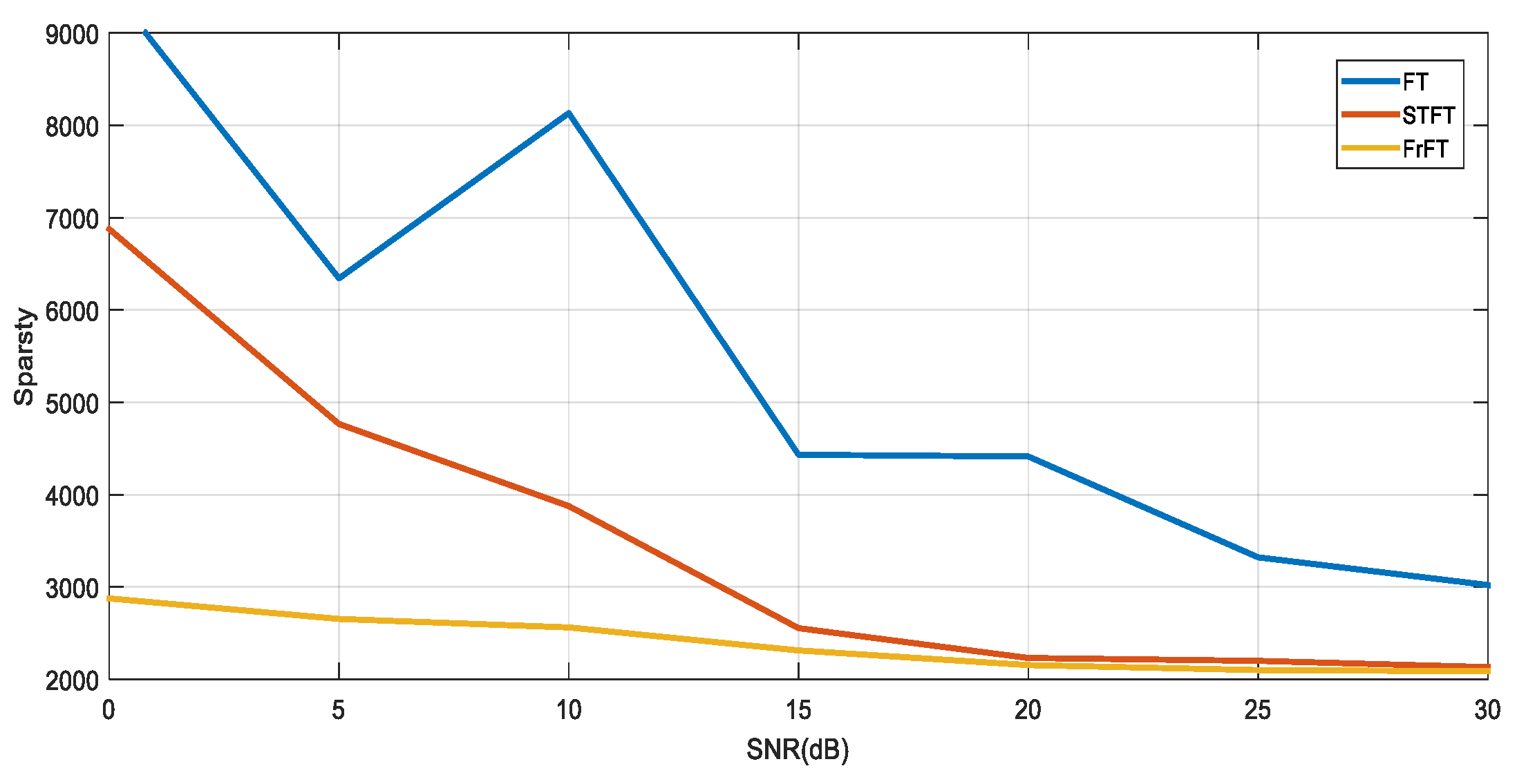
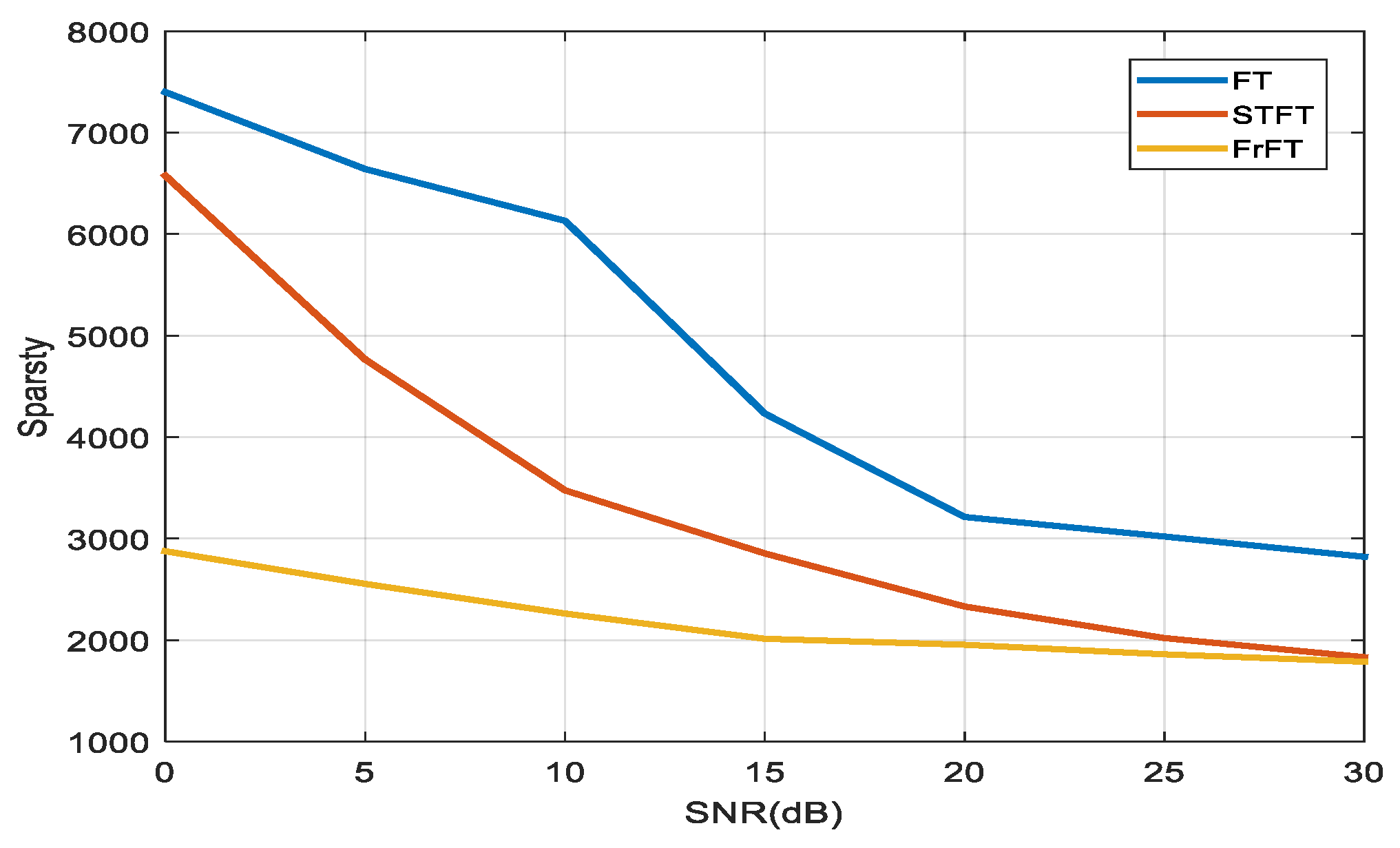
  34. Wang, S.; Guo, Y.; Yang, L. Research on FM signal sparsity in fractional Fourier transform domain. Optoelectron. Eng. 2020, 47, 190660. [Google Scholar]
Figure 1. Flow chart of α-UBSS algorithm proposed in this paper.
Electronics 12 00456 g001
Figure 2. Flow chart for searching α of FrFT.
Electronics 12 00456 g002
Figure 3. Noise suppression in fractional domain. (a) FrFT order search of pure signal; (b) FrFT order search of signal when SNR = 10 dB; (c) FrFT order search of signal when SNR = 5 dB; (d) FrFT order search of signal when SNR = 1 dB.
Electronics 12 00456 g003
Figure 4. Spectrum comparison of signals with different SNRs in the fractional domain of the same transformation order.
Electronics 12 00456 g004
Figure 5. Time domain waveform of six channel signals. ((af) is 6 different signals).
Electronics 12 00456 g005
Figure 6. Mixed signal after mixed matrix. (a) Time domain; (b) Frequency domain.
Electronics 12 00456 g006
Figure 7. Change of mixed-signal sparsity of the first receiving channel with order. (a,b) Rough search result; (c,d) Exact search result.
Electronics 12 00456 g007
Figure 8. Comparison of different domains of mixed signals in UBSS system. (a) time domain; (b) frequency domain; (c) time−frequency domain; (d) fractional domain under optimal transformation order p = −0.5194.
Electronics 12 00456 g008
Figure 9. Scatter plot comparison of mixed signals. (a) time domain; (b) frequency domain; (c) fractional domain proposed in [34]; (d) fractional domain proposed in our paper.
Electronics 12 00456 g009
Figure 10. Sparsity comparison at different SNRs after different transformations (single time).
Electronics 12 00456 g010
Figure 11. Sparsity comparison of different SNR after different transformations (50 times).
Electronics 12 00456 g011
Figure 12. Comparison of estimation accuracy of mixed matrix with different SNRs (single time).
Electronics 12 00456 g012
Figure 13. Comparison of estimation accuracy of mixed matrix with different SNRs (30 times).
Electronics 12 00456 g013
Figure 14. Comparison of the computational complexity of the algorithms proposed in [16,17] and this paper.
Electronics 12 00456 g014
Table 1. Research summary of the mixing matrix in recent years.
Ways of ImprovementPaperYearMethodNoveltyLimitation
Establishment of sparse model for observed signal[4]2007Directly complete the mixed matrix estimation in the time domainReduce the amount of computationNot valuable in engineering
applications
[5]2007Single Source Point (SSP)Increase the linear clustering characteristicsPseudo SSPs
[6]2013Improved SSP
detection
A singular value decomposition methodComputational load is greatly increased
[7]2018Local stationarity and distribution symmetry
[8]2019Low noise points
[9]2021lp (0 < p ≤ 1) regularisation to
reconstruct the sparse sources
Robustness to room reverberationComputational complexity
[10]2019Wavelet transformIncreases the time and frequency
information
Excessive redundancy
[11]2011Fractional Fourier
Transform (FrFT)
First proposed to use FrFT to implement BSSThe possibility is derived, but the actual algorithm is not given
[12]2014First proposed fractional time–frequency spaceSignal sparsity is not discussed
[13]2016Proposed using sparsity to study the fractional domainDiscussion on image signal only
[14]2017Using fractional field to realise FastICAOnly BSS is discussed
[15]2021Energy aggregation and insensitivityThe global threshold is used to search the fractional domain transformation order, which requires a large amount of computation
Selection of clustering methods[16]2017Hierarchical clusteringWithout setting initial valueHigh requirements on data
points
[17]2019Density-Based Spatial Clustering
of Applications with Noise (DBSCAN)
Automatically find the number of clusters
and the corresponding cluster centre
The number of clusters has a large error due to the presence of interference
[18]2019K-meansSimple and fastLocal optimal solution
[19]2019Particle Swarm Optimisation (PSO)Good determination of the number of
source signals
Unable to converge globally
[21]2020Directed Fuzzy C-Means (DFCM)Considers the directionInterfered with by outliers
Table 2. Six chirp signals with different parameters.
s i AmplitudeChirp RateStarting Frequency
s 1 1400200
s 2 5600400
s 3 10800400
s 4 10600200
s 5 10200100
s 6 15800600
Table 3. Comparison of estimation accuracy of mixed matrix obtained by different clustering algorithms.
Data SetNMSE
K-MeansDBSCAN
STFTFrFTSTFTFrFT
Clean signal −8.7679−14.1429−15.0967−18.4557
SNR = 0 −1.5434−8.4982−4.5434−10.9985
SNR = 5 −1.6442−9.2785−6.5421−12.4329
SNR = 10 −3.5643−9.5437−7.8739−13.3212
SNR = 15 −4.9838−10.2379−8.5470−15.4596
SNR = 20 −6.2324−11.9833−10.4534−16.6733
SNR = 25 −8.2294−13.7192−12.3858−17.8734
SNR = 30 −8.5430−14.0319−14.7854−18.3212
Table 4. Comparison of estimation accuracy of mixed matrix obtained by different clustering algorithms (30 times).
Data SetNMSE
K-MeansDBSCAN
STFTFrFTSTFTFrFT
Clean signal−9.0591−14.7524−15.1111−18.8518
SNR = 0−2.0793−8.1088−7.8875−11.3087
SNR = 5−3.7684−10.5634−8.6599−12.8743
SNR = 10−4.5609−11.5437−9.0765−13.7647
SNR = 15−6.3658−11.8675−10.8847−14.7824
SNR = 20−7.2324−12.6894−12.5973−16.2533
SNR = 25−8.2294−13.6219−13.5635−17.0053
SNR = 30−8.9430−14.4297−14.3764−18.4534
Disclaimer/Publisher’s Note: The statements, opinions and data contained in all publications are solely those of the individual author(s) and contributor(s) and not of MDPI and/or the editor(s). MDPI and/or the editor(s) disclaim responsibility for any injury to people or property resulting from any ideas, methods, instructions or products referred to in the content.

