Next Article in Journal
A Single-Coil Multi-Tapped PDM-Based Induction Heating System for Domestic Applications
Previous Article in Journal
Framework for Detecting Breast Cancer Risk Presence Using Deep Learning
 
 
Due to scheduled maintenance work on our database systems, there may be short service disruptions on this website between 10:00 and 11:00 CEST on June 14th.
Article

A Multidimensional Model for Recommendation Systems Based on Classification and Entropy

1
School of Computer Science (National Pilot Software Engineering School), Beijing University of Posts and Telecommunications, Beijing 100876, China
2
Key Laboratory of Trustworthy Distributed Computing and Service (BUPT), Ministry of Education, Beijing 100876, China
*
Author to whom correspondence should be addressed.
Electronics 2023, 12(2), 402; https://doi.org/10.3390/electronics12020402
Submission received: 6 December 2022 / Revised: 29 December 2022 / Accepted: 9 January 2023 / Published: 12 January 2023

Abstract

:
The proliferation of false and redundant information on e-commerce platforms as well as the prevalence of ineffective recommendations and other untrustworthy behaviors has seriously impeded the healthy development of these platforms. To address these issues and enhance prediction accuracy and user trust, contemporary recommendation systems often utilize additional information (i.e., side information). In this work, we propose a model to improve the recommendation quality by employing the information entropy of user-item ratings. The entropy was used as side information to reflect the global rating behavior of the user and item. We also utilized the classification of the user and item as heuristic information to improve the prediction quality. In our best result, we achieved a significant improvement of 8.2% in prediction accuracy. The model classified the items by the users’ actual preference, which is more trustworthy for users. We evaluated our model with three real-world datasets. The performance of our proposed model was significantly better than the other baseline methods. The similarity calculation method employed in the present model has the potential to mitigate the data sparsity problem associated with correlation-based similarity. The proposed weight matrix has zero sparsity. Furthermore, the proposed model has a more favorable computational complexity for prediction compared to the conventional k-nearest neighbor method.

1. Introduction

With the development of information technology and the growth of the Internet, users are continuously bombarded with an endless flood of information. As a result, people have many more options to choose from in every aspect of their lives, and the cost of obtaining accurate information also increases. Specifically, when there are more choices, it is much more difficult to find the information that best suits their needs and preferences [1,2]. The emergence of the recommendation system (RS) is mainly to solve the problem of information overload. The task of the recommendation system is to help users find information that is valuable to them [3]. These systems are now widely used to recommend different items such as goods, music, and movies. Using various data sources, it infers the interests and preferences of users [4]. For example, if a person reads a recommended article in a news aggregation app, the person will likely discover that it appeals to their interests. The recommendation engine calculates the individual’s preferences based on their past behavior, then selects the best news articles for them from many sources and presents them to the person.
Over the past few decades, the field of recommendation systems has seen significant advancements [5,6,7]. A variety of algorithms have been proposed and evaluated [8,9], which can be broadly classified into three categories: content-based, collaborative filtering (CF), and hybrid methods [10]. Content-based recommenders rely on extensive item descriptions (e.g., metadata, text descriptions, topics) to generate recommendations based on the feature vectors of the content. The effectiveness and accuracy of this type of recommendation system is directly correlated with the amount of information available about the user or item. For instance, content-based recommendation systems utilized by e-commerce platforms often utilize information such as product category, detailed product descriptions, price, and manufacturer [11,12,13]. However, this approach is prone to the “cold start” problem, whereby the system is unable to make recommendations for users or items with insufficient information, and is limited in its ability to explore the users’ potential interests [14,15]. Additionally, manual annotation is often required for media such as images and audio, which increases the workload for developers. CF, another widely used recommendation technique, involves analyzing the users’ historical feedback or behavior to identify patterns that can be used to predict the recommended items [16]. CF can be further divided into memory-based and model-based approaches. The underlying assumption of CF is that users with similar preferences will rate items similarly. This approach is commonly used by e-commerce companies to provide recommendations to customers [17,18,19]. However, CF suffers from the “cold start” problem [20] and has poor scalability, particularly when dealing with large datasets. Additionally, the “data sparsity” problem arises when a user has only rated a small number of items in the user-item matrix. Hybrid recommenders including weighted hybridization, switching hybridization, cascade hybridization, and mixed hybridization [21] are variations of content-based and CF methods. These approaches seek to combine the strengths of both methodologies in order to overcome their individual limitations.
In this paper, we focused on memory-based collaborative filtering [22]. The main challenge was to determine which group of users had a similar preference to the target users [16,23] (i.e., to find an appropriate measure of user similarity). Researchers have used different side-information [24,25,26,27] to obtain a more effective similarity to improve the prediction accuracy of recommendations [28,29]. It is natural to think that we are likely to accept suggestions from similar partners [30,31]. For this reason, many aspects of both users and items are often used as auxiliary information to find similar preferences among users in CF [17,18,19,20,21]. However, due to various reasons, it is difficult to obtain a direct similarity relationship. In contrast, implicit similarity relationships are inferred from user preferences. If a user is more knowledgeable about a given subject, we assume that they are more reliable. Information entropy is the indicator that we can use to measure the amount of information [32,33]. This is a popular indicator to measure the amount of useful information and is often used by researchers to improve accuracy [21,34,35]. By using information entropy of the ratings on items and users, our proposed method considers the rating behavior of users on each common item as well as the history of ratings made by each user. We then used the entropy to make a rating prediction. Inspired by the traditional kNN method [36,37], we proposed a novel method of choosing neighbors. We then merged the entropy with classification information. We used classification information to find a more suitable similar user in the global view.
This study proposed a recommendation system that utilizes entropy and classification information to generate personalized product recommendations based on user evaluations. The proposed multidimensional model, referred to as UITrust, enables the recommendation system to identify trustworthy and similar users. Unlike traditional similarity matrices, the proposed similarity matrix did not contain empty entries. Through the use of the proposed method, we observed significant improvements in comparison to other baseline methods across three real-world datasets. The specific contributions of this research include the following:
  • We propose a new multidimensional recommender model called UITrust that utilizes classification information and entropy to improve the prediction accuracy.
  • Reduce both the computational complexity of prediction and the sparsity of the weight matrix compared with the baseline methods.
  • Using three real-world datasets and the experimental results, we show that the proposed model is superior to other benchmark methods including traditional kNN-based methods.
  • Proposed a novel approach for explainability in the recommender.
The present study presents a framework that can be effectively implemented in online e-commerce systems to assist sellers in promoting their products and services.
The subsequent section formally defines the problem and presents the proposed model. Subsequently, we outline the experimental environment and provide a comparison of the evaluation results of the proposed model with a baseline. The final section concludes the article by briefly discussing the limitations of the proposed method and suggesting avenues for future research.

2. Proposed Model

2.1. Preliminaries

Memory-based CF methods have been adopted in different practical industrial systems because of their simplicity and effectiveness. These approaches generally use the ratings vector to indicate user preference. The rating history is used to find similar users/items, also called neighbors. These can be identified by a similarity measure that represents the differentiation between two users. With the selected neighbors, the ratings to be predicted are calculated by aggregating the ratings of neighbors. We model the prediction process as follows.

2.2. Model

The objective of this study was to predict ratings for items that have not yet been rated by a user, based on the user’s rating history data. A common approach to achieve this is to calculate the similarity between the target user and a set of k neighbors, and to weight the ratings of these neighbors accordingly. As a baseline, we utilized the basic k-nearest neighbor (kNN) formula outlined below.
r u , i ^ = v N i   k u S i m u , v × r v , i v N i   k u S i m u , v ,
where r u , i ,   r v , i     R U × I is the ratings of users u ,   v     U for item i     I in the rating matrix R U × I . In this equation, r u , i ^ is the prediction of item i for user u . N i   k u is the set of k neighbors of user u who have rated the item i , r v , i is the rating given to item i by the neighbor v , and S i m u , v is the similarity between user u and user v . The similarity between u and v is calculated using the Pearson correlation, which is given by:
S i m u , v = i I u I v r u , i r u , i ¯ r v , i r v , i ¯ i I u I v r u , i r u , i ¯ 2 i I u I v r v , i r v , i ¯ 2 ,
where r u , i ¯ and r v , i ¯ are the average rating of the respective user. In Equation (2), based on the correlation of user u , v ’s commonly rated items, we can obtain the similarity between any two users. The most essential work for memory-based CF is the identification of neighbors and the rating prediction. In the following section, we propose two novel measures for these two points.

2.2.1. Classification-Based k-Neighbor Selection Measure

When trying to calculate the similarity of two users, in general, conventional similarity is the distance between two vectors. The size of the similarity matrix will be either the number of users by number of items in the dataset. The measure only focuses on the common item’s rating vector. However, in the case where two users have no common rating, their similarity will be zero. Here, we intend to use the classification of the item along with the taste of each user. In this way, every user for every item will have a value.
We focused on using item classifications, specifically movie genres, to pick the neighbors. We derived the user’s taste for an item using the ratings expressed. Similarly, using the collective ratings given to an item, we identified how much each item belongs to a certain genre. These two vectors are then combined to obtain a user–item–weight matrix. In contrast to the similarity-based weight matrix in memory-based collaborative filtering, we used the user–item–weight to rank the prediction contributor candidate so that we could have the most similar neighbor, and at the same time, we can assume that this neighbor is also familiar with the type of item, implying that this user’s suggestion is valuable.
Let G = g 1 , g 2 ,   , g k ,   , g m be aa set of all classifications of the items in the dataset. Item i I can be represented in terms of a vector of classifications g i as in the following equation.
g i = g i 1 , g i 2 ,   , g i k , , g i m ,
The g i k will be 1 if item i is labeled classification g k . If not, the value of g i k will be zero. For example, the dataset has three genres, horror, comedy, and romance, and G maintains that order. If movie X is a romantic comedy, then it is labeled as both comedy and romance. Therefore, movie X’s classification vector g i   will   be   0 , 1 , 1 . Since all movies are labeled with one or more genres by the producers, a movie always has at least one classification (i.e., g i k = 1 > 0 ). For all items i I u rated by user u , and if the classification g i k = 1 , then g i k = r u i , composing a new vector g i * from g i . Therefore, continuing with the example of movie X with user u, if the rated movie X has three stars, then g x * will be {0,3,3}. The user-classification vector of user u can be calculated as follows:
s u , k = i I u g i , k * i I u g i * ,
where s u , k indicates the user-classification for the kth genre and the denominator is the sum of the total ratings in g i * . The denominator can also be interpreted as the total collective ratings given to all genres by user u . Please note that this value is always greater than or equal to the user u ’s total rating. The value of each entry in the resulting vector s u , k   represents user u ’s degree of preference for the genre k . For a worked example, consider a horror movie Y to which the user rates five stars, thus g y * = {5,0,0}. The s u , k will be 5/11 = 0.45, where k is the index of the horror genre. One of the advantages of this metric is that it defines the user’s preference for a specific genre as a continuous value rather than a discrete value. The full s u vector will be {0.45, 0.27, 0.27}.
As mentioned earlier, movies are classified by producers or experts. However, this classification does not consider the viewers’ opinions. Initially, we represented this as a binary vector g i in Equation (4). Since collaborative filtering uses other users’ views while making predictions, it is intuitive that the movie recommendation using genre information in the process would increase the prediction accuracy. Additionally, it is intuitive to consider all of the user’s ratings (i.e., users’ preferences) to estimate the actual genres of the movies, rather than simply relying on the producers or experts. Let S be the set containing all of the user-classifications s u   . The shape of S would be U × g . We calculated the new genre values c i for movies as follows:
c i = u U i s u × r u , i v U s v × r v , i ,
where r u , i , r v , j     R U × I is the rating by the user u U i , who has rated item i and s u ,   s u   S , whereas v is from the set of all user U who rated item j in the dataset. Here in the numerator of the equation, the user-classification s u is multiplied by the user’s rating. Similar to the elements of s u , elements of c i range between zero and one. Let us assume there is a second user z who only rated the movie Y with three starts. Now, the s u and s z are {0.35, 0.21, 0.21} and {0.57, 0.0, 0.0}. The new genre value calculated using Equation (5) for the item Y will be ({0.35, 0.21, 0.21} × 5)/({0.35, 0.21, 0.21} × 5 + {0.57, 0.0, 0.0} × 4) = {0.75, 1, 1}. The final user–item–weight score is calculated by taking the dot product of both the user’s taste s u and c i as follows:
w u , i = s u   c i ,
where w u , i is the user–item weight. Then, we used the w u , i to sort the pending items in the dataset. The final weight w u , i for user u for the item i was {0.73, 1, 1} {0.35,0.21,0.21} = 0.699. Since every item and user pair has a weight value, the shape of the user–item matrix will be the number of users by the number of items in the dataset. For the item-based methods, we can simply transpose the matrix.

2.2.2. Entropy-Driven User–Item Similarity

In traditional CF, the similarity between users, which serves as a weight matrix, is just one of the most important factors that affect the accuracy of the prediction. Several possible factors can be used to improve the prediction accuracy or even enhance the system’s performance.
The whole calculation process of calculating the final weight matrix is shown in Figure 1:
We formulated the similarity measure, which can obtain the information from entropy for each prediction. In Equation (7), we defined the p r o b _ I i r , the probability p r o b r i = r of rating r the item i . The numerator of the equation indicates the number of ratings that is equal to the currently calibrated value. The denominator is the total number of ratings obtained from this item. Here, our model used this variable to indicate the probability of each possible rating. We can apply the same idea for the user, as shown in Equation (8).
p r o b _ I i r = u U   r u , i = r u U   r u , i r min , r max ,
p r o b _ U u r = i I   r u , i = r i I r u , i r min , r max ,
By studying p r o b _ I i r and p r o b _ U u r , the frequency at which the current rating occurs among the user’s historical ratings, we can determine the information content of the rating. Considering the example users, items, and ratings from the previous subsection and applying Equation (7), the probability p r o b _ I y 3 of item Y rated with three stars was 1/2. Similarly applying Equation (8), the probability p r o b _ U u 5 of user u rating an item with five stars was 1/2. Next, we incorporated the concept of entropy into the model to help it make better predictions. We assumed that the trust could be increased by adding more information to the system. Therefore, we can use the combined entropy of the user and item. As a result, we can choose the ones that have the most information, providing a more trustworthy recommendation for users. As seen in the following equation, we simply used H i to indicate the degree to which the content of the message is more surprising. The higher value of H i means that the information contained in the log values of the item/user is higher, making the final prediction better. Here, we used the entropy calculation method for items and users separately, then we can obtain H o I i and H o U u , which indicate the entropy of the item and the entropy of the user. With the higher H o l i \ H o U u , we can learn which item/user’s vector contains more information. The formulas are shown below:
H o I i = r = r m i n r m a x p r o b _ I i r log 2 p r o b _ I i r ,
H o U u = r = r m i n r m a x p r o b _ U u r log 2 p r o b _ U U r ,
In order to make predictions, we used a new similarity to use as weights in this process. We combined the user–item weight w u , i mentioned in the last section and the average of the H o l i and H o U u , which is denoted as U I T r u s t . The formula is shown below:
U I T r u s t u , v = α w u , i + 1 α Hol i +   HoU u 2  
where α is the hyperparameter in the formula. Consider the extreme case where only one item i has been rated with a single star by a single user and no other user have rated that item. The p r o b _ I i 1 will be 1 and H o I i will be zero. Similarly the H o U u can also be zero. However, as long as α is not equal to 1 in Equation (11), there will always be a U I T r u s t value. We used this new similarity U I T r u s t u , v , which uses information entropy and classification information, to calculate the final prediction. The final prediction r u , i ^ is made by using the mean rating r u ¯ of the target user u , adding the bias part to it as follows:
r u , i ^ = r u ¯ + j N k u U I T r u s t u , v × r u , j j N k u U I T r u s t u , v ,
where N k u is the set of neighbors selected by the weighted sum of classification-based k -neighbor selection measure. With the help of the information entropy, we can now effectively incorporate the contribution of neighbors, reflecting the global rating behavior on the user and item rating history.

3. Results and Evaluation

3.1. Evaluation Indicators

The quality of the recommendation algorithm is determined using evaluation metrics that often provide different perspectives. They are widely used in both research and practice. One of the most common evaluation metrics used for prediction accuracy is the mean absolute error (MAE) [38,39]. The MAE measures the absolute difference between the actual value and predicted values as an error, which is given by:
M A E = 1 R ^ r u , i ^ R ^ r u , i r u , i ^ ,
where R ^ is the set of predictions.
In contrast to taking absolute values, RMSE squares the error and takes the square root to deal with the negative values. RMSE also punishes larger errors heavily. RMSE is calculated as follows:
  R M S E = 1   R ^ r u , i ^ R ^ r u , i r u , i ^ 2 ,

3.2. Dataset

In this paper, three different public benchmark datasets from MovieLens (GroupLens, University of Minnesota, Minneapolis, MN, USA) were used to evaluate the proposed algorithm [40]: (1) ML-100k; (2) ML-latest-small; and (3) ML-1m. To better illustrate the validity of the algorithm, we defined density to describe the sparsity for each dataset, which is calculated as follows:
D e n s i t y = R U × I ,
where R refers to the number of ratings in the dataset. The details about these three datasets are provided as follows:
  • The MovieLens 100K dataset was collected by the GroupLens Research Project at the University of Minnesota. This dataset consists of 100,000 ratings from 943 users on 1682 movies;
  • The ML-latest-small dataset, the same as the first one, was also collected by the same project. It contains 100,836 ratings and 3683 tag applications across 9742 movies. The rating scale is 0.5 to 5;
  • The MovieLens 1M dataset contains 1,000,209 anonymous ratings of 3900 movies made by 6040 MovieLens users who joined MovieLens in 2000.
Additional details about the datasets are provided in Table 1.
From the results, we can see that these datasets were not dense. Therefore, it was necessary to find some measures to overcome the problems caused by data sparsity. To ensure the validity of the algorithm, we divided each dataset into two parts: 80% of the data was used as the training set, and the remaining 20% was used as the test set.

3.3. Experimental Setup

In this study, we utilized the Surprise framework, a python-based library widely utilized by both researchers and practitioners, to implement our algorithm. The Surprise framework, developed by Hug et al. [41], is highly modular and features several benchmark recommendation algorithms. Due to the high memory requirements of memory-based collaborative filtering (CF) methods, which store the weight matrix in memory, we conducted our experiments on a Dell PowerEdge T630 server equipped with 2.1 Hz 32 cores and 64 GB of RAM. The data for our experiments were structured as tuples comprising the user ID, item ID, ratings, and timestamps. We employed five-fold cross-validation for all datasets and test methods and compared our results to several existing approaches:
  • UITrust_C: Our proposed method, as in Equation (11), with k neighbor was chosen using the classification-based k-neighbor selection measure;
  • UITrust_P: Our proposed method, as in Equation (11), with k-neighbor was chosen using the Pearson similarity;
  • UITrust_MSD: Our proposed method, as in Equation (11), with k -neighbor was chosen using MSD similarity;
  • UITrust_R: Our proposed method, as in Equation (11), with k -neighbor was chosen by Random;
  • CKNN_P: A basic collaborative filtering algorithm, taking into account the mean ratings of each user, with k -neighbor chosen using Pearson similarity;
  • CKNN_MSD: A basic collaborative filtering algorithm, taking into account the mean ratings of each user, with k -neighbor chosen using MSD similarity;
  • BKNN_P: A basic collaborative filtering algorithm with k -neighbor was chosen using Pearson similarity;
  • BKNN_MSD: A basic collaborative filtering algorithm with k -neighbor was chosen using MSD similarity.

3.4. Experimental Results

3.4.1. Results on the ML-100k Dataset

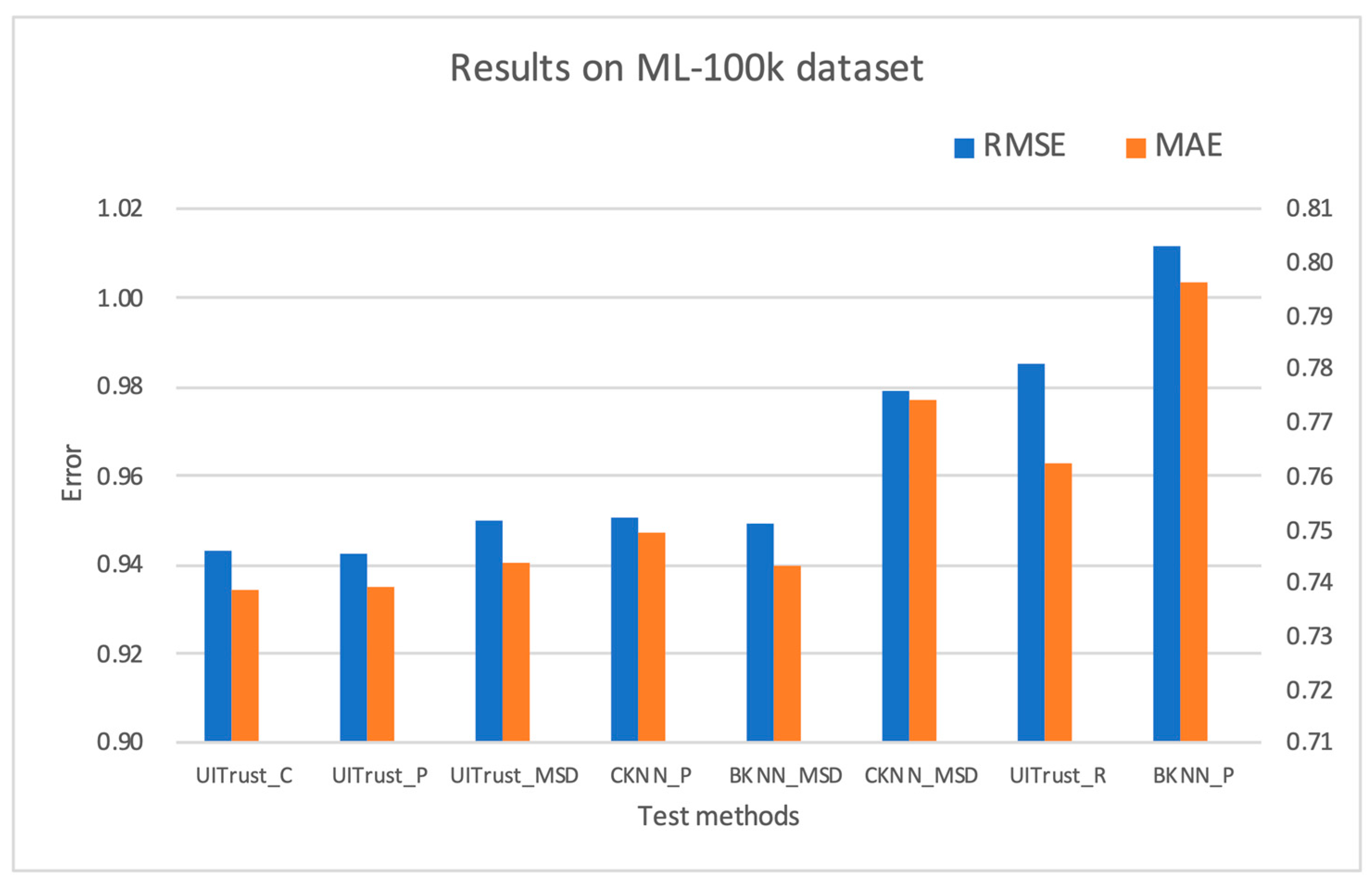
Figure 2 illustrates the prediction accuracy results obtained on the ML-100k dataset for the various methods being studied.
As shown in Figure 2, the results indicate that the proposed method (UITrust_C) using a classification-based measure as the neighbor selection method performed the best on the 100k dataset, with a slight increase in the mean absolute error (MAE) of 0.03% compared to UITrust_P, and a slight increase in the root mean squared error (RMSE) and MAE of 0.63% and 0.59%, respectively, compared to CKNN_P (using the same neighbor selection method). In comparison to CKNN_MSD, UITrust_C showed a more significant increase in accuracy, with an increase of 1.38% in MAE. In addition, UITrust_C exhibited a significant improvement against BKNN_P, with an increase of 6.80% in RMSE and 7.21% in MAE. There was also a significant improvement against BKNN_MSD, with an increase of 3.6% in RMSE and 4.53% in MAE.
The performance of UITrust_P was similar to that of UITrust_C. However, UITrust_MSD did not show any advantage compared to CKNN_P, but exhibited an improvement of 0.07% in RMSE and 0.74% in MAE compared to CKNN_MSD, and an improvement of 6.12% in RMSE and 6.62% in MAE compared to BKNN_P as well as an improvement of 2.94% in RMSE and 3.92% in MAE compared to BKNN_MSD. As for UITrust_R, the method did not perform better than CKNN_P, CKNN_MSD, and BKNN_MSD, but still showed improvements of 2.62% in RMSE and 4.28% in MAE compared to BKNN_P.

3.4.2. Results on the ML-Latest-Small Dataset

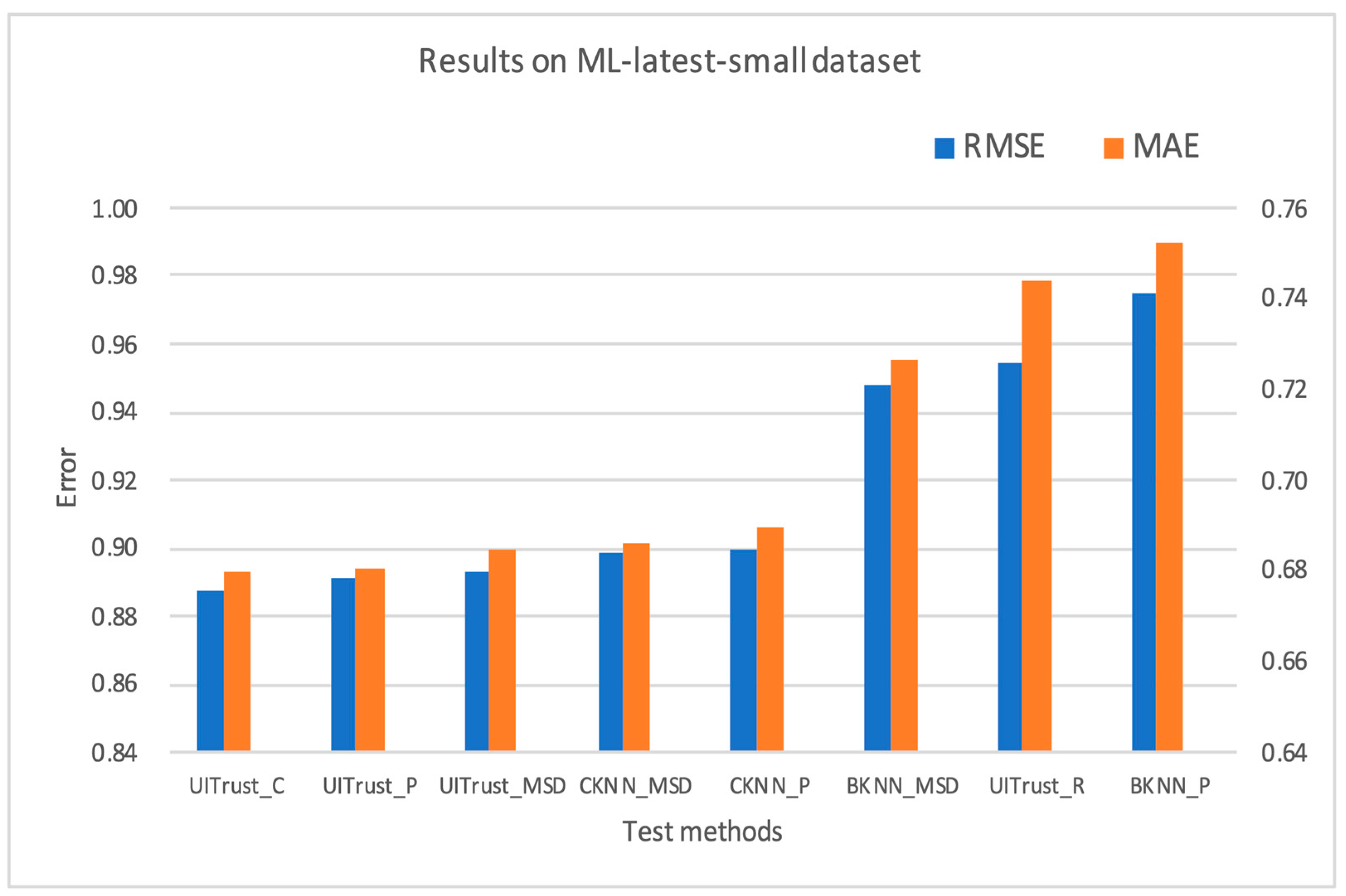
Figure 3 illustrates the prediction accuracy results obtained for the ML-latest-small dataset for the different methods being studied.
The results for the ML-latest-small dataset showed a similar pattern to those obtained on the ML-100k dataset as shown in Figure 3. In particular, UITrust_C ranked first, with a slight increase of 0.55% in the root mean squared error (RMSE) and 0.12% in the mean absolute error (MAE) compared to UITrust_MSD. There was also an increase of 1.16% in RMSE and 0.92% in MAE compared to the official baseline method CKNN_MSD. In addition, we found that UITrust with the mean squared difference (MSD) similarity exhibited a significant improvement against BKNN_MSD, with an increase of 5.81% in RMSE and 6.30% in MAE. Similarly, UITrust_P with the Pearson similarity showed a significant improvement against BKNN_P, with an increase of 8.62% in RMSE and 8.41% in MAE. Both UITrust_P and UITrust_MSD performed roughly as well as the method using entropy-based similarity. However, UITrust_P did not outperform the CKNN methods in terms of MAE. As for UITrust_R, this method did not perform better than CKNN_P, CKNN_MSD, and BKNN_MSD, but still exhibited an increase of 2.13% in RMSE and 1.18% in MAE compared to BKNN_P.
It is important to note that this dataset had the lowest density (i.e., the highest sparsity). Since both ML-100K and ML-latest-small had roughly the same number of ratings and significant improvements in UITrust-based methods compared to the baselines, it is clear that there is a significant contribution to improvements in prediction accuracy due to improved sparsity in our weight matrix.

3.4.3. Results on the ML-1m Dataset

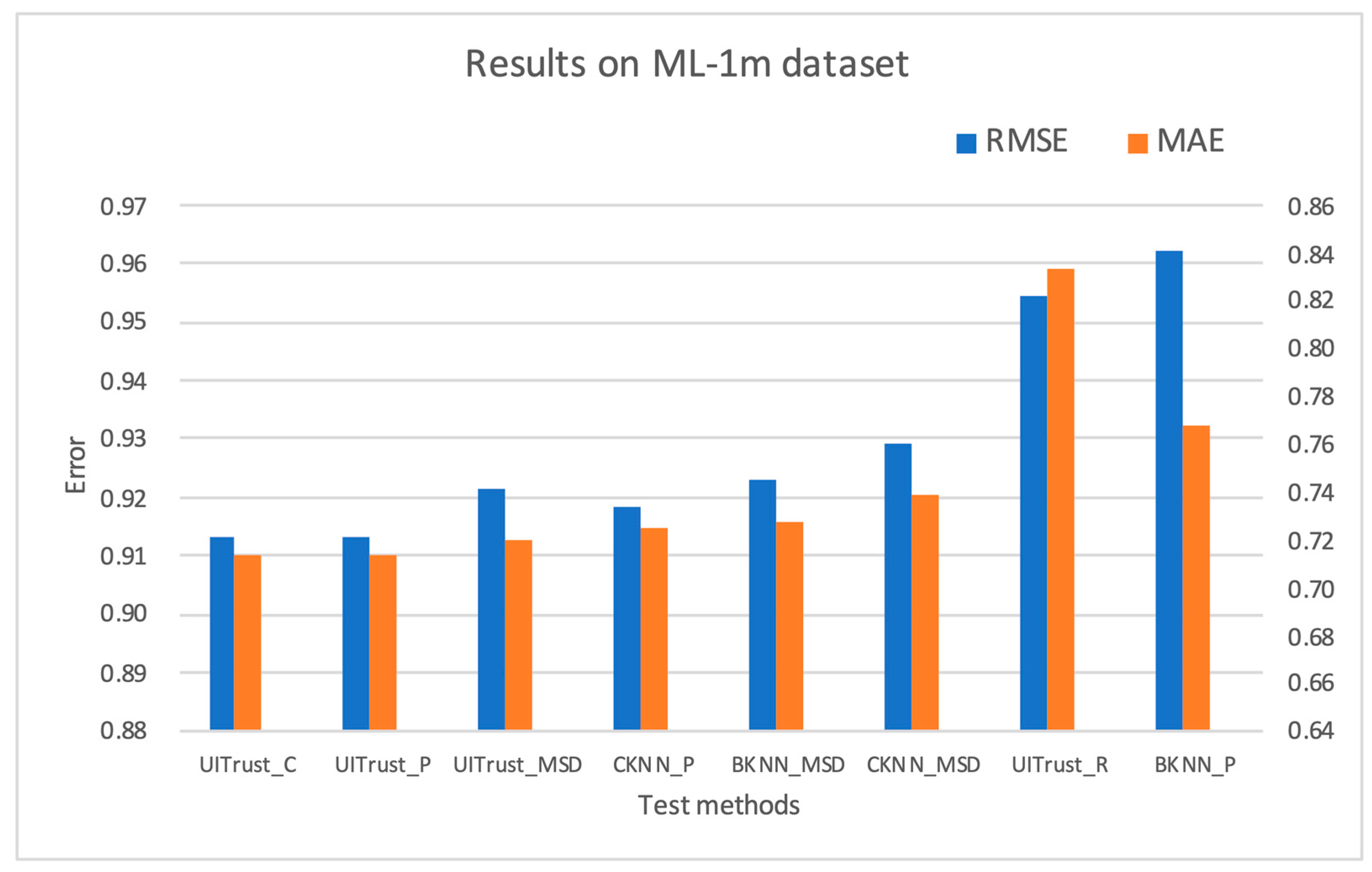
Figure 4 illustrates the prediction accuracy results obtained for the ML-1m dataset for the different methods being studied.
The prediction accuracy of the current dataset was found to be superior to that of the other two datasets. As the size of the dataset increased, the effectiveness of our approach became more pronounced. The performance of UITrust_C and UITrust_P was almost identical, as shown in Figure 4. UITrust_C exhibited an increase of 0.56% in the root mean squared error (RMSE) and 1.49% in the mean absolute error (MAE) compared to CKNN_P, and a more significant increase of 5.07% in RMSE and 6.70% in MAE compared to BKNN_P. There was also an improvement of 1.72% in RMSE and 3.34% in MAE compared to BKNN_MSD.
Similarly, UITrust_P showed an improvement of 1.70% in RMSE and 3.34% in MAE compared to CKNN_MSD, and a significant improvement of 5.06% in RMSE and 6.99% in MAE compared to BKNN_P.

3.4.4. Sparsity of Weight Matrix

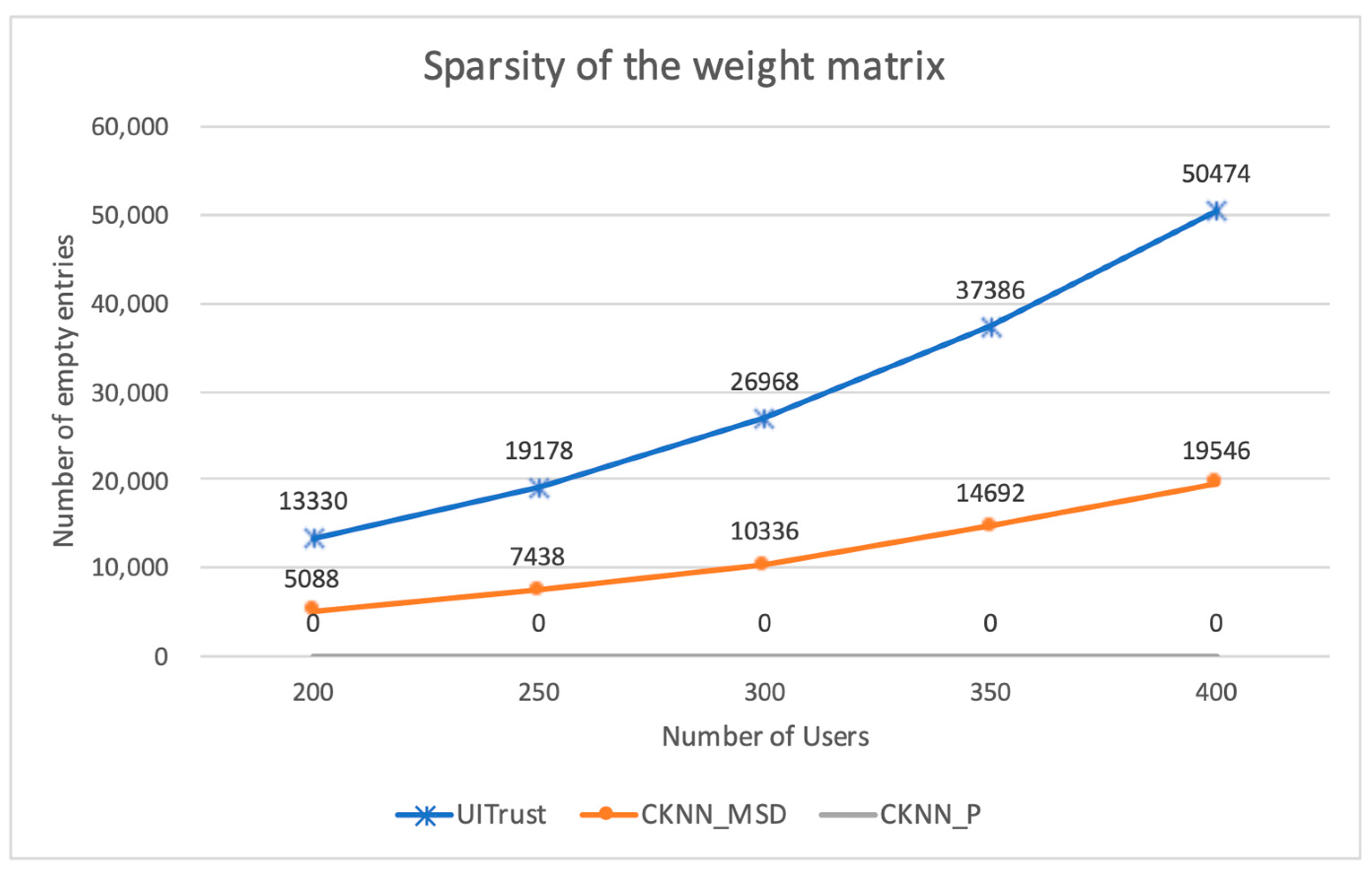
In order to compare the sparsity of the weight matrices among different methods, in Figure 5, we present a plot showing the number of empty entries in the weight matrix. The dataset that we used here was ML-100k. For the kNN-based methods, the weight matrix was the similarity matrix. We chose two different types of similarities, MSD and Pearson, for the result comparison. For our method, we used the classification-based k-neighbor selection measure and entropy-driven user–item similarity for plotting.
As seen in Figure 5, the increase in the number of users increased the sparsity of the weight matrices for the MSD and Pearson similarity. The average rate in the increase in the sparseness of the Pearson similarity matrix was roughly 2.5 times that of the MSD similarity matrix. However, for UITrust, regardless of the classification-based k-neighbor selection measure or other measures such as Pearson or MSD, the plot of them showed a flat zero, meaning that one of the users for all items always has a weight value. As discussed earlier, decreasing the sparsity is important as it impacts the accuracy of the predictions and our proposed method addressed this issue.

4. Discussion

The proposed method had significantly better prediction accuracy compared with other traditional kNN-based methods. Traditional methods of calculating similarity include MSD similarity and the Pearson correlation method. The Pearson correlation coefficient is based on the premise that both users must rate the same items and helps to choose similar users. As for MSD, only the number of items rated jointly by users is considered, but the rating of the same item between users is not considered. None of these methods solved the problem of data sparsity in the user–item matrix. One of the advantages of our proposed method is that we can have a distinct prediction result for users who have no neighbors. The classification-based k-neighbor selection measure helps significantly improve the result’s coverage and well addresses the data sparsity issue. Additionally, during the pre-computation process, our method considers the multi-dimensional information input, so we can have a reasonable graph of the calculations and results. It proposes a novel approach for interpretability in a recommender. Compared with the correlation-based similarity, the utilization of entropy also helps our proposed method reflect the global rating behaviors of users and items. Therefore, we can take into account the analysis of the overall dataset while taking into account the influence of the neighbors of the users.
However, the disadvantages are also obvious. In real-time situations, the recommendation system has no conditions to calculate the overall fluctuation of the data in real-time. Therefore, we cannot have the entropy value at a negligible length of time. This method will reduce the recommendation efficiency in this situation. At the same time, this method is not suitable for interactive recommendation systems. Our proposed measure will be more suitable for small-scaled sparse datasets.

5. Conclusions

In this study, we proposed a recommendation system algorithm that incorporates information entropy and classification information to improve the prediction accuracy. To evaluate the efficacy of our approach, we conducted experiments on three real-world datasets. The key concept behind our algorithm is the utilization of entropy in ratings for each user and item to capture the variability within the datasets, which is then integrated into traditional similarity measures in order to identify contributors with the highest amount of information, and thus the greatest level of trustworthiness. These contributors were also identified through a classification-based k-neighbor selection process, ensuring that they were familiar with the specific item being recommended. This led to more trustworthy recommendations and improved coverage compared to kNN-based methods due to the reduced sparsity of the new similarity measure. Furthermore, our method provides explainable recommendations, providing users with multiple dimensions of information to personalize the recommendation process and enhance the prediction performance. Our experiments on the MovieLens datasets demonstrate the ability of our method to enhance the prediction quality. In future work, we plan to further examine the performance of our method on modern and dense datasets from various domains, and to address the issue of a small, static dataset size in order to apply our approach to interactive industrial environments. We also intend to assess the performance of our method using various metrics such as reliability and diversity through additional experiments. It is important to note the gain in popularity of deep learning technologies in recommendation research, and in future work, we plan to compare and incorporate our method with modern deep learning approaches.

Author Contributions

Conceptualization, Y.Y., L.C. and J.Y.; Formal analysis, L.C.; Investigation, Y.Y. and L.C.; Methodology, L.C. and Y.Y.; Project administration, Y.Y.; Resources, L.C.; Software, L.C.; Supervision, J.Y.; Validation, L.C., Y.Y. and J.Y.; Visualization, L.C. and J.Y.; Writing—original draft preparation, L.C.; Writing—review and editing, Y.Y. and L.C. All authors have read and agreed to the published version of the manuscript.

Funding

This research was supported by the National Natural Science Foundation of China (No. 91118002).

Institutional Review Board Statement

Not applicable.

Informed Consent Statement

Not applicable.

Data Availability Statement

For reproducibility, the data can be found at https://grouplens.org/datasets/movielens/ (accessed on 9 January 2023).

Conflicts of Interest

The authors declare no conflict of interest.

References

  1. Gomez-Uribe, C.A.; Hunt, N. The Netflix Recommender System: Algorithms, Business Value, and Innovation. ACM Trans. Manag. Inf. Syst. 2016, 6, 13. [Google Scholar] [CrossRef] [Green Version]
  2. Wang, S.; Zhang, X.; Wang, Y.; Liu, H.; Ricci, F. Trustworthy Recommender Systems. arXiv 2022, arXiv:2208.06265. [Google Scholar]
  3. Burke, R. Hybrid Recommender Systems: Survey and Experiments. User Model. User-Adap. Inter. 2002, 12, 331–370. [Google Scholar] [CrossRef]
  4. Mansur, F.; Patel, V.; Patel, M. A Review on Recommender Systems. In Proceedings of the 2017 International Conference on Innovations in Information, Embedded and Communication Systems (ICIIECS), Coimbatore, India, 17–18 March 2017; pp. 1–6. [Google Scholar]
  5. Koren, Y.; Rendle, S.; Bell, R. Advances in Collaborative Filtering. In Recommender Systems Handbook; Springer: Boston, MA, USA, 2022; pp. 91–142. [Google Scholar] [CrossRef]
  6. Ko, H.; Lee, S.; Park, Y.; Choi, A. A Survey of Recommendation Systems: Recommendation Models, Techniques, and Application Fields. Electronics 2022, 11, 141. [Google Scholar] [CrossRef]
  7. Dhelim, S.; Aung, N.; Bouras, M.A.; Ning, H.; Cambria, E. A Survey on Personality-Aware Recommendation Systems. Artif. Intell. Rev. 2022, 55, 2409–2454. [Google Scholar] [CrossRef]
  8. Meo, P.D. Trust Prediction via Matrix Factorisation. ACM Trans. Internet Technol. 2019, 19, 44. [Google Scholar] [CrossRef]
  9. Zhao, J.; Wang, W.; Zhang, Z.; Sun, Q.; Huo, H.; Qu, L.; Zheng, S. TrustTF: A Tensor Factorization Model Using User Trust and Implicit Feedback for Context-Aware Recommender Systems. Knowl.-Based Syst. 2020, 209, 106434. [Google Scholar] [CrossRef]
  10. Ricci, F.; Rokach, L.; Shapira, B.; Kantor, P.B. (Eds.) Recommender Systems Handbook; Springer: Boston, MA, USA, 2011; ISBN 978-0-387-85819-7. [Google Scholar]
  11. Schafer, J.B.; Konstan, J.A.; Riedl, J. E-Commerce Recommendation Applications. Data Min. Knowl. Discov. 2001, 5, 115–153. [Google Scholar] [CrossRef]
  12. Li, S.S.; Karahanna, E. Online Recommendation Systems in a B2C E-Commerce Context: A Review and Future Directions. J. Assoc. Inf. Syst. 2015, 16, 72–107. [Google Scholar] [CrossRef] [Green Version]
  13. Hussien, F.T.A.; Rahma, A.M.S.; Wahab, H.B.A. Recommendation Systems For E-Commerce Systems An Overview. J. Phys. Conf. Ser. 2021, 1897, 012024. [Google Scholar] [CrossRef]
  14. Zhang, Z.; Liu, Y.; Jin, Z.; Zhang, R. Selecting Influential and Trustworthy Neighbors for Collaborative Filtering Recommender Systems. In Proceedings of the 2017 IEEE 7th Annual Computing and Communication Workshop and Conference (CCWC), Las Vegas, NV, USA, 9–11 January 2017; pp. 1–7. [Google Scholar]
  15. Celikik, M.; Wasilewski, J.; Mbarek, S.; Celayes, P.; Gagliardi, P.; Pham, D.; Karessli, N.; Ramallo, A.P. Reusable Self-Attention-Based Recommender System for Fashion. arXiv 2022, arXiv:2211.16366. [Google Scholar]
  16. Jiang, L.; Cheng, Y.; Yang, L.; Li, J.; Yan, H.; Wang, X. A Trust-Based Collaborative Filtering Algorithm for E-Commerce Recommendation System. J. Ambient Intell. Human. Comput. 2019, 10, 3023–3034. [Google Scholar] [CrossRef] [Green Version]
  17. Kadek Abi Satria, A.V.P.; Baizal, Z.K.A. Improved Collaborative Filtering Recommender System Based on Missing Values Imputation on E-Commerce. Build. Inform. Technol. Sci. 2022, 3, 453–459. [Google Scholar] [CrossRef]
  18. Liao, M.; Sundar, S.S. When E-Commerce Personalization Systems Show and Tell: Investigating the Relative Persuasive Appeal of Content-Based versus Collaborative Filtering. J. Advert. 2022, 51, 256–267. [Google Scholar] [CrossRef]
  19. Khatter, H.; Arif, S.; Singh, U.; Mathur, S.; Jain, S. Product Recommendation System for E-Commerce Using Collaborative Filtering and Textual Clustering. In Proceedings of the 2021 Third International Conference on Inventive Research in Computing Applications (ICIRCA), Coimbatore, India, 2–4 September 2021; pp. 612–618. [Google Scholar]
  20. Mnih, A.; Salakhutdinov, R.R. Probabilistic Matrix Factorization. In Advances in Neural Information Processing Systems; Curran Associates, Inc.: New York, NY, USA, 2007; Volume 20. [Google Scholar]
  21. Lee, S. Using Entropy for Similarity Measures in Collaborative Filtering. J. Ambient Intell. Human. Comput. 2020, 11, 363–374. [Google Scholar] [CrossRef]
  22. Pirasteh, P.; Bouguelia, M.-R.; Santosh, K.C. Personalized Recommendation: An Enhanced Hybrid Collaborative Filtering. Adv. Comp. Int. 2021, 1, 1. [Google Scholar] [CrossRef]
  23. Guo, G.; Zhang, J.; Thalmann, D. Merging Trust in Collaborative Filtering to Alleviate Data Sparsity and Cold Start. Knowl.-Based Syst. 2014, 57, 57–68. [Google Scholar] [CrossRef]
  24. Niu, J.; Wang, L.; Liu, X.; Yu, S. FUIR: Fusing User and Item Information to Deal with Data Sparsity by Using Side Information in Recommendation Systems. J. Netw. Comput. Appl. 2016, 70, 41–50. [Google Scholar] [CrossRef]
  25. Ning, X.; Karypis, G. Sparse Linear Methods with Side Information for Top-n Recommendations. In Proceedings of the Sixth ACM Conference on Recommender Systems, Dublin, Ireland, 9–13 September 2012; Association for Computing Machinery: New York, NY, USA, 2012; pp. 155–162. [Google Scholar]
  26. Rafailidis, D.; Nanopoulos, A. Modeling Users Preference Dynamics and Side Information in Recommender Systems. IEEE Trans. Syst. Man Cybern. Syst. 2016, 46, 782–792. [Google Scholar] [CrossRef]
  27. Liu, T.; Wang, Z.; Tang, J.; Yang, S.; Huang, G.Y.; Liu, Z. Recommender Systems with Heterogeneous Side Information. arXiv 2019, arXiv:1907.08679. [Google Scholar]
  28. Chen, L.; Yuan, Y.; Jiang, H.; Guo, T.; Zhao, P.; Shi, J. A Novel Trust-Based Model for Collaborative Filtering Recommendation Systems Using Entropy. In Proceedings of the 2021 8th International Conference on Dependable Systems and Their Applications (DSA), Yinchuan, China, 5–6 August 2021; pp. 184–188. [Google Scholar]
  29. Chen, L.; Yuan, Y.; Yang, J.; Zahir, A. Improving the Prediction Quality in Memory-Based Collaborative Filtering Using Categorical Features. Electronics 2021, 10, 214. [Google Scholar] [CrossRef]
  30. Zahir, A.; Yuan, Y.; Moniz, K. AgreeRelTrust—A Simple Implicit Trust Inference Model for Memory-Based Collaborative Filtering Recommendation Systems. Electronics 2019, 8, 427. [Google Scholar] [CrossRef]
  31. Ahmadian, S.; Ahmadian, M.; Jalili, M. A Deep Learning Based Trust- and Tag-Aware Recommender System. Neurocomputing 2022, 488, 557–571. [Google Scholar] [CrossRef]
  32. Saravanan, B.; Mohanraj, V.; Senthilkumar, J. A Fuzzy Entropy Technique for Dimensionality Reduction in Recommender Systems Using Deep Learning. Soft Comput. 2019, 23, 2575–2583. [Google Scholar] [CrossRef]
  33. Latha, R.; Nadarajan, R. Analysing Exposure Diversity in Collaborative Recommender Systems—Entropy Fusion Approach. Phys. A Stat. Mech. Its Appl. 2019, 533, 122052. [Google Scholar] [CrossRef]
  34. Yalcin, E.; Ismailoglu, F.; Bilge, A. An Entropy Empowered Hybridized Aggregation Technique for Group Recommender Systems. Expert Syst. Appl. 2021, 166, 114111. [Google Scholar] [CrossRef]
  35. Deldjoo, Y.; Anelli, V.W.; Zamani, H.; Bellogin, A.; Di Noia, T. Recommender Systems Fairness Evaluation via Generalized Cross Entropy. arXiv 2019, arXiv:1908.06708. [Google Scholar]
  36. Sheugh, L.; Alizadeh, S.H. A Note on Pearson Correlation Coefficient as a Metric of Similarity in Recommender System. In Proceedings of the 2015 AI & Robotics (IRANOPEN), Qazvin, Iran, 12 April 2015; pp. 1–6. [Google Scholar]
  37. Subramaniyaswamy, V.; Logesh, R. Adaptive KNN Based Recommender System through Mining of User Preferences. Wirel. Pers. Commun. 2017, 97, 2229–2247. [Google Scholar] [CrossRef]
  38. Bobadilla, J.; Ortega, F.; Hernando, A.; Gutiérrez, A. Recommender Systems Survey. Knowl.-Based Syst. 2013, 46, 109–132. [Google Scholar] [CrossRef]
  39. Shani, G.; Gunawardana, A. Evaluating Recommendation Systems. In Recommender Systems Handbook; Ricci, F., Rokach, L., Shapira, B., Kantor, P.B., Eds.; Springer: Boston, MA, USA, 2011; pp. 257–297. ISBN 978-0-387-85820-3. [Google Scholar]
  40. Harper, F.M.; Konstan, J.A. The MovieLens Datasets: History and Context. ACM Trans. Interact. Intell. Syst. 2015, 5, 40. [Google Scholar] [CrossRef]
  41. Hug, N. Surprise: A Python Library for Recommender Systems. JOSS 2020, 5, 2174. [Google Scholar] [CrossRef]
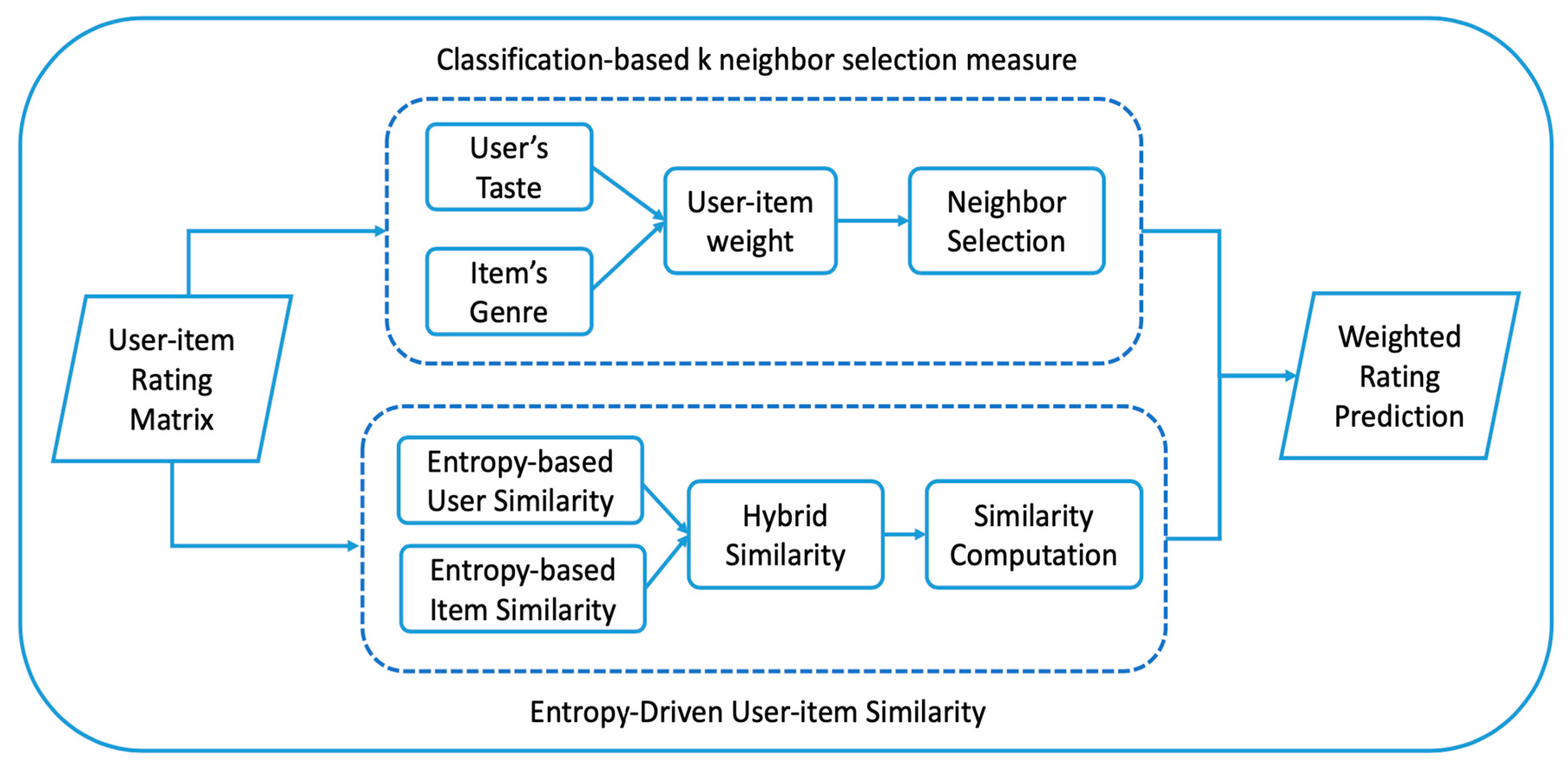
Figure 1. Flow diagram of the proposed model.
Electronics 12 00402 g001
Figure 2. Prediction accuracy obtained using different methods for the ML-100k dataset. MAE—mean absolute error, RMSE—root mean square error.
Electronics 12 00402 g002
Figure 3. Prediction accuracy obtained using different methods for the ML-latest-small dataset. MAE—mean absolute error, RMSE—root mean square error.
Electronics 12 00402 g003
Figure 4. Prediction accuracy obtained using different methods for the ML-1m dataset. MAE—mean absolute error, RMSE—root mean square error.
Electronics 12 00402 g004
Figure 5. Sparsity of the weight matrices versus the number of users.
Electronics 12 00402 g005
Table 1. Details of the datasets.
DatasetNo.RatingsNo.Users N o .   I t e m s R a t i n g   S c a l e Density
ML-100k100,00094316821 to 56.30%
ML-latest-small100,83661097420.5 to 51.70%
ML-1m1000,209604039001 to 54.25%
Disclaimer/Publisher’s Note: The statements, opinions and data contained in all publications are solely those of the individual author(s) and contributor(s) and not of MDPI and/or the editor(s). MDPI and/or the editor(s) disclaim responsibility for any injury to people or property resulting from any ideas, methods, instructions or products referred to in the content.