Design and Analysis of an Effective Multi-Barriers Model Based on Non-Stationary Gaussian Random Fields

Abstract

In this paper, we propose an extension to the barrier model, i.e., the Multi-Barriers Model, which could characterize an area of interest with different types of obstacles. In the proposed model, the area of interest is divided into two or more areas, which include a general area of interest with sampling points and the rest of the area with different types of obstacles. Firstly, the correlation between the points in space is characterized by the obstruction degree of the obstacle. Secondly, multiple Gaussian random fields are constructed. Then, continuous Gaussian fields are expressed by using stochastic partial differential equations (SPDEs). Finally, the integrated nested Laplace approximation (INLA) method is employed to calculate the posterior mean of parameters and the posterior parameters to establish a spatial regression model. In this paper, the Multi-Barriers Model is also verified by using the geostatistical model and log-Gaussian Cox model. Furthermore, the stationary Gaussian model, the barrier model and the Multi-Barriers Model are investigated in the geostatistical data, respectively. Real data sets of burglaries in a certain area are used to compare the performance of the stationary Gaussian model, barrier model and Multi-Barriers Model. The comparison results suggest that the three models achieve similar performance in the posterior mean and posterior distribution of the parameters, as well as the deviance information criteria (DIC) value. However, the Multi-Barriers Model can better interpret the spatial model established based on the spatial data of the research areas with multiple types of obstacles, and it is closer to reality.

1. Introduction

The spatial data often includes location and associated attribute information of interest. Spatial data analysis [1,2] is the process of extracting the spatial data or generating a set of new information about the geographical features to inspect, evaluate, analyze, or model the data in the given areas. The establishment of a spatial analysis model for the spatial data facilitates the estimation and prediction of the spatial data, as well as interpretation and enhanced understanding of the data. Spatial data analysis has been extensively applied to different research fields, such as ecology [3], geology [4], epidemiology [5], industrial IoT [6], engineering [7] and public health [8,9,10].

Spatial Gaussian fields are widely used as spatial components of various spatial or spatiotemporal models. These spatial components are often utilized to explain the spatial structure effects that cannot be directly measured. If there are no suitable covariates in the spatial analysis, only the intercept and spatial Gaussian fields are included in the spatial regression model [11].

Spatial Gaussian random fields, also referred to as Gaussian fields or Gaussian random fields, are stable, i.e., they are invariant to the changes of spatial location or direction. Stationary Gaussian fields are used in spatial modelling because the data are generally assumed to be either stationary, or the non-stationary factors in the data are explainable by other spatial covariates. However, if obstacles, such as lakes, swamps and islands, exist, the stationary model may become inconsistent with the reality; hence, non-stationary models are required.

In the spatial statistics, the closer the distance, the stronger the correlation. It is relevant in cases where there is no obstacle in the area of interest. However, if there are obstacles, the correlation might not be necessarily strong, even if their distances are very short. To address this issue, Bakka [11] proposed the barrier model in 2018. In this model, the spatial dependence between two points is not directly measured by their shortest distance. If the path of the shortest distance between the two points passes through an obstacle, the obstacle also needs to be incorporated in the model to select an appropriate correlation distance for the obstacle area. This model is, however, able to use for one type of obstacle, and only a single correlation distance can be defined for the obstacle area. For complex areas of interest with multiple types of obstacles, different locations with the same distance might have different correlations. Therefore, it is necessary to define different correlation distances for different obstacle areas.

In this paper, we propose the Multi-Barriers Model, which could model the areas of interest with multiple types of obstacle barriers and specify their corresponding correlation distances.

The remainder of the paper is organized as follows. Section 2 describes the related work. Section 3 introduces the basic spatial regression model. Section 4 describes the improved model, i.e., the Multi-Barriers Model. Section 5 and Section 6, respectively, provide the experimental analysis and the performance analysis. Finally, Section 7 ends this paper with a few concluding remarks.

2. The Related Work

In the spatial analysis, the location of the spatial data is known. The spatial data represent a realization of the random process, which is defined as follows:

$$Y\left(s\right)\equiv \left\{y\left(s\right),s\in D\right\},$$

(1)

where $D$ represents a subset of the two-dimensional space and $y\left(s\right)$ represents the observed data at the location $s$.

2.1. Geostatistical Data Regression Model

Geostatistical data, which are the realization of the continuous spatial process $y\left(s\right),$ are the observation results of the location, and $s$ is in the continuous spatial space. The location of s usually refers to a two-dimensional vector expressed by a longitude and a latitude. The actual observation data collection is expressed as $y=\left(y\left(s_1\right),y\left(s_2\right),\dots ,y\left(s_n\right)\right)$, where the collection $\left(s_1,s_2,\dots ,s_n\right)$ represent the locations of the data points.

To analyze the geostatistical data, a spatial regression model is required:

$$\begin{array}{c}y\left(s_i\right)~N\left(\mu \left(s_i\right),{\sigma }^2\right)\hfill \\ \mu \left(s_i\right)~{\beta }_0+{\beta }_1{x}_1+z\left(s_i\right)\hfill \\ z\left(s\right)~N\left(0,\Sigma \right),\end{array}$$

(2)

In Equation (2), it is assumed that the observed value $y\left(s_i\right)$ at each location follows a normal distribution with a mean of $\mu \left(s_i\right)$ and a standard deviation of $\sigma$, and a spatial regression model is established for $\mu \left(s_i\right)$. In Equation (2), ${\beta }_0$ represents the intercept, $x_1$ denotes the covariate related to the mean $\mu \left(s_i\right)$, and ${\beta }_1$ is the weight of the covariate $x_1$. In addition, $z\left(s\right)$ is the continuous spatial Gaussian process (Gaussian random fields), which is used to capture the spatial correlation among the geostatistical data. It is assumed that $z\left(s\right)$ also follows a Gaussian distribution with a mean value of 0 and a covariance matrix of $\Sigma$. In building the spatial regression model, $\Sigma$ is added with the spatial dependence structure to capture the spatial correlation. The Matern correlation function is often adopted to define the spatial dependence structure, so $\Sigma$ is:

$$\Sigma ={\mathit{cov}}_{Matern}(U\left(s_i\right),U\left(s_j\right))={\sigma }_z^2\times co{r}_{Matern}\left(U\left(s_i\right),U\left(s_j\right)\right),$$

(3)

$$co{r}_{Matern}\left(U\left(s_i\right),U\left(s_j\right)\right)=\frac{2^{1-v}}{\Gamma \left(v\right)}\times {(\kappa \times ||s_i-s_j||)}^v\times K_v\left(\kappa \times \left|\right|s_i-s_j\left|\right|\right),$$

(4)

where ${\sigma }_z^2$ is the variance, $K_v$ is the modified Bessel function of the second kind; with $v>0$, $\kappa$ is a scale parameter that controls the decay rate of correlation between the two points. The higher the value of $\kappa$, the faster the correlation decay (see Figure 1). In the above, $\left|\right|s_i-s_j\left|\right|$ is the Euclidean distance between $s_i$ and $s_j$, and the correlation between $s_i$ and $s_j$ is decreased by increasing the distance between them (see Figure 1).

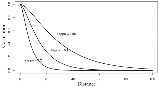
Figure 1. Matern correlation function curves corresponding to different values of $\kappa$.

2.2. Point Pattern

The point pattern is the realization of the point process, where $y\left(s\right)$ indicates whether the event has occurred or not, and it takes the value of 0 or 1. The location of the event is random (e.g., theft incident), and the location, $s,$ where the event took place consists of a longitude and a latitude. To investigate the process of generating these points, it is necessary to build a spatial model for the point pattern, e.g., a log-Gaussian Cox process (LGCP).

The log-Gaussian Cox process is a model that is often used to characterize the environmental changes that cannot be directly measured [12,13]. The point process of the model conformed to a Poisson Model with uneven strength $\lambda \left(s\right)$, i.e., the number of points in the area of interest, $D\in \Omega$, follows a Poisson process with a mean of $\Lambda \left(D\right)$, where

$$\Lambda \left(D\right)={\int }_D\lambda \left(s\right)ds,$$

(5)

and $\lambda \left(s\right)$ denotes the intensity of the point process. This model is also used to characterize the aggregation of points or events caused by the observed and unobserved environmental changes. In this paper, a log-Gaussian Cox model is applied, where

$$\mathit{log}(\lambda \left(s\right))={\beta }_0+Z\left(s\right),$$

(6)

and ${\beta }_0$ represents the global mean of the logarithmic intensity, and $Z\left(s\right)$ represents a Gaussian random field. Therefore, the log-Gaussian Cox model becomes a latent Gaussian model, so the model can be fitted under a hierarchical Bayesian framework. The covariate can also be added to the model to investigate the distribution law of the points in space. Two methods for obtaining $Z\left(s\right)$ are presented in the following.

2.2.1. Traditional Methods

The traditional method of inferring LGCP is based on dividing the area of interest, $\Omega$, into small non-overlapping grids [14,15] and then counting the number of points ($N_{ij}$) in each grid $S_{ij}$. The number of points in each grid follows a Poisson distribution:

$$N_{ij}~Possion\left(\lambda \left(s_{ij}\right)\right),$$

(7)

$$\lambda \left(s_{ij}\right)={\int }_{s_{ij}}\lambda \left(s\right)ds,$$

(8)

where $\lambda \left(s_{ij}\right)$ is the intensity of $s_{ij}$. Since obtaining the intensity of each grid point with the integral method requires many computations, an approximated solution method is used to obtain the integral in Equation (8) as:

$$\lambda \left(s_{ij}\right)\approx \left|\left.s_{ij}\right|\mathit{exp}(z_{ij})\right.,$$

(9)

where $z_{ij}$ is the value of $Z\left(s\right)$ in the grid $s_{ij}$, and $\left|\left.s_{ij}\right|\right.$ denotes the area of the grid $s_{ij}$. In this method, it is assumed that the intensity of points is uniform within each grid but different in each grid. This model can be fitted as a generalized linear mixed model as an approximation of the real model, where the grid is finely divided. This method has been widely used in the related literature. However, since $Z\left(s\right)$ is an ordinary Gaussian random field, the covariance matrix of the multivariate Gaussian vector $,z,$ is dense. Therefore, the computational complexity is significantly increased by increasing the increase in the grid.

2.2.2. Stochastic Partial Differential Equation (SPDE) Method

In addition to the traditional methods, the SPDE method is also used to approximate the Gaussian random field Z(s). It is a relatively new approach to applying the SPDE in the geostatistical models. The SPDE was first proposed by Whittle [16] in 1954 and then further extended by Lindgren et al. [17] in 2011. Thereafter, the method has been extended and applied to many different problems. In this paper, the solution of the SPDE is a Gaussian random field with Matern covariance function:

$${({\kappa }^2-\Delta )}^{\alpha /2}\tau Z\left(s\right)=W\left(s\right),$$

(10)

where $Z\left(s\right)$ is residual to be calculated, $\Delta$ is the Laplacian operator, and $W\left(s\right)$ is white Gaussian noise in the spatial domain, i.e., there is no spatial correlation in W(s). In Equation (10), $\kappa$ is identical to $\kappa$ in the Matern correlation function, and $\alpha$ is a fixed value with $\alpha$ = 2.

Lindgren et al. [17] also proposed that the solution of the SPDE can be approximated using the finite element method. In this method, the Gaussian random field with a dense covariance matrix is substituted with a Gaussian Markov random field with a sparse precision matrix, resulting in a significant improvement in computational efficiency. The finite element method can be expressed as:

$$Z\left(s\right)={\sum }_{i=1}^n{z}_i{\phi }_i\left(s\right),$$

(11)

The area of interest is divided into non-overlapping triangular areas (Figure 2b) using the finite element method. The vertex of each triangle is referred to as a node. By calculating the value of each node, the solution of the SPDE is then expressed using the finite element method, and the approximated distribution of the Gaussian random field is finally obtained. In Equation (11), $z=\left(z_1,z_2,\dots ,z_n\right)$ is a multivariate Gaussian random vector, and ${\left\{\left.{\phi }_i\left(s\right)\right\}\right.}_{i=1}^n$ is a piecewise linear basis function. Using Equations (6) and (11), we then write:

$$\mathit{log}(\lambda \left(s\right))={\beta }_0+{\sum }_{i=1}^n{z}_i{\phi }_i\left(s\right),$$

(12)

Figure 2. Approximation of the real random field using the finite element method: (a) Real random field; (b) Triangular grid; (c) Approximated random field.

Figure 2a: A continuously indexed spatial random field; (b): Division of the research area into non-overlapping adjacent triangles; (c): Approximate spatial random field represented by the finite element on the spatial random field of Figure 2a based on the piecewise linear basis function defined in each triangle grid. The larger the number of grids, the closer the approximate spatial random field to the real spatial random field.

2.3. Integrated Nested Laplace Approximation (INLA)

In this paper, the INLA algorithm is used to calculate the parameters of the geostatistical model and log-Gaussian Cox model to obtain the posterior mean and posterior distribution of the model parameters. The INLA [18] is a method of statistical inference of latent Gaussian models, which provides a rapid and accurate inference method for the marginal posterior distribution of Bayesian parameters and hyperparameters. To avoid the time-consuming Markov chain Monte Carlo simulation, we directly use a series of Laplace approximation methods to calculate the posterior density of the latent Gaussian model. The posterior distribution of hyperparameters is obtained as the following:

$$\tilde{\pi }(x_i|y)=\int \tilde{\pi }(x_i|\theta ,y)\tilde{\pi }(\theta |y)d\theta \approx {\sum }_{k=1}^K\tilde{\pi }(x_i|{\theta }_k,y)\tilde{\pi }({\theta }_k|y){\Delta }_k,$$

(13)

The posterior margin of the hyperparameter $\tilde{\pi }\left(x_i,y\right)$ can be obtained using numerical integration in which the selection of integration point ${\theta }_k$ affects the accuracy and calculation efficiency of INLA results. There are two methods for selecting the integration points, grid integrated divide (GRID) and central command divide (CCD) strategies. The GRID strategy defines a grid that covers most the areas of $\tilde{\pi }(\theta |y)$. This method is more accurate, but it is more time-consuming. The CCD strategy selects a small number of data points to estimate $\tilde{\pi }(\theta |y)$. This method is fast and accurate enough. The results of INLA refer to the marginal distribution of a series of parameters and hyperparameters through which the mean, variance and quantile of the distributed parameters and hyperparameters are calculated; hence, the statistical information of interest is obtained.

3. The Basic Spatial Regression Model

Stationary Gaussian random fields are used in the spatial analysis; in practice, however, it is unreasonable to utilize stationary Gaussian random fields as there are often obstacles to the spatial analysis of certain types of spatial data. For example, an island is considered as an obstacle for the fishes. Because fishes cannot leave the water, it is thus impossible for them, on one side of the island, to have correlations with the fish on the other side by crossing the island in a straight line. Therefore, the correlation between the fishes around the island cannot be defined by the length of the straight line between them. Similarly, for plants or animals that live on the land, the lakes and rivers are obstacles because these species cannot survive in the water. Therefore, in such cases, the model should be built using a non-stationary Gaussian random field.

In 2018, Bakka et al. proposed the barrier model that divided the area of interest into two parts: one is the ordinary area of interest (i.e., the sampling area), and the other is the obstacle area. In building the model, the stochastic partial differential functions were then constructed for the general area of interest and the obstacle area:

$$\begin{gathered} z\left(s\right)-\mathsf{\nabla }\cdot \frac{r^2}{8}\mathsf{\nabla }z\left(s\right)=r\sqrt{\frac{\pi }{2}}{\sigma }_{z}W\left(s\right),fors\in \Omega \\ z\left(s_b\right)-\mathsf{\nabla }\cdot \frac{r_b^2}{8}\mathsf{\nabla }z\left(s_b\right)=r\sqrt{\frac{\pi }{2}}{\sigma }_{z}W\left(s_b\right),for{s}_b\in {\Omega }_b, \end{gathered}$$

(14)

$$r_b=r\rho ,$$

(15)

Equation (14) consists of two SPDEs for the general area of interest and the obstacle area, where $\Omega$ represents the general research area; ${\Omega }_b$ denotes the obstacles, such as lakes, islands and swamps; and $z\left(s\right)$ and $z\left(s_b\right)$ stand for the Gaussian fields of the general area of interest and the obstacle area, respectively. In Equation (14), $\mathsf{\nabla }=\left(\left.\frac{\partial }{\partial x},\frac{\partial }{\partial y}\right)\right.$ is the gradient; $r$ and $r_b$ refer to the correlation distance of the general area of research $\Omega$ and the obstacle area ${\Omega }_b$, respectively; ${\sigma }_z$ is the standard deviation of the Gaussian field; and $W\left(s\right)$ is white noise. The relationship between the correlation distance $r_b$ in the obstacle area and the correlation distance $r_b$ in the general area of interest is shown in Equation (15). It can be seen that the correlation distance $r$ in the obstacle area is the product of the correlation distance $r$ in the general research area and the threshold $\rho$.

The respective random fields are then obtained through solving the two SPDEs in Equation (14). There are, however, certain limitations attributed to this model. For instance, there may be more than one obstacle in the actual area of interest, and the effect of various obstacles on the correlation between the points may be different. Nevertheless, different types of obstacles are simply regarded as the same type of obstacles. To address this issue, in this paper we extended this model to create the Multi-Barriers Model. The extended model specifies different thresholds for different types of obstacles to represent their corresponding effect on the correlations and further enhance the validity and application range of the model.

4. Multi-Barriers Gaussian Random Fields

4.1. Mathematical Model

In this paper, we extend the barrier model to be adaptable to multiple types of obstacles. Different types of obstacles exert different effects on the correlation; hence, characterizing their impacts will significantly improve the model accuracy and applicability.

The Multi-Barriers Model divides the area of interest into multiple categories, including the general area of interest, and various obstacle areas and establishes multiple SPDEs as the following:

$$\begin{array}{l}z\left(s\right)-\mathsf{\nabla }\cdot \frac{r^2}{8}\mathsf{\nabla }z\left(s\right)=r\sqrt{\frac{\pi }{2}}{\sigma }_{z}W\left(s\right),fors\in {\Omega }_0\\ z\left(s_1\right)-\mathsf{\nabla }\cdot \frac{r_1^2}{8}\mathsf{\nabla }z\left(s_1\right)=r_1\sqrt{\frac{\pi }{2}}{\sigma }_{z}W\left(s_1\right),for{s}_1\in {\Omega }_1\\ z\left(s_2\right)-\mathsf{\nabla }\cdot \frac{r_2^2}{8}\mathsf{\nabla }z\left(s_2\right)=r_2\sqrt{\frac{\pi }{2}}{\sigma }_{z}W\left(s_2\right),for{s}_2\in {\Omega }_1\\ \dots \\ z\left(s_n\right)-\mathsf{\nabla }\cdot \frac{r_n^2}{8}\mathsf{\nabla }z\left(s_n\right)=r_n\sqrt{\frac{\pi }{2}}{\sigma }_{z}W\left(s_n\right),for{s}_n\in {\Omega }_n,\end{array}$$

(16)

$$r_1=r{\rho }_1,r_2=r{\rho }_2,\dots ,r_n=r{\rho }_n,$$

(17)

where there are $n+1$ SPDEs, which represent the general area of interest ${\Omega }_0$, and $n$ types of obstacle are the relations of the correlation distance $r$ to the general area of interest $\Omega$ and $n$ types of obstacle area ${\Omega }_{1-n}$, respectively. In this formulation, ${\sigma }_z$ also indicates the standard deviation of the Gaussian field, and $W\left(s\right)$ is white noise. The correlation distance $r_1,r_2,\dots ,r_n$ in the obstacle areas and the correlation distance in the general area of interest are presented in Equation (17), where ${\rho }_1,{\rho }_2,\dots ,{\rho }_n$ represent the corresponding thresholds.

To approximate the solution of the SPDEs using the finite element method, the area of interest is divided into non-overlapping adjacent triangle areas, where the triangles in the areas ${\Omega }_a$ and ${\Omega }_b$ are independent. As is shown in Figure 3b, the areas enclosed by the red and blue rectangles are the obstacle areas, and the small triangles in the red and blue rectangles are independent of those in the general area of interest. The respective random fields, $z\left(s\right)$, are obtained by solving $n+1$ SPDEs. The number of parameters in this model is the same as the stationary Gaussian model. In this model, $r_1,r_2,\dots ,r_n$ in the obstacle area are obtained by multiplying ${\rho }_1,{\rho }_2,\dots ,{\rho }_n$ and $r$ in the general area of interest, and ${\rho }_1,{\rho }_2,\dots ,{\rho }_n$ specify the corresponding numerical values for the obstruction degree to the correlation of the model, which are based on different types of the obstacle areas.

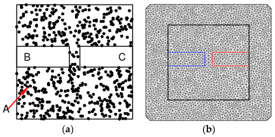
Figure 3. Simulation scenario: (a) Research area and data; (b) Triangular grid. Note: Area A in (a) represents the general area of interest, and areas B and C are two different types of obstacles.

4.2. Model Comparison

Here, we illustrate the effect of the obstacle areas on the stationary Gaussian model, the barrier model and the Multi-Barriers Model on the correlation between the points in the general area of interest. Here, the sample data are generated using simulation, and a comparative test is performed for the three models based on the sample data. Furthermore, a point is selected from the general area of interest to investigate the changes in the correlation at this point along with the change of location in each model.

According to the area of interest shown in Figure 3a, as well as the location information and numerical information of the geostatistical data generated by simulation, the spatial regression models are established using the stationary Gaussian model, the barrier model (that is, the non-stationary Gaussian model) and the Multi-Barriers Model. The three models are calculated using the INLA method to obtain the posterior distribution of the parameters and hyperparameters of each model. Based on these, the statistics of each parameter and hyperparameter are then obtained. Moreover, the changes in the correlation between the points in each model are simulated by the statistics of the posterior distribution of parameters and hyperparameters (such as mean and variance). A point is then selected from the area of interest to simulate the changes in the correlation between this point and other areas in the three models where the spatial location is changed. We then compare the differences between these three models. The distance between two types of obstacle areas in the area of interest is continuously reduced to illustrate the changes in the correlation between the selected point and other areas (Figure 4).

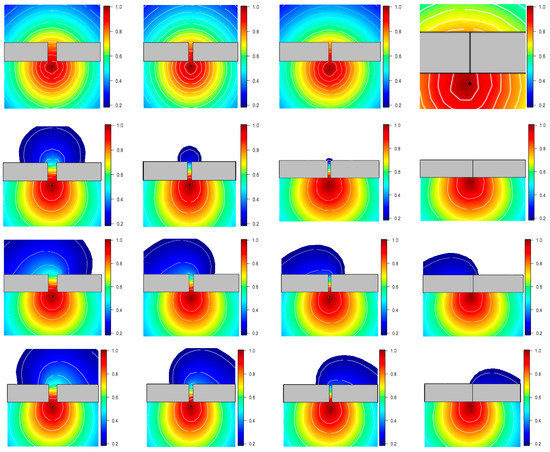
Figure 4. Changes in the correlation between the points in the three models in the areas. Note: The four graphs in the first row represent the changes in the correlation between the points in the stationary Gaussian model and those in the second row display the changes in the correlation between the points in the barrier model. The graphs in the third and fourth rows manifest the changes in the correlation between the points in the Multi-Barriers Model under different thresholds. The distances between the obstacles in the first column and the fourth column are 1, 0.5, 0.3, and 0, respectively.

In Figure 4, the graphs in the first row represent the changes in the correlation between points changes in the correlation between the points generated by the Multi-Barriers Model, where the thresholds of the obstacle areas are different. The threshold of the obstacle area on the left of the third row was 0.5 and that on the right was 0.0001. It is seen that the obstacle area on the left has a smaller obstructing effect on the correlation between the points in the general area of interest. In the fourth row, the threshold of the left obstacle area is 0.0001, while that of the right obstacle area is 0.5. These suggest that the left obstacle area has a greater obstructing effect on the correlation between the points in the general research area. The distances between the two columns of obstacles in the graphs are 1, 0.5, 0.3, and 0, respectively. By decreasing the distance between the obstacle areas, the correlation between the points below the area of interest and the area above the area of interest becomes smaller. If the distance between the obstacle areas becomes 0, the correlation between the points below the area of interest and the area above it has its smallest value.

5. Experimental Analysis

In this section, the spatial regression model is established for the comparative analysis of parameters by applying the stationary Gaussian model, barrier model and Multi-Barriers Model to the geostatistical data and point data. Using these models, we then evaluate the performance of the models. Note that the geostatistical data and the research area are all obtained through simulation, and the point data are taken from the real data sets of burglary incidents in a certain area.

The simulations of the proposed method are implemented by Python. All the experiments are carried out on a computer with an Intel (R) Core (TM) i5 processor running at 2.80 GHz.

5.1. Simulation Experiment of Geostatistical Data

5.1.1. Data Simulation

To investigate the similarities and differences amongst the stationary Gaussian model, the barrier model and the Multi-Barriers Model, a spatial regression model is established for the three models in the simulated research area. In addition, two different types of obstacle areas are considered in the area of interest to compare these three models. We then set:

$$y=Intercept+z,z~N\left(0,\Sigma \right),$$

(18)

where $y$ is the numerical value of the data point.

In this experiment, the $y$ value of each sampling point is obtained by the simulation generation method, and then it is fitted using the stationary Gaussian model, the barrier model and the Multi-Barriers Model. Intercept stands for the intercepting, and $z$ is a Gaussian random field with Matern covariance. It is seen that Equation (18) is a latent Gaussian model, which can be calculated by the INLA method.

The area of interest in this experiment is a 10 × 10 square area, and two rectangles of the same size are selected as different types of obstacle areas. The sampling points are also obtained using a random generator and the corresponding y value is given for each sampling point according to a certain set of rules. The 558 data points are obtained, see Figure 5a, where a blue point indicates a positive data point, and the larger the point, the higher the numerical value. Moreover, the red point indicates a negative data point, and, similarly, a larger red point means a lower data value. The area of A is the general interest area; the areas of B and C are two different types of obstacle areas. We further assume that there is no sampling point in the obstacle areas.

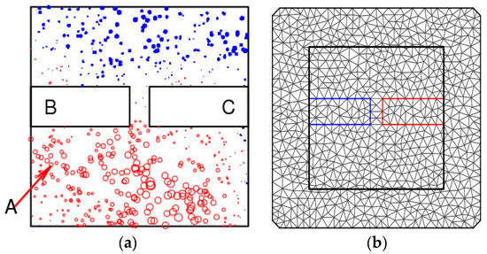
Figure 5. Simulated data: (a) Simulated research area and data points; (b) Triangular grid. Note: area A in (a) is the general area of interest, and areas B and C are two different types of obstacle areas.

To obtain the covariance matrix of the Gaussian random field z, the solution of SPDEs are obtained using the finite element method. Therefore, the research area in Figure 5a is divided into small adjacent and non-overlapping triangles as in Figure 5b. It is shown in Figure 5b that the triangles in the general area of interest and the obstacle area are adjacent to, but independent of, each other. Adopting the barrier model or the Multi-Barriers Model, the SPDEs are separately established for the general area of interest and the obstacle area to obtain different results.

5.1.2. Parameter Analysis

Here, we establish the stationary Gaussian random model, barrier model, and Multi-Barriers Model for the sample data obtained through simulation. The models are then calculated using the integrated Laplace approximation method to obtain the posterior distribution of parameters of each model (see Figure 6). The first to the third columns in Figure 6 exhibit the posterior distribution of parameters ${\sigma }_z$, $\kappa$ and Range, respectively, and the fourth column displays the Matern correlation function curves calculated from the posterior mean of the parameter $\kappa$. Each row in Figure 6 represents one model or the same model under different thresholds. The first row shows the posterior distribution of parameters and the correlation function curves of the stationary Gaussian model. The second row further illustrates the posterior distribution of parameters and the correlation function curves of the barrier model. Moreover, the third and fourth rows manifested the posterior distribution of parameters and the correlation function curves of the Multi-Barriers Model. Nevertheless, the thresholds specified for the two types of obstacle areas are different between the third and fourth rows (Table 1).

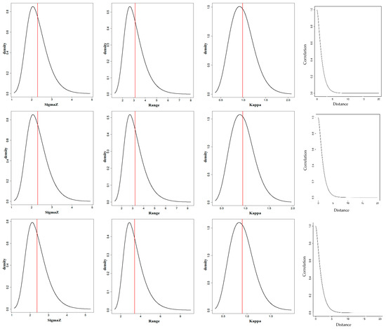
Figure 6. Posterior distribution of the parameters and Matern correlation function of the models. Note: The first and second rows represent the posterior distribution of parameters and the Matern correlation function curves of the stationary Gaussian model and the barrier model, and the third and fourth rows illustrate the posterior distribution of parameters and the Matern correlation function curves of the Multi-Barriers Model under different threshold values. The vertical line in the graphs indicates the posterior mean of the parameter.

Table 1. Posterior mean, threshold and deviance information criteria (DIC) value for the parameters of each model.

	Stationary Gaussian Model	Nonstationary Gaussian Model (Barrier Model)	Nonstationary Gaussian Model 1 (Multi-Barriers Model)	Nonstationary Gaussian Model 2 (Multi-Barriers Model)
Threshold value 1 (${\rho }_1$)	-	0.001	0.15	0.001
Threshold value 2 (${\rho }_2$)	-	0.001	0.001	0.15
Intercept	0.32	0.34	0.32	0.24
${\sigma }_z$	2.76	2.54	2.55	2.54
$\kappa$	0.29	0.32	0.32	0.32
Range	10.13	9.26	9.28	9.27
Range1	10.13	0.00926	1.392	0.00927
Range2	10.13	0.00926	0.00928	1.39
DIC	1054.47	1053.09	1053.1	1053.12

In Table 1, Intercept is the intercept value, ${\sigma }_z$ is the standard deviation of the Gaussian random fields and $\kappa$ is the scale parameter in the Matern correlation function, which controls the decay rate of the correlation between the points with the increasing distance. Both ${\rho }_1$ and ${\rho }_2$ are thresholds representing the correlation distance of the obstacle area is a multiple of the correlation distance of the general research area. Range is the correlation distance of the general area of interest A in Figure 4, and Range1 and Range2, which are the correlation distances between the obstacle areas B and C in Figure 6, are calculated by multiplying the correlation distance of the general research area A (Range) and the corresponding threshold values ${\rho }_1$ and ${\rho }_2$. The value of the deviance information criteria (DIC) is also utilized to measure the model performance and is defined as:

$$DIC=goodnesoffit+complexity=D\left(\left.\overline{\theta }\right)+2p_D\right.,$$

(19)

where $D\left(\overline{\theta }\right)$ is the biased estimation of the posterior mean of the parameters. The larger the value of $D\left(\overline{\theta }\right)$, the greater the model deviation. In Equation (19), $p_D$ is the number of effective parameters, indicating the complexity of the model, where a more complex model possesses more effective parameters.

The smaller the numerical value of DIC, the better the model. Figure 6 and Table 1 also suggest that the standard deviation ${\sigma }_z$ of the stationary Gaussian model is slightly higher than that of the barrier model and the Multi-Barriers Model, whereas $\kappa$ is slightly lower than that of the other two models. Therefore, the stationary Gaussian model has a slightly lower decay rate of correlation than that of the other two models. However, the posterior distribution and posterior mean of each parameter between the barrier model and the Multi-Barriers Model are similar. The difference in the DIC value is very low among the three models. This suggests that the overall performance of the three models is close to each other.

The posterior means of the spatial random fields of the stationary Gaussian model, the barrier model and the Multi-Barriers Model are also obtained using the integrated Laplace approximation and shown in Figure 7. Figure 7a illustrates the posterior mean of the spatial random field, resulting from the stationary Gaussian model. Figure 7b shows the posterior mean of the spatial random field, resulting from the calculation of the barrier model using the integrated Laplace approximation. Since the barrier model treats all the obstacles similarly, the correlation distances of different types of obstacle areas remain the same. The threshold value adopted in this paper is 0.001, i.e., namely, ${\rho }_1={\rho }_2=0.001$ Table 1), so the correlation distance in the obstacle area in Figure 7b is 0.001 times the general area of interest. It is also seen in Figure 7b that the correlation between the points in the general research area is rapidly reduced to 0 by passing through the obstacle area. For the spatial random fields of the spatial locations without sampling points, their numerical value in the obstacle area is 0. These points are obtained using a spatial model fitting of data information from the sampling points. There is no data information in the obstacle area and the correlation of data between the obstacle area and the general research area is very low.

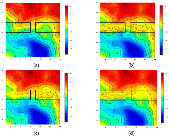
Figure 7. Spatial random fields of different models. (a) Spatial random field of the stationary Gaussian model; (b) Spatial random field of the barrier model; (c) Model spatial random field of the Multi-Barriers Model; (d) Spatial random field of the Multi-Barriers Model.

Figure 7c,d demonstrate the posterior means of the spatial random fields of the Multi-Barriers Model. The two models only differ in the threshold value. By the modification of the barrier model, the Multi-Barriers Model specifies the same or different thresholds for different types of obstacles as required. The thresholds of the left and right obstacles in Figure 7c are 0.15 and 0.001, respectively (i.e., ${\rho }_1$ = 0.15, ${\rho }_2$ = 0.001). Furthermore, the thresholds of the left and right obstacles in Figure 7d are 0.001 and 0.15, respectively (i.e., ${\rho }_1$ = 0.001, ${\rho }_2$ = 0.15). It is also seen from Figure 7c that the decay rate of correlation in the obstacle area on the left is slightly lower than that in Figure 7b,d, but it is higher than that in Figure 7a. Moreover, the decay rate of correlation in the obstacle area on the right in Figure 7c is roughly identical to that in Figure 7b. The correlation between the points in the general area of interest is quickly decayed to zero by passing through the obstacle area on the right. The situation in Figure 7d is the opposite of Figure 7c. In Figure 7d, the correlation in the right obstacle area slowly decayed compared to that in the left obstacle area.

Therefore, different types of obstacle areas make different impacts on the correlation between points in the area of interest. For instance, rocky areas and wetlands may affect the correlation between trees as the tree roots are unable to pass through the rocks but can pass through wetlands. Therefore, a larger threshold should be associated with the wetlands. Therefore, it is necessary to specify different thresholds for different obstacle areas to make the spatial model more efficient.

5.2. Point Pattern Data

5.2.1. The Data and Area of Interest Introduction

Burglary incidents are violent crimes in which the properties of others are infringed. To build a harmonious social environment and improve the level of public safety, it is essential to plot the main areas with a high frequency of burglary to understand the crime patterns. In this section, 175 cases of burglary incidents occurred in a street in 2016 are projected into a model using the log-Gaussian Cox model, see Figure 8a. Since the burglary incidents only occur in residential areas, such as communities and villages, it is unlikely to have such incidents in areas, such as lakes and meadows. In addition, these areas may hinder the correlation between the locations of burglary, and further, obstruct the spatial correlation between burglary cases. Different types of obstacles also have different obstructing effects on the occurrence of burglary incidents. Therefore, such obstacles should be incorporated into the model.

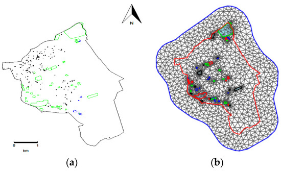
Figure 8. Area of interest and its corresponding mesh: (a) Area of interest and two types of obstacle areas; (b) Triangular grid. Note: (a) The area enclosed by the green line indicates the meadow, the area enclosed by the blue line illustrates the water system area and the black dots indicate the location of burglaries.

In this section, the log-Gaussian Cox model combined with the Multi-Barriers Model is applied to establish a model for the burglary cases. It is then compared with the ordinary log-Gaussian Cox model and log-Gaussian Cox model combined with the barrier model.

There are two types of obstacles in the area of interest, see Figure 8: The area surrounded by the green line is the meadow, and the area surrounded by the blue line is the water system. The black dots represent the locations where burglary incidents were reported.

5.2.2. Parameters Analysis

In this section, a log-Gaussian Cox model with stationary Gaussian random fields and a log-Gaussian Cox model with non-stationary Gaussian random fields (i.e., barrier model and Multi-Barriers model) are established for the burglary data in a certain area. The models are calculated by the integrated Laplace approximation method to obtain the posterior distribution of the parameters of each model (Figure 9). The first, second and third columns in Figure 9 illustrate the posterior distribution of parameters ${\sigma }_z$, $\kappa$ and Range, respectively, and the Matern correlation function curves are plotted based on the calculation of the posterior mean of the parameter $\kappa ,$ which is shown in the fourth column. Each row in Figure 9 is associated with one model. The first, second and third rows illustrate the posterior distribution of parameters and the correlation function curves of the stationary Gaussian model, the barrier model and the Multi-Barriers model, respectively, and the posterior means of the parameters are shown in Table 2.

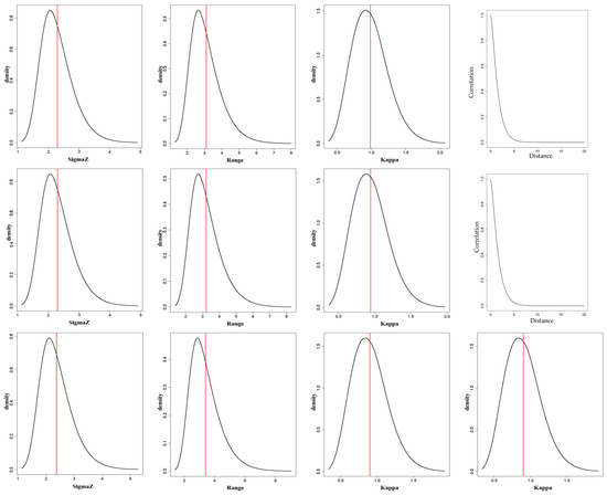
Figure 9. Posterior distribution of parameters and Matern correlation function for the three models. Note: The first, second and third rows show the posterior distribution of the parameters and the Matern correlation function of the stationary Gaussian model, the barrier model and the Multi-Barriers Model, respectively.

Table 2. Posterior mean, threshold and DIC values of parameters of the three considered models.

	Stationary Gaussian Model	Nonstationary Gaussian Model (Barrier Model)	Nonstationary Gaussian Model (Multi-Barriers Model)
$\mathrm{Threshold}\mathrm{value}1({\rho }_1$)	-	0.02	0.02
$\mathrm{Threshold}\mathrm{value}2({\rho }_2$)	-	0.02	0.1
Intercept	−0.18	−2.00	−1.46
${\sigma }_z$	2.29	2.30	2.38
$\kappa$	0.98	0.94	0.90
Range (km)	3.10	3.22	3.40
Range1 (km)	3.10	0.064	0.068
Range2 (km)	3.10	0.064	0.34
DIC	−783.18	−782.91	−773.73

The parameters in Table 2 convey the same meaning as those in Table 1. Comparing the posterior distribution of the parameters for the three considered models in Figure 9 and the posterior means of parameters in Table 2, it is seen that the parameters and DIC values of these models are close. However, the Intercept of the stationary Gaussian model is slightly higher than that of the other two models. Burglary cases only occur in places where people live; hence, meadows and water areas have obstructing effects on the correlation between the locations of burglary. This is because few criminals may travel across the meadows or water system to commit their crimes. Hence, the actual situations should be taken into account when constructing the model. Therefore, the log-Gaussian Cox model with non-stationary Gaussian random fields is more appropriate.

6. Performance Analysis

Nevertheless, different obstacle areas, such as meadows and water areas, have various degrees of obstruction effect on the correlation between the locations of burglary. For instance, criminals are more likely to walk across a meadow to commit a crime than to swim through a lake. In this case, the log-Gaussian Cox model with multiple types of obstacles and non-stationary Gaussian random fields might be more suitable. As it is shown in Table 2, the thresholds of the two types of obstacle areas are 0.02 and 0.1, respectively (i.e., ${\rho }_1$ = 0.02, ${\rho }_2$ = 0.1), and the water areas may have a higher obstruction effect on the correlation between the locations of burglaries.

The spatial random fields of the three considered models are displayed in Figure 10. The first graph (Figure 10a) illustrates the posterior mean of the spatial random field of the log-Gaussian Cox model with stationary Gaussian random fields (i.e., the obstruction of the obstacle areas to the correlation between the locations of burglary is not considered). The second graph (Figure 10b) shows the posterior mean of the spatial random field of the log-Gaussian Cox model with non-stationary Gaussian random fields (barrier model). The same threshold (${\rho }_1={\rho }_2$ = 0.02) is considered for the two types of obstacle areas in this model. In other words, it is assumed that the meadows and water areas have a similar obstruction effect on the correlation between the locations of burglaries. Furthermore, the correlation distances in the two types of obstacle areas (Range1 and Range2), which are both equal to 0.064 km, are the respective products of the threshold values of the two types of obstacle areas and the correlation distance Range of the general area of interest. It is also found that the correlation between the points in the general research area is quickly decayed to 0 by passing through the obstacle area (Figure 10b), so the spatial random field in the obstacle area is 0. The third graph (Figure 10c) further illustrates the posterior mean of the spatial random field of the log-Gaussian Cox model with non-stationary Gaussian random fields (Multi-Barriers Model). In this model, varying threshold values (i.e., ${\rho }_1$ = 0.02, ${\rho }_2$ = 0.1) are considered for the two types of obstacle areas. The water areas had a greater obstructing effect on the correlation between the locations of burglaries, and the correlation distances of the water areas and the lawns are 0.068 km and 0.34 km, respectively. Figure 10c suggests that the decay rate of the correlation between the points in the general area of interest is prominently increased when passing through the obstacle area of the meadows, in contrast with passing through the general area of interest.

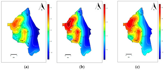
Figure 10. Spatial random fields of different models: (a) Spatial random field of stationary Gaussian model; (b) Spatial random field of barrier model; (c) Spatial random field of Multi-Barriers Model.

7. Conclusions and Future Work

In this paper, the barrier model is extended to create the Multi-Barriers Model. In the extended model, different threshold values are designated for different types of obstacle areas to characterize their corresponding degree of obstruction on the correlation between the points. The proposed model applies to more practical cases scenarios and the corresponding established model is closer to reality.

The Multi-Barriers Model is the same as the barrier model in the range of applications.

However, in the case of multiple types of obstacle, the Multi-Barriers Model with the various thresholds, which are based on the accumulated experiential knowledge, expert advice, or related historical data, could acquire more realistic results. In this paper, the similarities, differences and performance of the stationary model, the barrier model and the Multi-Barriers Model are investigated and are applied to the geostatistical and point pattern data in combination with the experimental data. In the stationary Gaussian model, different types of obstacle areas have no obstructing effect on the correlation between points in the general area of interest. The threshold value is specified for the obstacle areas to obtain the obstructing effect on the correlation between the points in the area of interest in the barrier model. In this model, the obstructing effect of different types of obstacles on the correlation in the general area of interest remained the same. The Multi-Barriers Model enables establishing models for multiple types of obstacles with various degrees of obstruction effects on the correlation in the general area of interest. Moreover, there is no significant difference in the performance between the Multi-Barriers Model and the stationary Gaussian model and the barrier model, but the Multi-Barriers Model is significantly closer to the real situations. Therefore, the model should be established according to the actual situation of the area of interest. If there are no obstacles in the area of interest or the obstacles do not affect the correlation, the stationary Gaussian random field model is considered as a suitable model. The barriers model is a reasonable choice for the cases when there is only one type of obstacle in the area of interest or different types of obstacles with a similar obstructing effect on the correlation. Furthermore, the proposed Multi-Barriers Model is applicable for many different types of obstacles in the research area [19], and such obstacles exert diverse obstructing effects on the correlation. Such scenarios are not covered by the existing model.

References

- Soso, B.; Romero, D.; Fernandez, G. Spatial analysis to identify invasion colonization strategies and management priorities in riparian ecosystems. For. Ecol. Manag. 2018, 411, 195–202. [Google Scholar] [CrossRef]
- Liming, G.; Lele, Z. Spatiotemporal Dynamics of the Vegetation Coverage in Qinghai Lake Basin. J. Geo.-Inf. Sci. 2019, 21, 1318–1329. [Google Scholar]
- Kimpouni, V.; De, N.J.; Massamba-Makanda, C.M. Spatial Analysis of the Woody Flora of the Djoumouna Peri-urban Forest, Brazzaville (Congo). Ecol. Evol. Biol. 2019, 4, 1–3. [Google Scholar] [CrossRef]
- Kuanjia, L.; Yansheng, G.; Manzhou, L.; Lin, L.; Junjie, D.; Zijian, L.; Wen, T. Spatial analysis, source identification and risk assessment of heavy metals in a coal mining area in Henan, Central China. Biodeterior. Soc. 2018, 128, 148–154. [Google Scholar]
- Beiping, W.; Dian, Y.; Jinfeng, W.; Chengdong, X.; Junming, L.; Zhoupeng, R. Space-time Variability and Determinants of Hand, Foot and Mouth in Shandong Province: A Bayesian Spatio-temporal Modeling Approach. J. Geo-Inf. Sci. 2016, 18, 1645–1652. [Google Scholar]
- Fu, A.; Zhang, X.; Xiong, N.; Gao, Y.; Wang, H.; Zhang, J. VFL: A verifiable federated learning with privacy-preserving for big data in industrial IoT. IEEE Trans. Ind. Inform. 2022, 18, 3316–3326. [Google Scholar] [CrossRef]
- Hariri-Ardebili, M.A.; Mahdavi, G.; Abdollahi, A.; Amini, A. An RF-PCE Hybrid Surrogate Model for Sensitivity Analysis of Dams. Water 2021, 13, 302. [Google Scholar] [CrossRef]
- Liqian, S.; Cong-cong, X.; Rui, L.; Yi, H.; Sui-heng, L.; Cheng-long, X.; Zhijie, Z. Spatial distribution characteristics of global highly pathogenic avian influenza H5N1 based on the spatial point pattern analysis. Chin. J. Dis. Control. Prev. 2016, 20, 555–558. [Google Scholar]
- Xiaohui, L.; Yongwei, L.; Fei, C.; Wenping, F. Selection Method for Urban Emergency Medical Institutions Considering Spatiotemporal Accessibility. J. Geo-Inf. Sci. 2019, 21, 1411–1419. [Google Scholar]
- Gao, Y.; Xiang, X.; Xiong, N.; Huang, B.; Lee, H.J.; Alrifai, R.; Jiang, X.; Fang, Z. Human action monitoring for healthcare based on deep learning. IEEE Access 2018, 6, 52277–52285. [Google Scholar] [CrossRef]
- Bakka, H.; Vanhatalo, J.; Illian, J.B.; Simpson, D.; Rue, H. Non-stationary Gaussian models with physical barriers. Spat. Stat. 2019, 29, 268–288. [Google Scholar] [CrossRef]
- Møller, J.; Syversveen, A.R.; Waagepetersen, R.P. Log gaussian cox processes. Scand. Stat. Theory Appl. 1998, 25, 451–482. [Google Scholar] [CrossRef]
- Illian, J.B.; Sørbye, S.H.; Rue, H. A toolbox for fitting complex spatial point process models using integrated nested Laplace approximation (INLA). Ann. Appl. Stat. 2012, 6, 1499–1530. [Google Scholar] [CrossRef]
- Srbye, S.H.; Illian, J.B.; Simpson, D.P. Careful prior specification avoids incautious inference for log-Gaussian Cox point processes. J. R. Stat. Soc. Ser. C Appl. Stat. 2019, 68, 543–564. [Google Scholar] [CrossRef]
- Lombardo, L.; Opitz, T.; Huser, R. Point process-based modeling of multiple debris flow landslides using INLA: An application to the 2009 Messina disaster. Stoch. Env. Res. Risk Assess 2018, 32, 2179–2198. [Google Scholar] [CrossRef]
- Whittle, P. On stationary processes in the plane. Biometrika 1954, 41, 434–449. [Google Scholar] [CrossRef]
- Lindgren, F.; Rue, H.; Lindström, J. An explicit link between Gaussian fields and Gaussian Markov random fields: The stochastic partial differential equation approach. J. R. Stat. Soc. Ser. B Stat. Methodol. 2011, 73, 423–498. [Google Scholar] [CrossRef]
- Rue, H.; Martino, S.; Chopin, N. Approximate Bayesian inference for latent Gaussian models by using integrated nested Laplace approximations. J. R. Stat. Soc. Ser. B Stat. Methodol. 2009, 71, 319–392. [Google Scholar] [CrossRef]
- Wu, C.; Luo, C.; Xiong, N.; Zhang, W.; Kim, T.H. A greedy deep learning method for medical disease analysis. IEEE Access 2018, 6, 20021–20030. [Google Scholar] [CrossRef]
Disclaimer/Publisher’s Note: The statements, opinions and data contained in all publications are solely those of the individual author(s) and contributor(s) and not of MDPI and/or the editor(s). MDPI and/or the editor(s) disclaim responsibility for any injury to people or property resulting from any ideas, methods, instructions or products referred to in the content. |
© 2023 by the authors. Licensee MDPI, Basel, Switzerland. This article is an open access article distributed under the terms and conditions of the Creative Commons Attribution (CC BY) license (https://creativecommons.org/licenses/by/4.0/).