Abstract
Uncertainty is widely present in target recognition, and it is particularly important to express and reason the uncertainty. Based on the advantage of the evidence network in uncertainty processing, this paper presents an evidence network reasoning recognition method based on a cloud fuzzy belief. In this method, a hierarchical structure model of an evidence network is constructed; the MIC (maximum information coefficient) method is used to measure the degree of correlation between nodes and determine the existence of edges, and the belief of corresponding attributes is generated based on the cloud model. In addition, the method of information entropy is used to determine the conditional reliability table of non-root nodes, and the target recognition under uncertain conditions is realized afterwards by evidence network reasoning. The simulation results show that the proposed method can deal with the random uncertainty and cognitive uncertainty simultaneously, overcoming the problem that the traditional method has where it cannot carry out hierarchical recognition, and it can effectively use sensor information and expert knowledge to realize the deep cognition of the target intention.
1. Introduction
Uncertainty is widespread in the real world, and such uncertainty can be either aleatory uncertainty, caused by randomness, or epistemic uncertainty, caused by limited knowledge; thus, it is particularly important to represent and make inferences about uncertainty [1,2,3,4,5]. The development of information technology has greatly enhanced sensor detection capabilities and has provided rich information for target intent recognition; however, in the face of the increasingly complex information environment, both the sensor target attribute information and a priori knowledge present great uncertainty and complexity [6,7,8,9,10], which leads to difficulties in accurate target intent recognition, and the effective fusion of real-time acquired target attribute information and a priori knowledge has become the mainstream method for target intent recognition in recent years.
From the existing theoretical and applied research on target intent recognition, the mainstream methods currently include template matching, Bayes theory [11,12], DS evidence theory [13,14,15], fuzzy inference, neural networks, deep learning, reinforcement learning, etc. Jiang et al. [16] constructed a template library based on domain expert knowledge, extracted features from target actions, and determined target intent by inferring the degree of matching between the features and the template library from DS evidence. Yang et al. [17] constructed a dynamic sequence Bayesian network model and proposed an intention recognition model based on the extended multi-entity Bayesian network by analyzing the limitations of the multi-entity Bayesian network in expressing the probability transfer relationship of rule knowledge. Xu et al. [18] realized target intention recognition by defining target motion feature parameters and using target state features and expert knowledge to build fuzzy inference models and rules. Li et al. [19] treated target intent recognition as a multi-classification problem and proposed a long short-term memory (LSTM) target recognition method based on improved the attention mechanism. Xue et al. [20] designed a new deep learning method known as panoramic convolutional long short-term memory networks (PCLSTM) to improve the recognition of targets in order to solve the problem where traditional methods have difficulty effectively capturing the essential features of target information. Chen et al. [21] applied the knowledge graph to target intention recognition, built the target ontology model, and analyzed the binary relation to obtain the knowledge graph, where the authors then input signals into the knowledge graph to realize the intention recognition.
Target intention recognition is a process of deducing the target intention based on the observation of the target’s features and behaviors. It is not only related to multiple feature dimensions, but also to multiple logical levels. The effectiveness of the system decision can be only improved after the target feature information obtained by various sensors is fused and reasoned [22,23,24,25]. The existing methods generally judge the target intention directly according to the motion features and do not fully consider the hierarchical characteristics of the target intention, which leads to the problems of consuming more time and having low procedural efficiency, and it is difficult to achieve the real-time recognition of the hierarchical target intention. Among many uncertain information reasoning methods, the evidential reasoning methods represented by the DS evidence theory and its derived model, the evidential network (EN) [26,27,28,29,30], have a strong expression and reasoning ability for uncertain information. It is considered to be very suitable for target recognition in complex information environments [31,32,33,34,35]. To solve the problem of target recognition by using an evidence network, an important task is to determine the topology of the network and the relationship between each node in the network. Typically, the traditional evidence network modeling method is to manually establish the network structure and provide the network parameters according to the causal relationship based on expert experience. This method is suitable for the situations of lack of knowledge and scarce data. However, it does not apply to cases with large amounts of statistical and measurement data.
To address the above two aspects, this paper proposes a data-driven evidence network inference recognition method based on traditional recognition algorithms that cannot perform hierarchical recognition and fail to effectively utilize sensor information. This method can combine the hierarchical idea of the expert thinking process and use the data to automatically obtain the network structure and parameters so as to realize the evidence inference recognition for the hierarchical target intent.
The rest of the paper is organized as follows. Section 2 of the paper provides the theoretical foundation of evidence networks, including DS evidence theory and evidence networks. Section 3 lists the method of constructing the evidence network structure model for multi-level target intent recognition, including evidence network structure modeling, cloud model-based belief generation, evidence network parameter construction, and evidence network inference methods. Section 4 presents numerical simulations to test and validate the method proposed in this paper. Finally, a brief conclusion is provided in Section 5.
2. Theoretical Foundations of Evidence Network
2.1. DS Evidence Theory
Evidence theory, a set of mathematical theories established by Dempster and Shafer in the late 1960s and early 1970s, is a further expansion of probability theory, which is flexible and effective at dealing with imprecision and uncertainty in the absence of a priori information, and the theory has been widely used in a variety of fields such as pattern recognition, fault diagnosis, risk analysis, and human factors reliability analyses.
Definition 1.
Let the finite set of all values of a proposition be denoted by, whereis a complete set composed ofindependent and mutually exclusive elements. Thenis called the frame of discernment of the proposition. The power setofis a set ofelements,
where denotes the empty set. If, thenis said to be a hypothesis or proposition.
Definition 2.
For the identification frame , if there is a function and the following conditions are satisfied, then
In DS evidence theory, known as basic probability assignment (BPA) or mass function, BPA is essentially an evaluation weight for various hypotheses. However, BPA is not a probability because it does not satisfy the countability and additivity. If , is called the focal element of the basic probability assignment m on , and the set of all focal elements forms the core of the BPA.
Definition 3.
Let , , and be the BPA, belief function, and plausibility function on, respectively. Then for any, there is
andare the lower and upper bound functions of proposition, respectively, and.
Definition 4.
Assuming thatandare two independent BPAs in the identification frame, Dempster’s combination rule can be expressed as follows:
where can be expressed as
is the conflict coefficient, which is used to measure the degree of conflict among focal elements of evidence. The greater the value of , the greater the conflict. Obviously, Dempster’s combination rule is only valid if .
2.2. Evidential Network
In many dynamic complex systems, state probability estimation is very difficult. An evidence network combines the advantages of DS evidence theory and the Bayesian network to provide an intuitive problem description method, which makes the relationship between the variables easy to understand. It is a widely used uncertain reasoning method that can solve the uncertain problem in target recognition more effectively. Evidence network models are able to transform uncertain knowledge and logical relationships into graphical models, making it possible for uncertainty to propagate through the network, while taking into account the dependencies between dynamic evolution and the conditions of use.
An evidence network is a directed acyclic graph (DAG) that can be formally described as , where denotes an evidence network, denotes a directed acyclic graph with nodes, denotes the set of nodes, denotes the set of connected arcs between nodes, the directed arcs between nodes denote logical relationships between the variables, and denotes the network parameters. An evidence network consists of a network structure and network parameters, and a basic evidence network is shown in Figure 1.
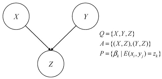
Figure 1.
Basic evidence network diagram.
Using the conditional belief function (CBF) as the parameter model of an evidence network is a very effective way to describe knowledge, which can quantitatively describe the degree of association between the nodes. The expression of the parameters of the evidence network model is provided below.
Definition 5.
Let be the identification frame andbe the basic reliability assignment on. For, the conditional basic belief is defined as
Definition 6.
Letbe the identification frame.is the belief function on, and for, the conditional belief function onis defined as
whererepresents the belief ofgiven.
Definition 7.
Letbe the identification frame.is the plausibility function on, and for, the conditional plausibility function onis defined as
According to the DS evidence theory, there is a correspondence between the BPA, belief function, and plausibility function. Similarly, there is a correlation between the conditional belief function, which can be transformed into each other using the algorithm. The following is the transformation relationship between the conditional BPA, conditional belief function, and conditional plausibility function.
Theorem 1.
Let the identification frames ofandbeand, respectively. If, for any, the conditional belief function ofgivenis
Theorem 2.
Let the identification frames ofandbeand, respectively. If, for any, the conditional plausibility function ofgivenis
Theorem 3.
The following relationships exist between the conditional BPA, conditional belief function, and conditional plausibility function:
3. Structural Modeling of Multi-Level Target Intent Recognition Evidence Network
This section will introduce a target intention recognition method based on evidence network reasoning. Based on data preprocessing, measured data obtained by sensors are used to drive the generation of an evidence network structure and root node belief function, and the evidence network reasoning algorithm based on the conditional belief parameters is then used to solve the non-root node belief function and finally achieve target intention recognition. Figure 2 shows the intent recognition process.
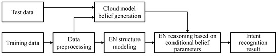
Figure 2.
Process of target intention recognition in evidence network reasoning.
3.1. Evidence Network Structure Modeling
In order to describe the relationship between the nodes of an evidence network more accurately, make the node elements as few as possible, and improve the reasoning efficiency, the correlation between the elements of the network should be considered. The stronger the correlation between the elements, the greater the possibility of a causal relationship between them. Therefore, it is necessary to adopt the evidence network structure modeling method to establish the relationship model between the elements. The structure of evidence network expresses the causal relationship between events. The modeling of evidence network structure expresses the logic of target recognition at the level of qualitative analysis, and it mainly studies the key elements in the system, establishing the relationship between the elements. The structural model of an evidence network mainly includes nodes and edges. Nodes represent research objects, and edges describe the logical relations between nodes. Because the nodes can be determined by the variables in the data set, the edges between the nodes can be mined using the data set.
The traditional evidence network structure modeling is too subjective, so this paper adopts a data-driven evidence network structure modeling method. In order to be able to identify nonlinear functional relations and process uncertain information, a maximum information coefficient (MIC) is introduced in this section to measure the degree of correlation between nodes, determine the existence of edges, and establish the structure of an evidence network. The MIC can capture the correlation between two variables from massive data. Because the MIC is symmetric, that is, , it can only determine if the correlation between the variables is undirected.
Assuming that there are two variables and they have a correlation, a grid can be drawn on the scatter plot corresponding to the two variables, and the relationship between the two can be partitioned. Let represent the finite data set of ordered pairs and , and let the data sample size be N. Given the ordered pairs , the and planes can be divided into multiple units, where such a division is called grid . Let represent the distribution of points in on grid . For fixed , a different grid produces different distributions. The eigenmatrix of data set can be calculated by the following formula:
where, represents the maximum mutual information of grid partition into on data set .
For data set with sample size , the maximum information coefficient can be calculated by the following formula:
where is a function of sample size, usually set as . The degree of dependence of two nodes can be determined by the size of the MIC. If is large, it indicates that node is directly or indirectly connected to node through one or more nodes; if is small, it indicates that the probability of association between node and node is small. When the MIC value between two nodes is large, it does not mean that the two nodes must be directly connected in the evidence network. When a pair of nodes are indirectly connected through multiple nodes, their MIC value will be larger. Therefore, if only the MIC value is used to determine whether nodes are connected, redundant edges will be introduced. An example of producing redundant edges is shown in Figure 3. Figure 3a shows that node and node are indirectly connected through nodes , and , respectively, resulting in a large MIC value. If nodes are directly connected according to the MIC value, the obtained evidence network structure, as shown in Figure 3b, produces redundant edges and is inconsistent with the actual network.
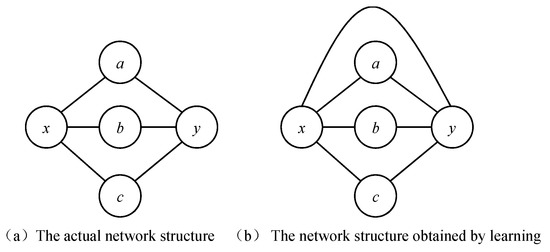
Figure 3.
Example of the causes of redundant edges.
This paper introduces a modified MIC evidence network structure modeling method [36]. The steps are as follows:
Step 1: Create an MIC value list of node , and store MIC values between node and all other nodes in descending order, denoted as .
Step 2: Correct the MIC value and record it as .
where represents the MIC value between node and node and represents the penalty factor. The larger the penalty factor is, the smaller the probability of generating triangle rings in the network, and = 0.1 is preferable. represents a class of nodes in both list and list , and is the number of nodes .
Step 3: Set as the maximum value of in the list, and set as the isolation threshold factor of . If < is satisfied, node is considered as the isolated node.
Step 4: If node and node have undirected edges, the following conditions must be met:
where is the connection threshold factor. The larger is, the stricter the conditions for generating edges and the lower the probability of generating redundant edges.
3.2. Belief Generation Based on a Cloud Model
3.2.1. Gaussian Cloud Model
The cloud model [37] is a mathematical method that can model uncertain data. Three digital features, the expected value , entropy and hyper entropy , are used to represent a concept as a whole. reflects the center of gravity position of the cloud droplet group, reflects the range acceptable by this qualitative concept, that is, the ambiguity, and reflects the cohesion of the uncertainty of all points, that is, the agglomeration of the cloud droplet.
The two-order normal forward cloud model generator is adopted, and its implementation process is described as follows.
Step 1: Generate a normal random number with as the expected value and as the variance.
Step 2: Substitute the measured value to obtain the determination ,
where is the expected value of target characteristic attribute value in the database, is the normal random number obtained in Step 1, and is the measured value of the unknown target.
3.2.2. A Method of Belief Generation Based on Cloud Model
The membership of the target characteristic parameter was set as the mean value of the parameter value. The entropy was times of the standard deviation of the prior value, where the size of reflected the dispersion degree of the estimated noise error. The super entropy was times of the standard deviation of the prior value of the cloud model distribution, and the size of could reflect the randomness. Assuming that the expected value of the characteristic parameter value of an attribute class is and the standard deviation is , the membership degree of the corresponding attribute class is calculated according to the measured data and then converted into the BPA on the attribute.
Step 1: Generate a normal random number with an expected value of and a variance of , ;
Step 2: Substitute the target measurement feature parameter and calculate its membership degree of a certain feature class as:
In this way, the Gaussian cloud model can be used to describe the membership distribution of training samples on each attribute.
Step 3: Construction of composite category attribute model
Target identification needs to rely on multiple attributes, such as speed and height. For the attribute of target speed, membership functions corresponding to high speed, medium speed, and low speed are expressed as , , and , respectively. Different membership functions may intersect, which corresponds to the combination state of categories. If the membership function represents the attribute model that may belong to category or category , its mathematical expression can be described as:
Membership function represents attribute models that may belong to categories , , and , and its mathematical expression can be described as:
Correspondingly, the membership function represents the attribute model that may belong to any category in the identification framework , and its mathematical expression can be described as:
Step 4: Match the test sample with the Gaussian cloud model
Suppose is a proposition in the identification frame and is the value of the test sample on an attribute. Then, the matching degree between the test sample and proposition is defined as:
The size of the value represents the matching degree between the sample and proposition , which depends on the intersection point between the Gaussian cloud model corresponding to proposition and the test sample. can represent either a monad set proposition or a multi-subset proposition. For example, for the target velocity data set, the matching degree between test sample and propositions , , and is defined as:
Step 5: Pignistic probability transformation
Because of the reliability assignment problem of multiple subset propositions, it is impossible to make a decision directly based on the BPA, so the basic belief assignment can be approximated as a probability by using pignistic probability transformation to facilitate the hard decision of evidential reasoning.
Assuming that is the reliability function on the identification frame , represents its pignistic probability distribution, and then corresponding to any element , there is
where is a proposition in the belief function and represents the potential of proposition .
3.3. Construction of Evidence Network Parameters
An evidence network is mainly composed of a network structure and network parameters. Network parameters express quantitative knowledge, that is, the degree of influence from cause to result, and use different forms of belief function to represent the quantitative correlation between nodes. In the process of building an evidence network model for target recognition, network parameters can be in the form of a conditional belief table, and expert knowledge can be included in the conditional belief table, which can reflect the degree of correlation or influence between nodes.
The original DS evidence theory only considers the evidence modeling problem under the same recognition framework. For the relationship between nodes in the evidence network model, it is necessary to consider the evidence representation of two or more variables under different recognition frameworks, namely the joint reliability function model. When the scale of the problem is large and the variable state space is large, the combined explosion problem easily occurs in the joint belief function model. The conditional belief function is an effective way to describe knowledge, and its function is similar to the conditional probability function in Bayesian networks. Compared with the joint belief function model, the conditional belief function model is more direct and easier to understand. In addition, from the perspective of model complexity, the conditional belief function model also has advantages over the joint belief function. Therefore, this paper chooses the conditional belief function as the parameter model of the evidence network.
In order to generate conditional belief, the method based on information entropy is used to determine the conditional belief table. Assume that the characteristic attribute of target intent recognition is , which can be graded by multiple experts. Assume that the evaluation result of an expert is , where represents the th evaluation level, represents its support level, and . If represents the probability at the evaluation grade , a probability distribution defined on can be obtained based on the evaluation results. When determining the conditional belief distribution, entropy can be used to describe the degree of uncertainty in the information. The information entropy of this probability distribution can be calculated and taken as the belief value of multiple subsets. In order to obtain the belief value of the monad set element, the belief value of multiple subsets can be removed and allocated to the monad set in the corresponding proportion:
where represents the number of evaluation levels and represents the number of experts. When the evaluation levels of all experts are different, there is , = = 1. In this case, it means completely unknown. If all expert evaluation results are consistent, such as , and , which means that all reliability is assigned to .
3.4. The Method of Evidence Network Inference
By building an evidence network with the conditional belief as the parameter, and after obtaining the measurement information of some evidence network nodes, it is necessary to estimate the state of unknown nodes through evidence network inference. That is, based on the known network structure model and parameter model, the belief inference algorithm is used to calculate the inference value of nodes of interest. In practice, an evidence network inference for target recognition is used to obtain the key variables of the target recognition system, establish the relationship between them through the evidence network structure model, use the evidence network parameter model to describe the degree of influence between variables, and then deduce the state information of other nodes according to the state information of input variables. In theory, the evidence network inference based on the conditional belief function as the parameter model needs strict mathematical derivation algorithm to achieve effective information transmission. The inference mode can be divided into forward reasoning and reverse reasoning. The inference process includes three main steps: inference initialization, information transfer, and node information update.
Figure 4 shows the evidence network model with belief reliability as the parameter. The node set of the evidence network is , the directed arc set is , the parameter model is and , and the identification framework of is assumed to be and , respectively. Then, the state information of can be obtained from , and conditional belief and ; that is, can be regarded as the function of , , and :
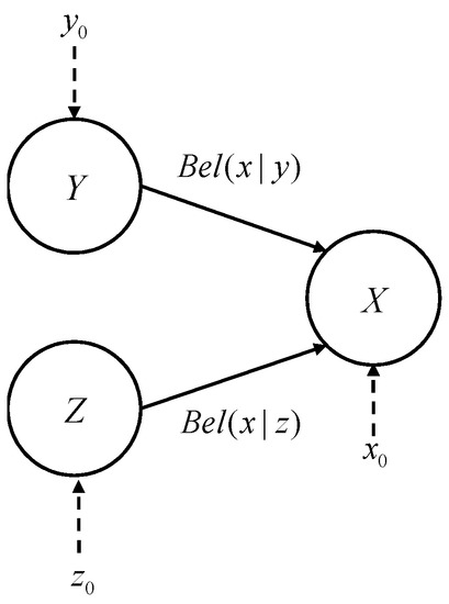
Figure 4.
Evidence network under the conditional belief parameter model.
The solution of function needs to go through several steps, such as information transformation, forward reasoning, and belief synthesis. Information transformation can be processed through the relationship between beliefs. This paper mainly studies the forward reasoning algorithm, proposes a new belief synthesis algorithm, and realizes the evidence network reasoning under the conditional belief parameter model.
Assuming that the identification frames of nodes and are respectively, then for , the conditional basic belief function from to is defined and extended, and the marginalization operation theorems are:
If the belief information on each subset of is known, denoted by , then , and the conditional basic belief can be expressed as
The conditional belief and conditional plausibility function can be expressed as:
For any ,
Through forward reasoning, can be obtained by reasoning from and , and can be obtained by reasoning from and . and need to be synthesized to obtain the final reasoning result of . Dempster’s rule of composition can be adopted for evidence synthesis.
4. The Illustrative Example
This section takes target intention recognition as an example to systematically verify the method proposed above and adopts hierarchical evidence network reasoning, which is divided into three levels of a reasoning and recognition system: state level, action level, and intention level. The data-driven cloud model can generate the belief degree of the feature attributes of the target, which can make full use of the prior information of the known samples of the target, adopt the method based on information entropy to determine the conditional belief table, effectively integrate expert knowledge, and finally realize the intention recognition of the target through evidential reasoning.
4.1. Constructing Evidence Network
Based on the prior knowledge of experts in combination with the MIC algorithm, the correlation between nodes is judged. The evidence network structure modeling is carried out for the target intention recognition, and the dependency and ownership relationship between nodes are obtained. As shown in Figure 5, the target intention can be expressed in a hierarchical way, which is divided into the state layer, action layer, and intention layer. The perceived state describes the state data of the target, indicating the change in the target’s action, including the distance, speed, and other information. Action reasoning describes the action taken by the target and the role it plays, including entity action and electromagnetic action, among which entity action is associated with distance and speed information and electromagnetic action is associated with alarm information. Intentional reasoning describes the inference or estimation of an entity’s intention.
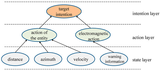
Figure 5.
Evidence network structure of target intent recognition.
Through the previous experiment, it can be seen that after determining the network structure and network parameters, the target intention can be estimated based on the inference method. In the aspect of network structure construction, the algorithm can correctly construct hierarchical evidence network structure by combining expert prior knowledge with the MIC algorithm. Compared with the traditional method that simply relies on expert prior knowledge, the algorithm effectively makes use of the information associated in the data of different attributes. Through experimental verification, the distance, azimuth, and velocity information are associated with the entity action node; warning information is associated with the electromagnetic action, and the entity action node and electromagnetic action node are associated with the target intention node. The whole network structure in Figure 5 conforms to the conditional independence of the data set, and the constructed network structure is reasonable and can meet the requirements of evidential reasoning.
4.2. Cloud Fuzzy Belief Generation
The training samples were selected from the data set to construct its cloud model on various attributes. The remaining samples were used as test samples to test the BPA generation.
According to the recognition framework of target feature attribute as , the , , and of their corresponding training samples are calculated, respectively. For example, under attribute , , , , , and . Similarly, we can obtain the , , and under attribute and , , and under attribute . According to the obtained parameters, the Gaussian cloud model on the target attributes can be constructed as shown in Figure 6.
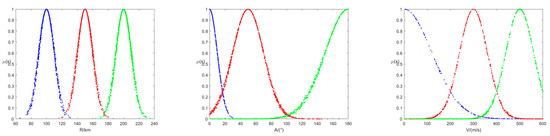
Figure 6.
Gaussian cloud fuzzy membership of target attributes.
On the basis of obtaining the Gaussian cloud model of each attribute of the target, the input sample can be matched with the Gaussian cloud model to obtain the matching degree between the input sample and the characteristic attributes of the target, thus generating the BPA of the test sample.
4.3. Conditional Belief Parameter
Target intent recognition requires input information from sensors, including target distance (), azimuth (), velocity (), warning information (), and output target intent by reasoning through the evidence network. There are specific dependence or influence relationships between nodes in the evidence network. Table 1 describes the framework of variables related to target intent recognition.

Table 1.
Frame description of variables related to target intent recognition.
The evidence network requires a conditional belief table with the state value of each node as the condition to represent the connection strength of causal relationship between nodes. In the process of target intention recognition, a conditional belief table based on the value state of the parent node of a node is also needed to express the strength of the relationship between events or activities. The number of parameters that need to be estimated for the conditional belief exponentially increases with the increase in the number of parent nodes. Therefore, when constructing the conditional belief table, the direct cause of the event should be selected to reduce the number of parameters in the conditional belief table and avoid the combination explosion problem. The conditional belief can be obtained byusing sample learning and expert estimation. When there is not enough sample data, the conditional belief must be estimated, which is a very difficult task. In this paper, the expert knowledge estimation is used to estimate the conditional belief parameters. It is assumed that the conditional belief parameters are formed by combining the knowledge of five experts, and the conditional belief of the entity action node is obtained. The identification frame of entity action node is , and each expert can make an independent evaluation of the three action styles . According to the expert evaluation results, the conditional belief m(PO = F|L, M, H), m(PO = Y|L, M, H), m(PO = P|L, M, H),…, m(PO = FY|L, M, H),…, m(PO = FY|L, M, H) of entity action node is obtained. When five experts provide the m(PO = U|L, M, H), of the evaluation results of , the probability distribution is under the probability distribution, and the physical action node belief distribution can be obtained through the calculation of the following conditions:
The conditional belief parameters of the evidence network of node PO, node EO, and node TI were obtained according to the above methods, as shown in Table 2, Table 3 and Table 4.
Table 2.
Conditional belief parameters of node PO.
Table 3.
Conditional belief parameters of node EO.
Table 4.
Conditional belief parameters of node TI.
In the experiment, the method based on information entropy is used to determine the conditional belief table, which can make full use of the expert knowledge to estimate the conditional belief parameters. As can be seen from Table 2, Table 3 and Table 4, the conditional belief parameters of node PO, node EO, and node TI are given, which can quantitatively reflect the degree of influence of lower level nodes on upper level nodes. For the conditional probability of Bayesian networks, the probability can only be assigned to a single element in the identification frame. However, for the conditional belief data of the evidence network, the conditional parameters of the evidence network can be assigned on the multi-element set. As shown in Table 3, when the conditional parameter W = N, in addition to the assignment of single element EO = H and EO = L of nodes, the conditional reliability parameter m(HL) = 0.3109 can also be assigned to multiple elements EO = HL of nodes, indicating that there is cognitive uncertainty about EO = H, L, and HL under the condition W = N. At this time, a part of the belief is assigned to the recognition frame element HL of the node state. It can be seen that this is a form of multi-element belief allocation that can fully describe inaccurate and incomplete information, reflecting the advantages of evidential reasoning network.
4.4. Evidence Network Reasoning Based on Conditional Belief Parameters
Assume that at a certain moment, the basic belief of target features R, A, V, and W after cloud fuzzy belief processing is
According to the basic belief assignment and conditional basic belief, the corresponding node information is obtained by forward reasoning.
(1) Use the alarm information to conduct electromagnetic action EO reasoning:
After pignistic transformation, the belief degree of the EO single factor is obtained: , .
(2) Reasoning entity action PO according to distance R, azimuth A, and velocity V
After pignistic transformation, the belief degree of the PO single factor is obtained:
(3) Reasoning target intention TI according to entity action PO and electromagnetic action EO
According to the above reasoning and pignistic transformation, it can be concluded that the target intention TI at this time is A, C, and L, respectively, and the reliability is 0.9516, 0.0409, 0.0075, , where it can be concluded that the target intention is A.
The prior belief distribution m(R), m(A), m(V), and m(W) of parent nodes R, A, V, and W can be generated through the cloud model. By using hierarchical evidential reasoning, we can obtain the belief values of different target intentions, and the one with the highest belief value is the target intention. As can be seen from this example, the maximum belief obtained by reasoning is 0.9516, and the corresponding target intention TI is finally determined to be A.
4.5. Comparative Experimental Analysis
4.5.1. Analysis of Accuracy
The evidence network has the ability to deal with uncertain information and incomplete information and can better deal with the noise in the original sensor data. Considering that the current evidence network structure modeling methods are lacking and cannot compare and verify the rationality of the evidence network structure shown in Figure 4 with other modeling methods, the main purpose of this paper is to better verify the effect of an evidence network on target intention recognition, where the network structure is only an intermediate link in the process of target intention recognition. Therefore, this section intends to use the network node and structure model shown in Figure 4 as the benchmark framework for target intent recognition and then select other models for comparative analysis and verification. Considering the similarity between the Bayesian network and evidence network as well as the wide application of the Bayesian network model in target intention recognition, this section introduces the Bayesian network model as the benchmark and measures the effect of the evidence network by comparing the accuracy of target intention recognition results of the two models. In order to compare the effectiveness of the evidence network reasoning method more comprehensively, the evidence network model is compared with the common support vector machine (SVM) model.
The experimental data set mainly includes four attribute information points of the target, which are the distance, azimuth, velocity, and warning information, respectively. The target intention includes A, C, and L. Using the K-fold cross-validation method, the data set was randomly divided into K subsets of almost equal size. A single subset was retained as test data, and the other K-1 subsets were used as training data. The cross-validation was repeated K times, once for each subset. In this experiment, a five-fold cross-validation was used to test the accuracy of intention recognition, and the accuracy of the recognition results is shown in Table 5.
Table 5.
Comparison of target intention recognition accuracy.
As can be seen from Table 5, the accuracy rate of the evidence network is higher than that of the other two models. The SVM model has the lowest accuracy rate, while the accuracy rate of the Bayesian network is between the two models. In the experiment, the accuracy of the evidence network model is higher than that of the Bayesian network model. On the one hand, it can be explained that the evidence network model also has the ability of target intention reasoning and recognition; on the other hand, it also indirectly verifies the accuracy of the established evidence network structure. As a classical target recognition algorithm, SVM has a relatively simple structure, but its parameters have a great impact on the recognition performance, and it is difficult to select the appropriate parameters. In addition, for target intention recognition, SVM directly uses the target attribute data and cannot effectively use the correlation structure information between target attributes such as in the evidence network model. Thus, its recognition accuracy is low.
In order to further study the impact of data size on target intent recognition results, Figure 7 shows the change in recognition accuracy under different training data set sizes. The horizontal axis represents the size of the data, that is, the proportion of the experimental data set (training data and test data) used to the total data. For example, scales = 0.6 indicates that 60% of the data are randomly selected as cross-training data, and the remaining data are used as test data. The vertical axis shows the accuracy of the intention recognition.
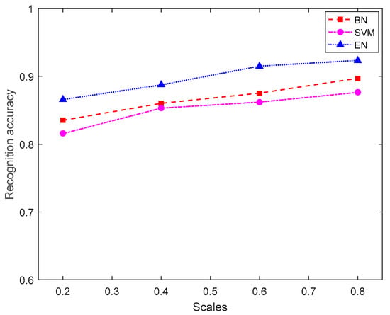
Figure 7.
Comparison of the recognition accuracy of EN, BN, and SVM models with different data scales.
As can be seen from Figure 7, with the increase in training data set size, the curve presents an overall upward trend, indicating that the accuracy of all identification methods presents an overall trend of improvement, and the results are gradually consistent in the region. However, when the scale of training data is small, the identification accuracy of the evidence network is better than the other two types of models. It is found that the identification effect of the evidence network model is obviously better than the SVM model. Compared with the Bayesian network model, the evidence network model also has some advantages as the intention recognition method based on the evidence network model does not need to make accurate probabilistic judgment on uncertain evidence, avoids the loss of uncertain information, and obtains more accurate recognition results.
4.5.2. Analysis of Sensitivity
In order to verify the effectiveness of the algorithm proposed in this paper, noise is added to the feature data of the target, and the noise level is varied according to 10%, 15% and 20% to obtain the belief results of the target intention recognition; the consistency with the known results is compared. Figure 8 shows the recognition belief levels of target intention A, C, and L under three different noise levels. It can be seen that although the noise levels greatly vary, the belief levels corresponding to each element in the framework of target intention identification remain relatively stable, which proves that the proposed intention recognition method is insensitive to noise changes and has good stability and reliability. The proposed method can correctly identify the target intention.
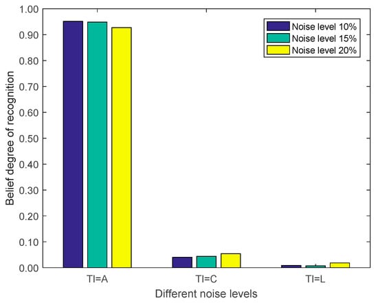
Figure 8.
Target intention recognition belief under different noise levels.
5. Conclusions
Aiming at the practical problems of target recognition such as it being hierarchical and data-driven, this paper proposes a target recognition method based on evidence network reasoning, which realizes the effective recognition of target intention. DS theory can represent probabilistic uncertainty and cognitive uncertainty, and EN provides an expression framework to identify the relationship between nodes of the target. The MIC is used to measure the degree of correlation between nodes, determine the existence of edges, and establish the evidence network structure, which can effectively make up for the shortcomings of the original evidence network structure, which was constructed in a subjective way. The Gaussian cloud model was used to describe the membership distribution of the training samples in each attribute, and the BPA of the target attribute was obtained according to the measurement data of the sensor, which provided the front-end input for the evidence network reasoning. The method based on information entropy is used to determine the conditional reliability table of non-root nodes, which provides a new way to obtain the parameters of the evidence network. Simulation results show that the proposed method can effectively construct a multi-level target intent recognition network model, obtain the target feature belief by using data samples, and realize the target intent recognition by evidential reasoning based on conditional reliability parameters. In the next step, the relative importance of different experts should be considered in the acquisition of the conditional reliability of the evidence network to assign different weights. In addition, due to the different network structures presented by different data sets in practice, research should be carried out on the generation method of the evidence network model based on the characteristics of data sets.
Author Contributions
Conceptualization, H.W. and X.G.; methodology, H.W.; software, H.W., X.G.; validation, H.W., X.Y.; formal analysis, H.W. and X.Y.; investigation, H.W.; resources, H.W. and X.G.; data curation, H.W.; writing—original draft preparation, H.W.; writing—review and editing, X.Y.; visualization, H.W.; supervision, X.Y.; project administration, X.G.; funding acquisition, X.G. All authors have read and agreed to the published version of the manuscript.
Funding
This research was funded by the Youth Foundation of the National Science Foundation of China (grant number 62001503), the Excellent Youth Scholar of the National Defense Science and Technology Foundation of China (grant number 2017-JCJQ-ZQ-003), and the Special Fund for the Taishan Scholar Project (grant number ts 201712072).
Conflicts of Interest
The authors declare that there are no conflict of interest regarding the publication of this article.
References
- Xu, X.; Zheng, J.; Yang, J.B.; Xu, D.L.; Chen, Y.W. Data classification using evidence reasoning rule. Knowl. Based Syst. 2017, 116, 144–151. [Google Scholar] [CrossRef]
- Yang, J.B.; Xu, D.L. Evidential reasoning rule for evidence combination. Artif. Intell. 2013, 205, 1–29. [Google Scholar] [CrossRef]
- Deng, X.; Jiang, W. Dependence assessment in human reliability analysis using an evidential network approach extended by belief rules and uncertainty measures. Ann. Nucl. Energy 2018, 117, 183–193. [Google Scholar] [CrossRef]
- Shenoy, P.P. Binary join trees for computing marginals in the Shenoy-Shafer architecture. Int. J. Approx. Reason. 1997, 17, 239–263. [Google Scholar] [CrossRef]
- Rahman, M.; Islam, M.Z. Missing value imputation using a fuzzy clustering-based EM approach. Knowl. Inf. Syst. 2016, 46, 389–422. [Google Scholar] [CrossRef]
- Mi, J.; Lu, N.; Li, Y.F.; Huang, H.Z.; Bai, L. An evidential network-based hierarchical method for system reliability analysis with common cause failures and mixed uncertainties. Reliab. Eng. Syst. Saf. 2022, 220, 108295. [Google Scholar] [CrossRef]
- Zuo, L.; Xiahou, T.; Liu, Y. Reliability assessment of systems subject to interval-valued probabilistic common cause failure by evidential networks. J. Intell. Fuzzy Syst. 2019, 36, 3711–3723. [Google Scholar] [CrossRef]
- Xiao, F. EFMCDM: Evidential fuzzy multicriteria decision making based on belief entropy. IEEE Trans. Fuzzy Syst. 2019, 28, 1477–1491. [Google Scholar] [CrossRef]
- Chang, L.L.; Zhou, Z.J.; Chen, Y.W.; Liao, T.J.; Hu, Y.; Yang, L.H. Belief rule base structure and parameter joint optimization under disjunctive assumption for nonlinear complex system modeling. IEEE Trans. Syst. Man Cybern. Syst. 2017, 48, 1542–1554. [Google Scholar] [CrossRef]
- Zhou, T.; Chen, M.; Wang, Y.; He, J.; Yang, C. Information entropy-based intention prediction of aerial targets under uncertain and incomplete information. Entropy 2020, 22, 279. [Google Scholar] [CrossRef]
- Simon, C.; Weber, P.; Evsukoff, A. Bayesian networks inference algorithm to implement Dempster Shafer theory in reliability analysis. Reliab. Eng. Syst. Saf. 2008, 93, 950–963. [Google Scholar] [CrossRef]
- Simon, C.; Weber, P. Evidential networks for reliability analysis and performance evaluation of systems with imprecise knowledge. IEEE Trans. Reliab. 2009, 58, 69–87. [Google Scholar] [CrossRef]
- Dempster, A.P. Upper and lower probabilities induced by a multivalued mapping. Ann. Math. Stat. 1967, 38, 325–339. [Google Scholar] [CrossRef]
- Shafer, G. A Mathematical Theory of Evidence; Princeton University Press: Princeton, NJ, USA, 1976; Volume 42. [Google Scholar]
- Machot, F.A.; Mayr, H.C.; Ranasinghe, S. A hybrid reasoning approach for activity recognition based on answer set programming and dempster–shafer theory. In Recent Advances in Nonlinear Dynamics and Synchronization; Springer: Cham, Switzerland, 2018; pp. 303–318. [Google Scholar]
- Jiang, W.; Han, D.; Fan, X.; Duanmu, D. Research on Threat Assessment Based on Dempster–Shafer Evidence Theory. In Green Communications and Networks; Springer: Dordrecht, The Netherlands, 2012; pp. 975–984. [Google Scholar]
- Yang, Y.T.; Yang, J.; Li, J.G. Research on air target tactical intention recognition based on EMEBN. Fire Control Command Control 2022, 47, 163–170. [Google Scholar]
- Xu, J.P.; Zhang, L.F.; Han, D.Q. Air target intention recognition based on fuzzy inference. Command. Inf. Syst. Technol. 2020, 11, 44–48. [Google Scholar]
- Li, Z.W.; Li, S.Q.; Peng, M.Y. Air combat intention recognition method of target based on LSTM improved by attention mechanism. Electron. Opt. Control 2022. Available online: https://kns.cnki.net/kcms/detail/41.1227.TN.20220321.1355.002.html (accessed on 3 January 2023).
- Xue, J.; Zhu, J.; Xiao, J.; Tong, S.; Huang, L. Panoramic convolutional long short-term memory networks for combat intension recognition of aerial targets. IEEE Access 2020, 8, 183312–183323. [Google Scholar] [CrossRef]
- Chen, Y.M.; Li, C.Y. Simulation of target tactical intention recognition based on knowledge map. Comput. Simul. 2019, 36, 1–4. [Google Scholar]
- Kammouh, O.; Gardoni, P.; Cimellaro, G.P. Probabilistic framework to evaluate the resilience of engineering systems using Bayesian and dynamic Bayesian networks. Reliab. Eng. Syst. Saf. 2020, 198, 106813. [Google Scholar] [CrossRef]
- Bougofa, M.; Taleb-Berrouane, M.; Bouafia, A.; Baziz, A.; Kharzi, R.; Bellaouar, A. Dynamic availability analysis using dynamic Bayesian and evidential networks. Process Saf. Environ. Prot. 2021, 153, 486–499. [Google Scholar] [CrossRef]
- Bougofa, M.; Bouafia, A.; Bellaouar, A. Availability Assessment of Complex Systems under Parameter Uncertainty using Dynamic Evidential Networks. Int. J. Perform. Eng. 2020, 16, 510–519. [Google Scholar] [CrossRef]
- Lin, Z.; Xie, J. Research on improved evidence theory based on multi-sensor information fusion. Sci. Rep. 2021, 11, 9267. [Google Scholar] [CrossRef] [PubMed]
- Xu, H.; Smets, P. Reasoning in evidential networks with conditional belief functions. Int. J. Approx. Reason. 1996, 14, 155–185. [Google Scholar] [CrossRef]
- Benavoli, A.; Ristic, B.; Farina, A.; Oxenham, M.; Chisci, L. An approach to threat assessment based on evidential networks. In Proceedings of the 2007 IEEE 10th International Conference on Information Fusion, Quebec, QC, Canada, 9–12 July 2007; pp. 1–8. [Google Scholar]
- Reshef, D.N.; Reshef, Y.A.; Finucane, H.K.; Grossman, S.R.; McVean, G.; Turnbaugh, P.J.; Sabeti, P.C. Detecting novel associations in large data sets. Science 2011, 334, 1518–1524. [Google Scholar] [CrossRef] [PubMed]
- Wang, H.; Deng, X.; Zhang, Z.; Jiang, W. A new failure mode and effects analysis method based on Dempster–Shafer theory by integrating evidential network. IEEE Access 2019, 7, 79579–79591. [Google Scholar] [CrossRef]
- Pourreza, P.; Saberi, M.; Azadeh, A.; Chang, E.; Hussain, O. Health, safety, environment and ergonomic improvement in energy sector using an integrated fuzzy cognitive map–Bayesian network model. Int. J. Fuzzy Syst. 2018, 20, 1346–1356. [Google Scholar] [CrossRef]
- Zuo, L.; Xiahou, T.; Liu, Y. Evidential network-based failure analysis for systems suffering common cause failure and model parameter uncertainty. Proc. Inst. Mech. Eng. Part C J. Mech. Eng. Sci. 2019, 233, 2225–2235. [Google Scholar] [CrossRef]
- Mi, J.; Li, Y.F.; Peng, W.; Huang, H.Z. Reliability analysis of complex multi-state system with common cause failure based on evidential networks. Reliab. Eng. Syst. Saf. 2018, 174, 71–81. [Google Scholar] [CrossRef]
- Qiu, S.; Sallak, M.; Schön, W.; Ming, H.X. A valuation-based system approach for risk assessment of belief rule-based expert systems. Inf. Sci. 2018, 466, 323–336. [Google Scholar] [CrossRef]
- Jiao, L.; Denoeux, T.; Pan, Q. A hybrid belief rule-based classification system based on uncertain training data and expert knowledge. IEEE Trans. Syst. Man Cybern. Syst. 2015, 46, 1711–1723. [Google Scholar] [CrossRef]
- Jiang, J.; Li, X.; Zhou, Z.J.; Xu, D.L.; Chen, Y.W. Weapon system capability assessment under uncertainty based on the evidential reasoning approach. Expert Syst. Appl. 2011, 38, 13773–13784. [Google Scholar] [CrossRef]
- You, Y.; Sun, J.; Ge, B.; Zhao, D.; Jiang, J. A data-driven M2 approach for evidential network structure learning. Knowl. Based Syst. 2020, 187, 104810. [Google Scholar] [CrossRef]
- Wang, G.; Xu, C.; Li, D. Generic normal cloud model. Inf. Sci. 2014, 280, 1–15. [Google Scholar] [CrossRef]
Disclaimer/Publisher’s Note: The statements, opinions and data contained in all publications are solely those of the individual author(s) and contributor(s) and not of MDPI and/or the editor(s). MDPI and/or the editor(s) disclaim responsibility for any injury to people or property resulting from any ideas, methods, instructions or products referred to in the content. |
© 2023 by the authors. Licensee MDPI, Basel, Switzerland. This article is an open access article distributed under the terms and conditions of the Creative Commons Attribution (CC BY) license (https://creativecommons.org/licenses/by/4.0/).