A Novel Process of Parsing Event-Log Activities for Process Mining Based on Information Content

Abstract

Process mining has piqued the interest of researchers and technology manufacturers. Process mining aims to extract information from event activities and their interdependencies from events recorded by some enterprise systems. An enterprise system’s transactions are labeled based on their information content, such as an activity that causes the occurrence of another, the timestamp between events, and the resource from which the transaction originated. This paper describes a novel process of parsing event-log activities based on information content (IC). The information content of attributes, especially activity names, which are used to describe the flow processes of enterprise systems, is grouped hierarchically as hypernyms and hyponyms in a subsume tree. The least common subsume (LCS) values of these activity names are calculated, and the corresponding relatedness values between them are obtained. These values are used to create a fuzzy causal matrix (FCM) for parsing the activities, from which a process mining algorithm is designed to mine the structural and semantic relationships among activities using an enhanced gray wolf optimizer and backpropagation algorithm. The proposed approach is resistant to noisy and incomplete event logs and can be used for process mining to reflect the structure and behavior of event logs.

1. Introduction

The importance of enterprise systems to various business establishments cannot be overemphasized. These systems generate event logs that record all transactions and when they occur. An event is executing a specific action, such as validating a requisition as part of a particular case at an exact time. Consequently, an aggregate of these events, known as an event log, has the recorded actions of the process. Using these event logs, business process mining [1] can uncover new details about an organization’s organizational structure, control, and process discovery. Process mining is handy when extracting these data and understanding the underlying processes. According to Van der Aalst et al. [2], process mining helps practitioners get insight into extracted data from event logs. It focuses on knowledge extraction from data produced and kept in enterprise information systems for process modeling. Process mining has been employed in many industries, including the health industry, to increase the process intelligence of health systems [3].

Business process systems are integral to many organizations’ day-to-day operations because they allow firms to distribute mission-critical information across groups through automated state transitions. Event logs generated during these transitions may help companies find critical data for streamlining their company’s business processes. Process modeling requires using temporal data, such as the timestamps of two events and how often an event has occurred in the past. In a nutshell, process mining aims to gather details about processes from event logs. Each event might have several different attributes, such as an action, a creator, an instance, a timestamp, and many more. A log containing 18 events, 8 activities, 7 creators, and 18 unique timestamps is shown in

Table 1. An example of an event log from [4].

Case_ID	Activity_Name	Resource	Timestamp
Case 1	activity A	Bob	6 January 2021 9:02
Case 2	activity A	Bob	6 January 2021 9:13
Case 3	activity A	Alice	6 January 2021 10:02
Case 3	activity D	Kate	6 January 2021 10:18
Case 1	activity B	Dave	6 January 2021 17:23
Case 1	activity H	Bob	7 January 2021 9:24
Case 2	activity C	Dave	7 January 2021 10:43
Case 4	activity A	Alice	7 January 2021 10:56
Case 2	activity H	Bob	7 January 2021 12:20
Case 3	activity E	Frank	7 January 2021 12:45
Case 3	activity F	Kate	8 January 2021 10:11
Case 4	activity D	Frank	8 January 2021 10:19
Case 3	activity G	Alice	8 January 2021 10:33
Case 3	activity H	Frank	8 January 2021 10:50
Case 4	activity F	Alice	9 January 2021 9:04
Case 4	activity E	Chloe	9 January 2021 9:44
Case 4	activity G	Dave	9 January 2021 11:40
Case 4	activity H	Chloe	9 January 2021 13:32

. Event logs are the first step in the process mining process. There are several perspectives on process mining, including the control-flow-focused, the case, and organizational perspectives [1]. The study focuses on the process perspective. An event log consists of several traces, each representing a sequence of events performed for a particular case, such as an individual order or request. Most foundational process mining techniques treat these traces as sequences of abstract symbols—e.g., a, b, c, d, e, f. In this manner, they make the events abstract, and therefore, uses techniques such as Markov chains, abstraction, evolutionary algorithms, state-based discovery algorithms and language-based region to estimate the control-flow processes of these activities but do not consider the semantics of the data attributes.

Based on empirical evidence, these logs often capture information on the tasks carried out: when they are performed, by whom, and within which circumstance (i.e., process instance). By using the case context in an obvious way, process-discovery algorithms can generate process models that show the process precisely as it happens in the real-life event log. The process perspective, which is our focus, focuses on the control flow, i.e., the ordering of activities. The goal of mining this perspective is to find a good characterization of all possible paths expressed in a Petri net. Process mining researchers, particularly those focusing on the process perspective, have generally concentrated on scanning each event trace in the event log and recording the fundamental ordering relations between activities. These relations provide information on the number of direct task successions. This might result in an object–relation impedance mismatch. However, among these activities, their text is crucial, since it provides a great deal of contextual information and requires a substantial amount of human intelligence.

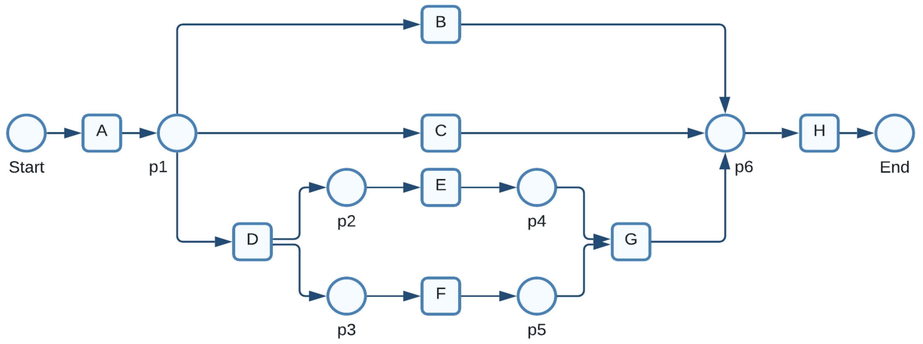
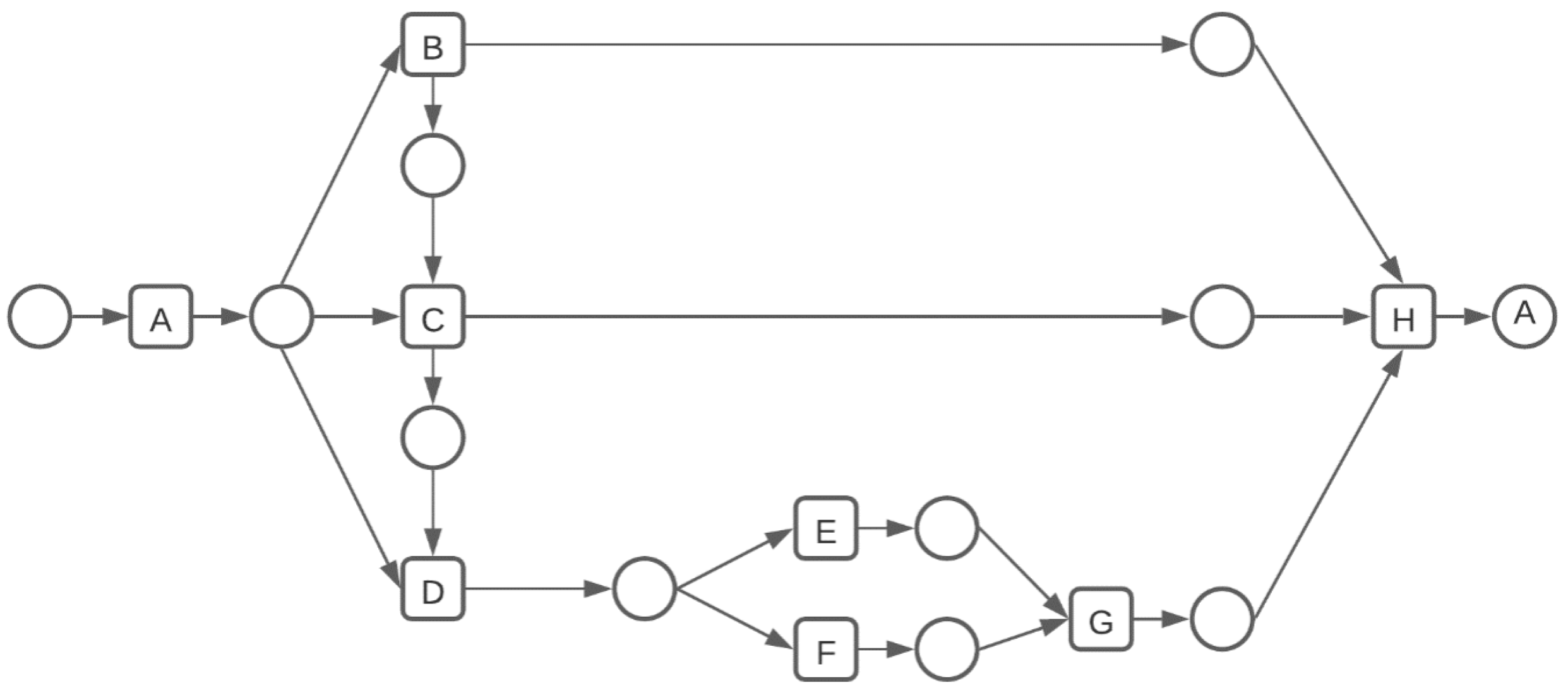
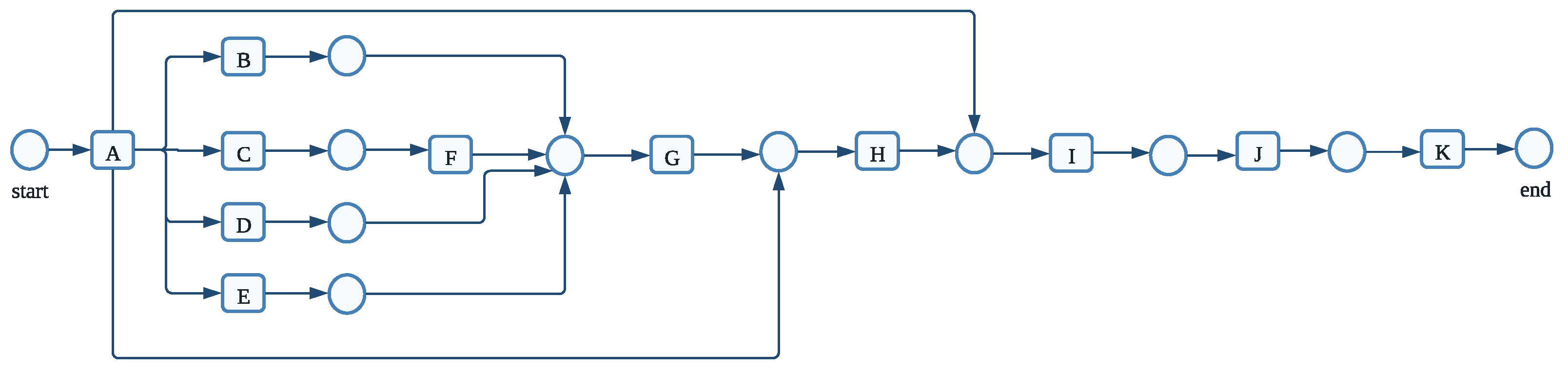
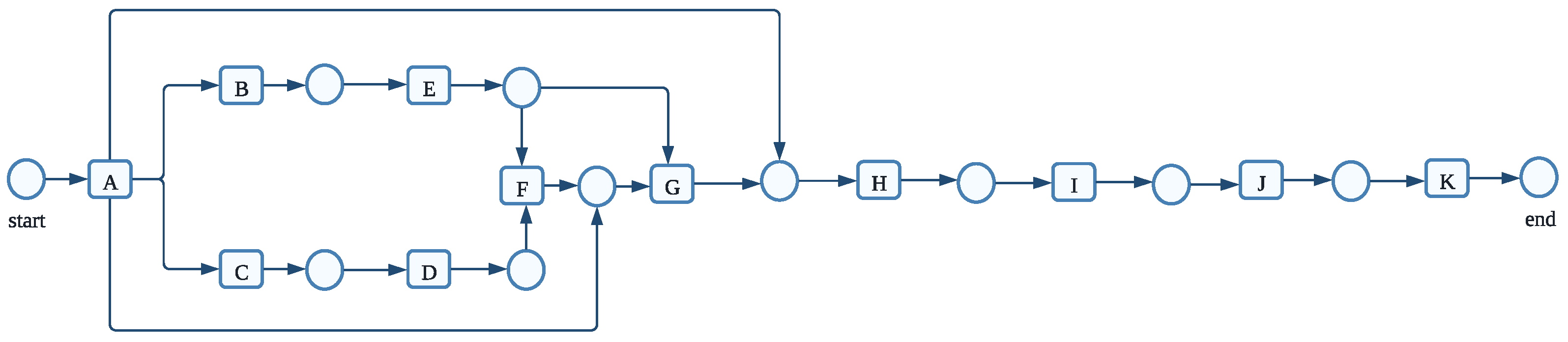
The following cases are observed in Table 1: $\langle A,B,H\rangle$; $\langle A,C,H\rangle$; $\langle A,D,E,F,G,H\rangle$; $\langle A,D,F,E,G,H\rangle$—cases 1 to 4, respectively. We might discover the following details about the process by examining these four cases. The underlying process comprises eight activities $\langle A,B,C,D,E,F,G,H\rangle$. Activity H is always the last activity that must be performed; activity A is always the first to be completed. Activities $\langle B,C,D\rangle$ can be performed after A is finished in any order. H is instantly executed when activities B or C are done, as indicated in cases 1 and 2. Activities E and F can be performed in no particular order after activity D. In this case, both E and F are concurrent. Activities E and F are connected directly by G. Activity H is performed after completing B, C, or G. $P_1$ to $P_6$ are set of places of a Petri net represented by circles As shown in Figure 1, a Petri net (see definition in Section 3.1) may mimic the four event-log scenarios listed in Table 1. A significant field of study that creates an effective tool for text comprehension is the measurement of the semantic relatedness between phrases.

Understanding textual materials more effectively is facilitated by assessing the semantic similarity of terms. This has led to semantic similarity’s use in various tasks, including word-sense disambiguation [5,6], document classification, and clustering [7,8,9]. The taxonomic closeness between words is referred to as semantic similarity or relatedness. Similarity measures calculate a score for semantic evidence obtained in one or more knowledge sources to quantify this closeness. Since the homogenization of web ontology language, numerous developers have built and maintained their systems by augmenting their data vocabularies to precisely describe more constructs from their application domains [10]. For example, there is a relationship among login, logout, confirm payment, checkout, etc. For instance, login has an antonymic relation with log out. Additionally, “checking a receipt” is similar to “confirmation of checking a receipt”, which can be found in an enterprise ticketing system. Since activity names are words used in describing the various components of enterprise systems, this study employs this information-content-based technique to evaluate activity similarity as a function of the information content (IC) that two activities share in a particular log trace. The quantity of information an activity provides when it appears in a trace to another is indicated by its information content (IC). When detected in a discourse, general and abstract entities display less IC than more specific and specialized ones. This paper implements a unique way to parse event activities in an event log by utilizing the information content of the least common submsume of event log attributes. Finally, it provides an algorithm for process mining based on the parsing process using an enhanced gray wolf optimizer with backpropagation.

We recognize that real-world problems are seldom easy to solve. Hence, we employ fuzzy logic to express the similarity values between activities to characterize an event log by considering the information content of the least common subsume between these activities. A fuzzy system is a technique for processing variables that allows for processing several possible truth values using a single variable. It attempts to address problems by using an open, erroneous spectrum of facts and heuristics, resulting in a wide range of reliable findings [11,12,13,14,15]. This generalizes from conventional logic, which holds that all statements have a truth value of one or zero, making it essential for our research. Our method also allows us to define a threshold below which some events may cause the execution of other actions. It is intuitively possible to choose which input and output activities can be executed based on the exact relative weights of activities.

The rest of the paper is presented in the following sections: Section 2 discusses the related work and research gap; Section 3 states the preliminaries; Section 4 and Section 5 present our proposed methodology and a process mining algorithm based on our approach, respectively; Section 6 presents the experimental results. Finally, Section 7 completes the study and provides recommendations for future works.

2. Literature Review

In the past, several process-discovery techniques have been suggested. We go over a few of them in terms of model discovery. Li and Li [16] developed a multi-step process-mining technique for process mining between activities, analyzing a workflow log to accomplish workflow reconstruction using the Markov transition matrix. However, their strategy did not account for sub-processes. Algorithms for discovering genetic process models described in [17,18] use a causal matrix to represent the relationship between activities in an event log. This matrix is represented by 0 s and 1 s, which means activities in a distant relation cannot be represented as activities with a relation. A streamlined process construct tree is a parsing approach to locate block structures in process models, through which soundness can be verified, or an unconstrained model may be transformed into a block-structured one [19]. Joo and Choi [20] defined a stochastic process tree and proposed a tabu search-genetic process mining algorithm for a stochastic process tree. This was done to address the issue of time complexity in genetic algorithms. This is quite similar to our design process in the stochastic process. However, whereas they used a stochastic process tree, we used a levy flight distribution. Interestingly, their approach does not enable the construction of a reliable or accurate model; it simply analyzes or alters an existing model.

The language mining method of Bergenthun et al. [21] pre-structures the input log into new chunks using regular expression; this block-structuring of the log is then employed during discovery to create a fitted, although potentially flawed, process model. The heuristics miner [4] and other frequency-based approaches do not ensure soundness or fitness. Tang et al. [22] proposed a hybrid mining algorithm based on trace clustering population to augment the inefficiencies of genetic process miners. The idea was to simplify the search space, since genetic algorithms inherently do not perform so well on large event logs. Clustering is prone to biases, primarily if the entire population is formed under a biased opinion.

De Leoni, M. et al. [23] proposed a process analysis use case which requires the selection of dependent and independent characteristics and an event filter to describe which events to retain for analysis. They achieved this by incorporating characteristics that are not (yet) available in the event log. These characteristics are added by deriving their values through computations over the event log or from external information sources. Then, the event log is manipulated and enriched with additional characteristics. Finally, based on the correlation analysis results, the traces in an event log are clustered. Song et al. [24] also applied trace clustering for pre-processing event logs. Notably, however, these approaches mainly rely on syntactic information (either control-flow-based or data-flow-based) in the event logs for the pre-processing, leaving a distinct research gap for approaches utilizing semantic information in the pre-processing phase. Additionally, their works concentrate more on event log pre-processing, which is slightly different from ours. Our work seeks to use natural language to generate a process model by using the semantics of the words or phrases used in describing the activity-name event attribute in an event log. Additionally, Sadeghianasl et al. [25] proposed an automatic approach for detecting two types of data quality issues related to activities: synonymous labels (same semantics with different syntax) and polluted labels (same semantics and same label structures) by using activity context, i.e., control-flow, resource, time, and data attributes to detect semantically identical activity labels for detecting frequent imperfect activity labels, just as [26] focuses on event log pre-processing but not the actual process mining itself. Their work tends to correct incorrect labeling of event attributes to enhance the outcome of a process model. Using it to correct incorrect or duplicate labels will further enhance the correctness of our model, since our approach relies on the semantics of the words used in describing processes.

Though clustering-based approaches can increase the simplicity and generalizability of process models, they also lead to a loss of information during the clustering process and introduce biases toward some clusters. Integrating semantic information extracted from the event logs with the mined process models can alleviate this information loss issue. Ideally, a formalized knowledge structure, such as process ontologies, that systematically reflects concepts and their relations could be used as a basis for event-log clustering. However, existing process ontologies are usually generic and lack domain-specificity. Accordingly, lower-level process ontologies require finer granularity and capture domain-specific details through event classes and hierarchical relationships between these classes.

Event log pre-processing before the actual process mining activities is more effective at simplifying the outcomes of process models [26]. Bose et al. [27] have proposed an abstraction-based pre-processing method to deal with loops in mined process models. Abstraction-based approaches usually leverage the premise that all processes are at the same level in an event log, which is not always the case. Additionally, Rebmann, A., and van der Aa, H. [28] identified up to eight semantic components per event. Revealing information on the actions, business objects, and resources recorded in an event log and further categorizing the identified actions and actors allows for a more in-depth analysis of crucial process perspectives. Furthermore, Deokar, A. V., and Tao, J. [29] proposed a computational framework for event log pre-processing, emphasizing event log aggregation. They used phrase-based semantic similarity between normalized event names to aggregate event logs in a hierarchical form.

Overall, existing clustering-based methods used in process mining have changed focus and do not leverage semantics during the pre-processing phase.

Richetti et al. [30] proposed the discovery of declarative process models by mining event logs. It aims to represent flexible or unstructured processes, making them visible to the business and improving their manageability. Although promising, the declarative perspective may still produce models that are hard to understand, due to both their size and the high number of restrictions on the process activities. This work presents an approach to reduce declarative model complexity by aggregating activities according to inclusion and hierarchy semantic relations. The approach was evaluated through a case study with an artificial event log, and its results show complexity reduction in the resulting hierarchical model.

Although numerous researchers have committed efforts to designing efficient algorithms for process mining, an essential difference exists in the parsing of activities. As per available literature, most of the works concentrated on preprocessing event logs for process mining using event-log clustering; others used semantics to correct incorrect attributes labels and to remove duplicates, and finally, semantics of attributes of an event log were used to add invisible attributes that might not have been captured by event log to add more meaning to process mining. Knowing the structural relationship between activities in an event log is not enough. The meaning of the relationship needs to be streamlined, as this will enable process miners to discover how various processes in an enterprise system relate to one another. This will enable terms to be related by natural language processing engines when used for designing process mining algorithms. Thus, we aimed to create a technique that can accurately parse activities in an event log using the semantic relatedness between activities in the event log.

3. Preliminaries

The basic notation used in fuzzy calculus and Petri nets is presented in this section. Petri nets are bipartite-directed graphs for describing concurrent processes [31]. They have places and transitions as their two main types of nodes. The places signify the steps in the process, and transitions indicate actions. The transitions in Petri nets match the events in the event logs. The placement of tokens (black dots) at certain places represents a Petri net’s current state. The firing rule determines the Petri net’s dynamics. If all of a transition’s input places include at least as many tokens as the number of directed arcs that connects them to the transition, following the execution, the transition creates tokens for the output places and deletes tokens from the originating place; thus, a token is eliminated for each input arc from the place to the transition, and on the other hand, a token is created for every output arc.

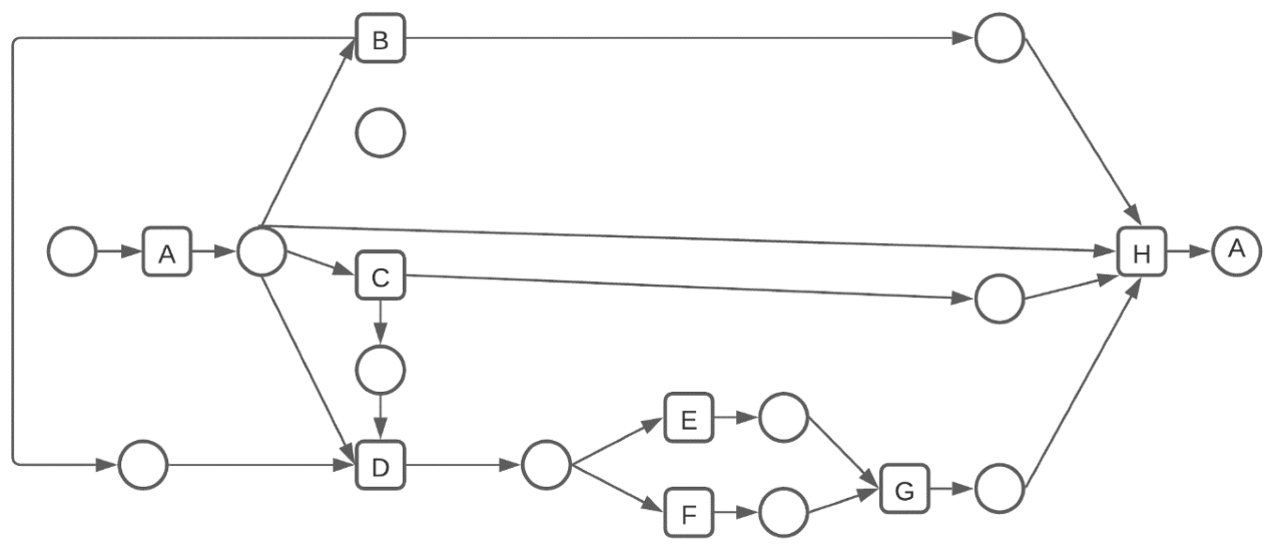
In the initial stage of the procedure for the Petri net shown in Figure 1, there is just one token, Start. This means that in the starting state, only transition A is viable. A removes one token from the initial point and adds one to p1 when it fires. The event log, comprising the four instances (see Table 1), is elegantly represented by the Petri net in Figure 1. Be aware that the Petri net shown in Figure 1 can reproduce each of the four instances, including every observable activity. In this case, the log consists of each possible firing pattern for the Petri net seen in Figure 1. Generally speaking, this is not the case because it is improbable that the log would ever contain all conceivable activity.

3.1. Petri Nets

A Petri net is a four-tuple $N=(P,T,Pre,Post)$, where P is a set of m places represented by circles; T is a set of n transitions represented by bars; $Pre:P\times T\to N$ and $Post:P\times T\to N$ are the pre and post-incidence functions, respectively, that specify the arcs in the net and are represented as matrices in $N^{mxn}$, where $N\ge 0$. For transitions $t\in T$, the set of input places $t=p\in P|Pre(p,t)\ge 0$, and the set of its output places $t^{.}=p\in P|Post(p,t)\ge 0$. Similarly, for places $p\in P$, the set of input transitions $p=t\in T|Pre(t,p)\ge 0$ and the set of its output transitions $p^{.}=t\in T|Post(t,p)\ge 0$.

A marking is a vector $M:P\to N$ that assigns to each place a Petri net, a non-negative integer number of tokens, represented by black dots, and it can also be represented as an m-component vector. $M\left(p\right)$ denotes the marking of place p. A marked Petri net $\langle N,M_0\rangle$ is a net N with an initial marking $M_0$. This is denoted as $R(N,M_0)$—the set of all markings reachable from the initial one. A transition t is enabled at M if $M>=Pre(.,t)$ and may fire, reaching a new marking $M^{\prime }=M+C(.,t)$, where $C=Post-Pre\in {\mathbb{Z}}^{mxn}$.

We denote $M[\sigma \rangle$ as the sequence of transitions enabled at M and $M[\sigma \rangle M^{\prime }$ to denote that the firing of $\sigma$ yields $M^{\prime }$ A marked Petri net is said to be bounded if $\exists K\in N|\forall M\in R(N,M_0)$ and $\forall p\in P,M\left(p\right)\le K$ holds. A Petri net is structurally bounded if, for any $M_0\in N^m$, the marked net $\langle N,M_0\rangle$ is bounded.

3.2. Fuzzy Systems

Fuzzy logic entails a type of logic in which variables’ truth values might be any real integer between 0 and 1. It deals with the idea of partial truth, in which the truth value might vary from totally true to completely false. In contrast, the truth values of variables in Boolean logic can only be the integer values 0 or 1 [32]. Fuzzy logicis mathematically presented as follows [33].

A fuzzy number is a fuzzy set $u:R^1\to I=[0,1]$ such that:

• u is upper semi-continuous.
• $u\left(x\right)=0$ outside some interval $[a,d]$.
• There are real numbers b and c; $a\le b\le c\le d$.
• $u\left(x\right)$ is monotonically increasing on $[a,b]$.
• $u\left(x\right)$ is monotonically decreasing on $[c,d]$.
• $u\left(x\right)=1,b\le \times \le c$.

4. Methodology

4.1. Internal Representation

In our approach, first, we construct a subsume tree of all the activities in the event log based on their information content, i.e., their semantic value and corresponding timestamp values. We then outline our fuzzy causal matrix for parsing individuals. The semantics of fuzzy causal matrix, its generation, and how to generate a process model using an enhanced gray wolf optimizer and back-propagation algorithm are discussed. A process model [1] depicts how activities transition through a business process. It illustrates which behaviors lead directly to the incidence of other behaviors. An activity is routed sequentially if it compares to a specified randomly generated semantic value with the highest value of all the input activities (see Figure 2). Parallel routing happens when an activity allows executing many tasks at once or when several tasks share the same computed similarity values. There are several interdependencies between activities, such as sequential, choice, and parallelism. Given this, a process model must specify which activities lead to the occurrence of others and whether the activities are performed in parallel, sequentially, or through a chosen route. If there are no incoming or departing activities, as seen in Figure 2, these are the starting and ending auxiliaries. We adopt the “start” and “end” to represent this occurrence.

Algorithm 1 is used to obtain the start and end activities. It achieves this by finding the intersection of all the traces in the event log. Indexes 0 and 1 of the obtained intersected activities are set as start and end activities, respectively. We define the intersection as, if $\forall \mathsf{\Gamma }|E{t}_i\in \mathsf{\Gamma }|0\ge i\le max(|{\mathsf{\Gamma }}_i|)$, denoted as $\cap \left(\mathsf{\Gamma }\right)={\cap }_{i=1}^{n}E{t}_i$, where n is the total number of traces.

Algorithm 1: An algorithm to determine start and end activities.

We assume there will likely be two activities in the intersection set. If there are more than two activities, either there is the presence of noise, or the event log is incomplete. We denote $\cap {\left(\mathsf{\Gamma }\right)}_0$ as the starting activity and $\cap {\left(\mathsf{\Gamma }\right)}_1$ as the ending activity. The start activity is used as the hypernym with the assumption that, for each trace, the ordering of the activities from its first activity to the last activity are in a hypernym and hyponymy relations. This enables us to calculate their similarity based on their word sense. From the event log, we can easily recall the timestamp order of the associated sequences of all executed activities. Associative retrieval of events that match the timestamp pattern in each trace would be the next step in building the rest of the subsume tree. The activities that may be retrieved span not just a particular activity’s initial encounter, but also its future encounters and actions.

The tree’s building process is then used to separate the pre- and post-performed operations using the timestamp event property. In Figure 3, the subsume encodes timestamp intervals as the distances between their endpoints in minutes (m), with a directed dotted edge linking each pair. By determining how similar or connected two activities are, the objective is to assign numerical values between $[0,1]$ to them and present them as our fuzzy causal matrix.

4.2. Generating the Fuzzy Causal Matrix

Theoretically, we define a process model as a fuzzy matrix with weighted values in the fuzzy range $[1,0]$ assigned to its rows and columns that show the relationship between activities. A maximum or minimum criterion derived from fuzzy set theory is frequently used to determine the products of fuzzy matrices, which are used to mimic various fuzzy systems. These matrices were initially introduced by Thomason [13].

The fuzzy matrix is $n\times n$ in size, just like any other matrix, where n is the total number of process activities. Fuzzy logic allows for processing many alternative truth values in a single variable. For instance, activity A traverses from itself to the last activity (activity H), and its similarity value is calculated at each activity. It attempts to address problems by using an open, erroneous spectrum of facts and heuristics, resulting in a wide range of reliable findings. This is the strategy we use when presenting our matrix, which describes an event log by considering all pertinent information and applying the best judgment given the input. This generalizes from conventional logic, which holds that all statements have a truth value of one or zero, making it essential for our research. Activity dependencies in our method might have a partial truth value, such as sub-trace $\langle A,C\rangle =0.8$. (see Figure 2). This makes it more likely that the approach will mimic actual circumstances when claims of absolute truth or falsehood are rare.

The relationships’ fuzzy values are used to define the routing architecture. This makes it possible for our system to draw inferences based on data ranges instead of a single discrete data point. The fuzzy causal matrix in

Table 2. Fuzzy causal matrix.

		A	〈A, B〉	〈A ∧ (B ∨ C)〉	D	〈D, E〉	〈E ∨ F〉	〈(B ∨ C) ∧ G〉
$\overrightarrow{\mathrm{yields}}$	A	B	C	D	E	F	G	H
A	1	0.8	0.8	0.8	0.33	0.33	0.28	0.33
B	0.8	1	0.66	0.66	0.28	0.28	0.25	0.85
C	0.8	0.66	1	0.66	0.28	0.28	0.25	0.85
D	0.8	0.66	0.66	1	0.85	0.85	0.28	0.28
E	0.33	0.28	0.28	0.85	1	0.75	0.88	0.25
F	0.33	0.28	0.28	0.85	0.75	1	0.88	0.25
G	0.28	0.25	0.25	0.28	0.88	0.88	1	0.90
H	0.33	0.85	0.85	0.28	0.25	0.25	0.90	1

is created from the least common subsume (LCS) tree. An $8\times 8$ fuzzy causal matrix represents the corresponding event log, since the LCS tree in Figure 1 contains eight activities, $\langle A...H\rangle$. The matrix’s input cell (row, column) specifies how closely two activities are causally related. If the values for (row, column) are 1, then the activities are equal, meaning that activity A equals itself.

All fuzzy values that occur before one in the fuzzy causal matrix are the inputs to their corresponding activities, and the output values are the values after the occurrence of one matrix; i.e., (row, column) = 1 (see Figure 4). Based on the array of fuzzy value entries in the matrix, we may set a threshold value of $(\widehat{S})$ such that values more significant than the threshold and occurring before the activity equals itself (A = A) are viewed as inducing the execution of A. The same goes for (rows, columns) values that occur after the activity equals itself and are more significant than the threshold; these are referred to as output activities.

Definition 1

(Fuzzy Causal Matrix (FCM)). A FCM is a tuple = (A,C,I,O) where

• A is a finite set of activities
• $C\subseteq A\times A$ is the causality relationship (semantic relationship)
• I: A $\to \phi \left(\phi \right(A\left)\right)$ is the input condition function
• O: A $\to \phi \left(\phi \right(A\left)\right)$ is the output condition function

such that

• C = $\exists a\in A|\widehat{S}\langle a_i,a_j\rangle \ge {\rm Y}$, where Υ is a random value
• C = $\exists a\in A|\widehat{S}\langle a_i,a_j\rangle \le {\rm Y}$
• C = $\exists a\in A|\widehat{S}\langle a_i,a_j\rangle =\widehat{S}\langle a_i,a_j\rangle$

A fuzzy causal matrix may be translated to any Petri net that does not have duplicate tasks, does not have more than one place, and has the same input and output tasks. The core premise is that if any one of task A’s output places is an input for task B, then there exists a fuzzy causal relation $\widehat{S}\langle a,b\rangle$ between those two tasks. The output and input places of the activities serve as the foundations for the O and I condition functions. This is an analytical technique of associating Petri nets’ input and output places with the inputs and output functions of the FCM.

Definition 2

(${\Xi }_{N\to FCM}$). Let $N=(P,T,Pre,Post)$ be a Petri net. N can be mapped to ${\Xi }_{N\to FCM}=(A,C,I,O)$. $Pre=P\times T\to N$, $Post=P\times T\to N$, P = places, and T = transitions. $N^{mxn}\ge 0\le N$ is the number of incidence matrices. m = number of place, and n = number of transitions

where

• A = T
• C = $(a_1,a_2)\in T\times T|\widehat{S}(a_1,a_2)\ne \varnothing$
• I $\in T\to \phi \left(\phi \left(T\right)\right)|{\forall }_{t\in T}I\left(t\right)=p\in P|Pre(p,t)$
• O $\in T\to \phi \left(\phi \left(T\right)\right)|{\forall }_{t\in T}O\left(t\right)=t\in T|Post(t,p)$

To construct the Fuzzy Causal Matrix (FCM), we relied on two activities’ significance of the least common subsume (LCS). Activity names in an event log do not take the form of letters in real-world event logs, as indicated in Figure 2; instead, in phrasal form, we depict activity names as letters for simplicity. LCS of two activities $\langle A,B\rangle$, according to Pedersen et al. [34] “Is the most specific concept, which is an ancestor of both A and B”. Similar metrics may be used based on the distance a pair of concepts traverse along a path. The shortest route connecting two tasks is determined by [35], whose scale that is scored by the greatest path length discovered in the $is-a$ hierarchy in which those tasks occur.

The function depth in Algorithm 2 is used to calculate the depth of the least common subsumes of the activities.

Algorithm 2: Function depth(root, x).

We calculate the information content value with Equation (1), then traverse the subsume tree, and calculate the least common subsume value between two activities using Equation (2). Finally, the similarity value between the two activities is then computed. An activity’s depth is just its distance from the root node. The inverse of the shortest path between two activities serves as the measure path’s baseline. The semantic relationship between attributes in an event log tries to capture some of the meaning and structure of log data using abstractions, such as inclusion, aggregation, and association. The following are the formal mathematical representations:

$$IC\left(c\right)=-logp\left(c\right)\cong -log\left(\frac{\frac{|leaves(c)|}{|subsumers(c)|}+1}{maxleaves+1}\right)$$

(1)

Given a pair of activities, $a_i$ and $a_j$, and a set of traces ($\mathsf{\Gamma }$) to which they belong, the selected least common subsume is:

$$LCS(a_i,a_j)=argmax(IC\left(LC{S}_0(a_i,a_j)\right),\forall \mathsf{\Gamma }\exists a|a_i,a_j\in \mathsf{\Gamma }$$

(2)

where $LCS(a_i,a_j)$ is the LCS between $a_i$ and $a_j$

$$depth\left(x\right)=shortestis-apath(root,x)$$

(3)

$$wup=\frac{2\ast depth\left(LCS(a_i,a_j)\right)}{depth\left(a_i\right)+depth\left(a_j\right)}$$

(4)

Algorithm 3 is used to construct a fuzzy causal matrix, as shown in Table 2. The algorithm takes the event log as an input and generates a fuzzy causal matrix (FCM) as an output. The algorithm loops through an event log and creates a list of traces; each trace consists of some activities. The algorithm searches for the trace with the highest number of processes to find the dimensions of the matrix. Usually, event traces do not contain unique activities; some are repeated in different traces. The algorithm only considers such unique values to determine the maximum number of tasks in the log. The findMaxtrace function in the algorithm handls this. The FCM is initialized after the dimension is identified. Algorithm 1 is called, and the start and end activities are initialized. While the dimensionality of the number of activities is not reached, the similarity value between related activities is calculated, and the FCM is populated until the last activity.

Interpretation of FCM and Dependency Measure

Theorem 1.

We made the following assumptions in interpreting the generated FCM. Let FCM be a fuzzy causal matrix.

• $\forall v\in FC{M}_{i,j},\exists D|\stackrel{`}{D},\acute{D}\in D$ where $\stackrel{`}{D}{\left(v\right)}_i$ represents all values of v before 1 in the FCM.
• $\forall v\in FC{M}_{i,j},\exists D|\stackrel{`}{D},\acute{D}\in D$ where $\acute{D}{\left(v\right)}_i$ represents all values of v after 1 in the FCM.
• $\stackrel{`}{D}\left(v\right)$ are the INPUTS of $v_i$ in FCM.
• $\acute{D}\left(v\right)$ are the OUTPUTS of $v_i$ in FCM.
• $\widehat{S}\langle V_i,v_j\rangle$ is the similarity value between $V_i,v_j$.
• If $V_i$ is the start activity, then $v_i$ is the hypernym and $v_j$ is the hyponym and vice versa.
• For $\widehat{S}\langle v_i,v_j\rangle$, initialize a random γ, for which $\widehat{S}\langle v_i,v_j\rangle$ is true.
• For $\acute{D},If\widehat{S}\langle v_i,v_j\rangle \ge \gamma$, then $v_j$ is an output of $v_i$.
• For $\stackrel{`}{D},If\widehat{S}\langle v_i,v_j\rangle \ge \gamma$, then $v_j$ is an input of $v_i$.
• If $\widehat{S}\langle v_i,v_j\rangle =1$, then there is a short loop.
• If $\widehat{S}\langle v_i,v_j\rangle =\widehat{S}\langle v_j,v_i\rangle$, then there is a choice between $\widehat{S}\langle v_i,v_j\rangle$ and $\widehat{S}\langle v_j,v_i\rangle$.
• If $\acute{D}\langle v_i,v_j\rangle =0$, then Start = true.
• If $\stackrel{`}{D}\langle v_i,v_j\rangle =0$, then End = true.

Algorithm 3: Algorithm to generate fuzzy causal matrix (FCM).

Definition 3

(Measuring dependency -ℶ). Let L and T be an event log and a set of activities, respectively. Let $a_1$ and $a_2$ be two activities belonging to T. The measure of dependency $\beth :T\times T\times \ell \to F$ is a function defined as:

$$\begin{array}{c}\beth \langle a,b\rangle =\left\{\begin{array}{c}\widehat{S}\langle a,b,L\rangle \ge \gamma if\exists \stackrel{`}{D}|\stackrel{`}{D}=I\in T|a\ne b\hfill \\ \widehat{S}\langle a,b,L\rangle \ge \gamma if\exists \acute{D}|\acute{D}=O\in T|a\ne b\hfill \\ \widehat{S}\langle a,b,L\rangle =\widehat{S}\langle a,b,L\rangle \mathit{if} a\ne b\hfill \end{array}\right.\end{array}$$

From Table 2 and based on Theorem 1, the relatedness values of 0.8 and 0.66, respectively, among the activities in the sub-trace $\langle A,C\rangle$ and $\langle B,C\rangle$, with respect to activity C, demonstrate the strength (semantics between them) of the association, rather than merely the relationship between the sub traces.

Additionally, row G of activity G in Table 2 contains fuzzy values of 0.88 for both activities, E and F, 0.28 for A, and 0.25 for each of B, C, and D before it equals 1. Activities $\langle A,B,C,D\rangle$ are related to activity G. Still, since their values fall below 0.5, here, assuming 0.5 was chosen as the random similarity threshold, they are disregarded in this situation. Only activities E or F occurrence would result in the execution of activity G—i.e., the occurrence of activity G will only taken place when activities E and F are fired.

Let us consider case 4 in Table 1 $\langle A,D,F,E,G,H\rangle$. Suppose we set a threshold of $\gamma \left(randomvalue\right)\ge 0.2$, where $\gamma$ represents the similarity measure. In that case, a relationship exists between activities A and H, as depicted in Table 2, even though they have a less extreme similarity value of 0.25. In the existing mining algorithms’ causal matrix representation, the relationship between A and H would have been 0. Hence, it would not have been considered in the mining process as there is no relation between activities A and H.

In a typical enterprise system, a user can log in and out almost simultaneously; this needs to be captured in a mined model to depict the behavior of such a user truly. In our approach, lowering the threshold value means more information is contributed to the encoding process, and an overall robust and more representative model is mined. A more intuitive representation of inputs and output values of activities with a threshold of $\gamma \ge 0.5$ is chosen and is presented in Figure 4. The activities in blue are the input activities to activities $\langle B,C,D,E,F,G,H\rangle$ when $\gamma \ge 0.5$, the values in yellow are the output values, and those in green are the input values.

The generation of individuals based on the threshold value and their corresponding Petri nets are shown in

Table 3. Fuzzy causal matrix of individuals of $\gamma$ random values $\ge 0.5$ (individual 1) for the log in Table 1.

Activity	Input	Output
A	$\left\{\right\}$	$\left\{\right\{B,C,D\left\}\right\}$
B	$\left\{\right\{A\left\}\right\}$	$\left\{\right\{C,D,H\left\}\right\}$
C	$\left\{\right\{A\},\{B\left\}\right\}$	$\left\{\right\{D,H\left\}\right\}$
D	$\left\{\right\{A\},\{B,C\left\}\right\}$	$\left\{\right\{E,F\left\}\right\}$
E	$\left\{\right\{D\left\}\right\}$	$\left\{\right\{F,G\left\}\right\}$
F	$\left\{\right\{D\},\{E\left\}\right\}$	$\left\{\right\{G\left\}\right\}$
G	$\left\{\right\{E,F\left\}\right\}$	$\left\{\right\{H\left\}\right\}$
H	$\left\{\right\{B,C\},\{G\left\}\right\}$	$\left\{\right\}$

and 

Table 4. Fuzzy causal matrix of individuals of $\gamma$ random values $\ge 0.28$ (individual 2) for the log in Table 1.

Activity	Input	Output
A	$\left\{\right\}$	$\left\{\right\{B,C,D,E,F,H\left\}\right\}$
B	$\left\{\right\{A\left\}\right\}$	$\left\{\right\{C,D,H\left\}\right\}$
C	$\left\{\right\{A\},\{B\left\}\right\}$	$\left\{\right\{D,H\left\}\right\}$
D	$\left\{\right\{A\},\{B,C\left\}\right\}$	$\left\{\right\{E,F\left\}\right\}$
E	$\left\{\right\{D\left\}\right\}$	$\left\{\right\{F,G\left\}\right\}$
F	$\left\{\right\{D\},\{E\left\}\right\}$	$\left\{\right\{G\left\}\right\}$
G	$\left\{\right\{E,F\left\}\right\}$	$\left\{\right\{H\left\}\right\}$
H	$\left\{\right\{B,C\},\{G\left\}\right\}$	$\left\{\right\}$

and Figure 5 and Figure 6, respectively.

4.3. Parsing Process of Activities

When analyzing an organization’s event log, our technique attempts to identify a process model that best describes the organization’s actual processes. This is achieved by scanning the event log and evaluating the execution relationship between activities. Let us look at trace case 4 $\langle A,D,F,E,G,H\rangle$, and the values presented in the fuzzy causal matrix in Table 2 demonstrate the parsing process. Every trace has a start point and end point. We use these auxiliary components in the marking. As a result, trace case 4 is now $\langle Start,A,D,F,E,G,H,End\rangle$. The parsing process is shown in Figure 7. The left column contains the activities that are being parsed. The right-hand rows indicate which activities’ markings were directly affected by the preceding parsed element, highlighted in yellow. It is evident that parsing an activity impacts how the activities are marked in the resulting fuzzy expression.

The fuzzy values are used to keep the causal relation of each individual marking element. In Figure 7, A is initial element to be parsed. Its input fuzzy value is 0, as there are no incoming activities. It is implied that A is a start activity and can be executed whenever the start is equal to zero. The activity markers are updated following the completion of A. In this instance, A’s output fuzzy values are assigned to the start element’s value of zero. The random value chosen in this parsing process is $\ge 0.5$ (relationship strength), which activates the components with higher $\gamma$ values. Our approach treats OR instances and AND instances differently. For example, when activity D is parsed, elements F and E in the OUTPUT row have the same $\widehat{S}$ value; in this case, activities F and E have an OR relation, and either of them can be executed when D is parsed. Additionally, take note that when D is parsed, A’s marking is impacted, as can be seen in Figure 7; the $\widehat{S}$ value between D and A is 0.8. The fact that activity E and activity G have $\widehat{S}$ values of 0.75 and 0.88, respectively, when activity F is parsed, suggests that E and G are in an AND scenario because of their $\widehat{S}$ values, which are both larger than the $\gamma$ value given in this case.

Additionally, it means that neither the execution of E nor the execution of G is disabled by the other. Thus, it continues in this fashion until all activities are completed. As the end element is the only one indicated with a 0 when the parsing terminates, Figure 7 demonstrates that the individual correctly parsed all activities in Table 2.

Table 5. A fully parsed event log of Table 1 using our approach.

Activity	Input	Output
A	$\left\{\right\}$	$\left\{\right\{B,C,D\left\}\right\}$
B	$\left\{\right\{A\left\}\right\}$	$\left\{\right\{C,D,H\left\}\right\}$
C	$\left\{\right\{A\},\{B\left\}\right\}$	$\left\{\right\{D,H\left\}\right\}$
D	$\left\{\right\{A\},\{B,C\left\}\right\}$	$\left\{\right\{E,F\left\}\right\}$
E	$\left\{\right\{D\left\}\right\}$	$\left\{\right\{F,G\left\}\right\}$
F	$\left\{\right\{D\},\{E\left\}\right\}$	$\left\{\right\{G\left\}\right\}$
G	$\left\{\right\{E,F\left\}\right\}$	$\left\{\right\{H\left\}\right\}$
H	$\left\{\right\{B,C\},\{G\left\}\right\}$	$\left\{\right\}$

shows the output of a successfully encoded individual via our parsing process.

5. Designing a Process Mining Algorithm Using Our Approach

The technique outlined in Section 4 was applied to construct a novel process mining algorithm from a gradient-based and a meta-heuristic algorithm. The powers of the gray wolf optimizer’s global search ability and the backpropagation algorithm’s strong local search ability are combined to profit from the advantages of both approaches while building our mining algorithm. This strategy was chosen to avoid local optimum entrapment, improving the efficiency of discovering optimal process models while also improving the convergence rate. The Levy flight first improves the gray wolf optimizer’s (GWO) global search capability before combining it with back propagation (BP). These techniques are discussed in Section 5.1, Section 5.2 and Section 5.3.

5.1. Gray Wolf Optimization Algorithm

The GWO is a meta-heuristic algorithm based on swarm intelligence that arithmetically replicates gray wolves’ natural leadership mechanism and foraging behavior [36]. They typically live together and go on hunts. Gray wolves’ predatory behavior is modeled using GWO, an adaptive intelligence method based on particle swarm optimization. When it comes to complex function optimization and engineering problems, it works well. The fundamental premise is that gray wolves have a hunting area where they may look for prey. Four divisions of the gray wolf pack may be distinguished based on their hierarchical relationships: alpha, beta, delta, and omega. The alphas are the leaders and are in charge of making hunting decisions. The betas come next, helping the alphas with decision making and other group activities. Omega wolves are at the bottom of the hierarchy and are subservient to alpha, beta, and delta wolves.

The three most essential wolves are $\alpha ,\beta ,$ and $\delta$, who frequently direct the omegas ($\omega$) toward areas with higher hunting potential. We will refer to each alpha, beta, delta, and omega in the search space as a unique process model, and the prey is the model we are trying to reproduce. A population is the limited number of wolves found in any pack at any moment. Each wolf has an internal representation, and the quality of each wolf is assessed using a fitness value calculated using Equation (34) presented in Section 5.4. Observing, encircling, and attacking prey is mathematically characterized by Equations (5) and (6) and results in new places in the search space as the hunt for prey proceeds. We try to mine a process model that reflects the structure and behavior of an event log. Thus, the wolves carry out the hunting process, and the prey, in our case, is the true model we are trying to mine.

$$\overrightarrow{D}=|\overrightarrow{C}.{\overrightarrow{X}}_p\left(t\right)-\overrightarrow{X}\left(t\right)|$$

(5)

$$\overrightarrow{X}(t+1)={\overrightarrow{X}}_p\left(t\right)-\overrightarrow{A}.\overrightarrow{D}$$

(6)

where t shows the current iteration, $\overrightarrow{A}=2.\overrightarrow{a}.{\overrightarrow{r}}_1-\overrightarrow{a}$, $\overrightarrow{C}2.{\overrightarrow{r}}_2$, $\overrightarrow{X}\left(p\right)$ is the position vector for the process model we want to model, and $\overrightarrow{X}$ shows the position vector of a gray wolf (an individual, i.e, the process models generated by our approach). $\overrightarrow{a}$ is a parameter that is linearly decreased from 2 to 0 for ${\overrightarrow{r}}_1$ and ${\overrightarrow{r}}_2$ (random vectors in the range $[0,1]$). Equation (5) indicates the step size of the omega wolf (that is a generated process model with the least fitness measure) towards the specified leader ($\alpha$, $\beta$ and $\delta$); thus, process models with higher fitness values and Equation (6) represent the final position of a process model with the lowest fitness value (the omega $\omega$). From Equations (5) and (6), a gray wolf (an individual), i.e., $(X,Y)$, can update its position to $(X^i,Y^i)$. Henceforth, individuals shall be used interchangeably with process models to describe the process model generated by our approach.

To model the mining process mathematically, we assume that $\alpha$, $\beta$, and $\delta$ individuals have more knowledge about the potential structure and behavior of the true process model we wish to mine. Therefore, they are considered the best candidates, and the omega wolves are forced to update their structural and behavioral constructs according to the best individuals ($\alpha$, $\beta$ and $\delta$). The following equations are used to achieve that.

$${\overrightarrow{D}}_{B\alpha p}=|{\overrightarrow{C}}_1.\frac{\left(\frac{L\left(\sigma \right)}{|\sigma |}x\frac{|Enabled\left(FC{M}_{o,\sigma ,\alpha }\right)\cap Enabled\left(FC{M}_{m,\sigma ,\alpha }\right)|}{|Enabled(FC{M}_{m,\sigma ,\alpha })|}\right)}{L\left(\sigma \right)}-\overrightarrow{X}|$$

(7)

$${\overrightarrow{D}}_{B\beta p}=|{\overrightarrow{C}}_2.\frac{\left(\frac{L\left(\sigma \right)}{|\sigma |}x\frac{|Enabled\left(FC{M}_{o,\sigma ,\beta }\right)\cap Enabled\left(FC{M}_{m,\sigma ,\beta }\right)|}{|Enabled(FC{M}_{m,\sigma ,\beta })|}\right)}{L\left(\sigma \right)}-\overrightarrow{X}|$$

(8)

$${\overrightarrow{D}}_{B\delta p}=|{\overrightarrow{C}}_3.\frac{\left(\frac{L\left(\sigma \right)}{|\sigma |}x\frac{|Enabled\left(FC{M}_{o,\sigma ,\delta }\right)\cap Enabled\left(FC{M}_{m,\sigma ,\delta }\right)|}{|Enabled(FC{M}_{m,\sigma ,\delta })|}\right)}{L\left(\sigma \right)}-\overrightarrow{X}|$$

(9)

$${\overrightarrow{D}}_{B\alpha r}=|{\overrightarrow{C}}_1.\frac{\left(\frac{L\left(\sigma \right)}{|\sigma |}x\frac{|Enabled\left(FC{M}_{o,\sigma ,\alpha }\right)\cap Enabled\left(FC{M}_{m,\sigma ,\alpha }\right)|}{|Enabled(FC{M}_{o,\sigma ,\alpha })|}\right)}{L\left(\sigma \right)}-\overrightarrow{X}|$$

(10)

$${\overrightarrow{D}}_{B\beta r}=|{\overrightarrow{C}}_2.\frac{\left(\frac{L\left(\sigma \right)}{|\sigma |}x\frac{|Enabled\left(FC{M}_{o,\sigma ,\beta }\right)\cap Enabled\left(FC{M}_{m,\sigma ,\beta }\right)|}{|Enabled(FC{M}_{o,\sigma ,\beta })|}\right)}{L\left(\sigma \right)}-\overrightarrow{X}|$$

(11)

$${\overrightarrow{D}}_{B\delta r}=|{\overrightarrow{C}}_3.\frac{\left(\frac{L\left(\sigma \right)}{|\sigma |}x\frac{|Enabled\left(FC{M}_{o,\sigma ,\delta }\right)\cap Enabled\left(FC{M}_{m,\sigma ,\delta }\right)|}{|Enabled(FC{M}_{o,\sigma ,\delta })|}\right)}{L\left(\sigma \right)}-\overrightarrow{X}|$$

(12)

$${\overrightarrow{D}}_{s\alpha p}=|{\overrightarrow{C}}_1.\frac{|C_o\cap C_m|}{|C_m|}-\overrightarrow{X}|$$

(13)

$${\overrightarrow{D}}_{s\alpha r}=|{\overrightarrow{C}}_1.\frac{|C_o\cap C_m|}{|C_o|}-\overrightarrow{X}|$$

(14)

$${\overrightarrow{D}}_{\alpha }={\overrightarrow{D}}_{B,\alpha ,p}+{\overrightarrow{D}}_{B\alpha ,r}+{\overrightarrow{D}}_{s\alpha ,p}+{\overrightarrow{D}}_{s\alpha ,r}$$

(15)

$${\overrightarrow{D}}_{\beta }={\overrightarrow{D}}_{B,\beta ,p}+{\overrightarrow{D}}_{B\beta ,r}+{\overrightarrow{D}}_{s\beta ,p}+{\overrightarrow{D}}_{s\beta ,r}$$

(16)

$${\overrightarrow{D}}_{\delta }={\overrightarrow{D}}_{B,\delta ,p}+{\overrightarrow{D}}_{B\delta ,r}+{\overrightarrow{D}}_{s\delta ,p}+{\overrightarrow{D}}_{s\delta ,r}$$

(17)

$${\overrightarrow{X}}_1=\frac{\left(\frac{L\left(\sigma \right)}{|\sigma |}x\frac{|Enabled\left(FC{M}_{o,\sigma ,\alpha }\right)\cap Enabled\left(FC{M}_{m,\sigma ,\alpha }\right)|}{|Enabled(FC{M}_{m,\sigma ,\alpha })|}\right)}{L\left(\sigma \right)}-{\overrightarrow{A}}_1.(\overrightarrow{D_{\alpha }})$$

(18)

$${\overrightarrow{X}}_2=\frac{\left(\frac{L\left(\sigma \right)}{|\sigma |}x\frac{|Enabled\left(FC{M}_{o,\sigma ,\beta }\right)\cap Enabled\left(FC{M}_{m,\sigma ,\beta }\right)|}{|Enabled(FC{M}_{m,\sigma ,\beta })|}\right)}{L\left(\sigma \right)}-{\overrightarrow{A}}_2.(\overrightarrow{D_{\beta }})$$

(19)

$${\overrightarrow{X}}_3=\frac{\left(\frac{L\left(\sigma \right)}{|\sigma |}x\frac{|Enabled\left(FC{M}_{o,\sigma ,\delta }\right)\cap Enabled\left(FC{M}_{m,\sigma ,\delta }\right)|}{|Enabled(FC{M}_{m,\sigma ,\delta })|}\right)}{L\left(\sigma \right)}-{\overrightarrow{A}}_3.(\overrightarrow{D_{\delta }})$$

(20)

$$\overrightarrow{X}(t+1)=\frac{\overrightarrow{X_1}+\overrightarrow{X_2}+\overrightarrow{X_3}}{3}$$

(21)

where $\overrightarrow{D_{\alpha }}$, $\overrightarrow{D_{\beta }}$, and $\overrightarrow{D_{\delta }}$ are the best behavior and structure for $\alpha$, $\beta$, and $\delta$, respectively. $\overrightarrow{C_1}$, $\overrightarrow{C_2}$, and $\overrightarrow{C_3}$ are random vectors; and $\overrightarrow{X}$ represents the behavior of the potential process model solution. $\overrightarrow{A_1}$, $\overrightarrow{A_2}$, and $\overrightarrow{A_3}$ are randomly distributed vectors. t represents the number of iterations, and Equations (7)–(21) indicate the final nature of the omega wolves.

$L\left(\sigma \right)$ is the log trace, m is our model, and o is the original model. The principle of the GWO algorithm is that the omegas update their next behavior for search according to the positions of alpha, beta, and delta wolves. This makes sure that the individuals with the least fitness measures diverge from each other and converge toward the process model we are trying to mine. When $|A|<1$, the omegas converge towards the desired model, but there is a risk of getting stuck in the local optimum; to prevent it from getting stuck in the local optimum entrapment and emphasizing exploration, $\overrightarrow{A}$ values are considered greater than 1 or small than −1 to force the search agent to diverge from the intended process model.

Again, $\overrightarrow{C}$ is an additional parameter that emphasizes exploration. If $C>1$, it is highlighted; otherwise, it deemphasizes the effect of the process model in defining the distance in Equation (5). It should be noted that $\overrightarrow{A}$ is lowered linearly to encourage exploitation during the iterations. $\overrightarrow{C}$, on the other hand, offers random values to emphasize both exploration and exploitation during optimization. Mirjalili et al. [36] states that it is an effective method for dealing with local optimum stagnation.

5.2. Why Levy Flight?

When the GWO algorithm cannot find the optimal individual after a predetermined number of iterations, levy flight, which follows the levy probability distribution function-based search, is used to enhance the global and local search abilities of the algorithm to prevent it from getting stuck in local optima. This is done by using a random process to come up with random directions and steps that match the levy distribution [37,38]. The levy flight distribution is given as ${L\left(s\right)|s|}^{-1-\beta }$ where $0<\beta \le 2$ is an index. A concise mathematical representation of the levy distribution is presented as follows [39].

$$L(s,\gamma ,\mu )=\left\{\begin{array}{cc}\sqrt{\frac{\gamma }{2\pi }}exp\left[-\frac{\gamma }{2(s-\mu )}\right]\frac{1}{{(s-\mu )}^{\frac{3}{2}}}\hfill & if 0<\mu <\infty \hfill \\ 0\hfill & if s\le 0\hfill \end{array}\right.$$

(22)

where $\mu$ and $\gamma$ are the shift and scale parameters, respectively, and s is the sample distribution. Firstly, a random population is generated, and then the fitness of each individual in that population is determined. Alpha, beta, delta, and omega are initialized in the next stage. After that, the hunting process begins. This process is repeated until there are no further improvements in the outcome. Then, the levy flight is used to continue the search, causing the individuals in the search space to be redistributed. Equations (18)–(20) [40] are then modified to the following.

$$S=\alpha \oplus LEVY\left(\beta \right)$$

(23)

$${\overrightarrow{X}}_1=\frac{\left(\frac{L\left(\sigma \right)}{|\sigma |}x\frac{|Enabled\left(FC{M}_{o,\sigma ,\alpha }\right)\cap Enabled\left(FC{M}_{m,\sigma ,\alpha }\right)|}{|Enabled(FC{M}_{m,\sigma ,\alpha })|}\right)}{L\left(\sigma \right)}+S$$

(24)

$${\overrightarrow{X}}_2=\frac{\left(\frac{L\left(\sigma \right)}{|\sigma |}x\frac{|Enabled\left(FC{M}_{o,\sigma ,\beta }\right)\cap Enabled\left(FC{M}_{m,\sigma ,\beta }\right)|}{|Enabled(FC{M}_{m,\sigma ,\beta })|}\right)}{L\left(\sigma \right)}+S$$

(25)

$${\overrightarrow{X}}_3=\frac{\left(\frac{L\left(\sigma \right)}{|\sigma |}x\frac{|Enabled\left(FC{M}_{o,\sigma ,\delta }\right)\cap Enabled\left(FC{M}_{m,\sigma ,\delta }\right)|}{|Enabled(FC{M}_{m,\sigma ,\delta })|}\right)}{L\left(\sigma \right)}+S$$

(26)

$$\overrightarrow{X}(t+1)=\frac{\overrightarrow{X_1}+\overrightarrow{X_2}+\overrightarrow{X_3}}{3}$$

(27)

where ⊕ is an entry-wise multiplication product and $\alpha$ is a random number in Equation (23). As can be seen in Equations (24)–(26), the behavior and structure of the individuals are added to S. S is calculated by the method defined by [40] as follows:

$$s=0.01\ast \frac{u}{v^{\frac{1}{\beta }}}\ast (X-X_{\alpha })$$

(28)

where v and u are random numbers generated by a normal distribution:

$$u\sim N(0,{\mu }_u^2),v\sim N(0,{\mu }_v^2),$$

(29)

with

$${\mu }_u={\left\{\frac{\tau (1+\beta )sin\frac{\pi \beta }{2}}{\tau \left[\left(\frac{1+\beta }{2}\right)\right]\beta 2^{\frac{\beta -1}{2}}}\right\}}^{\frac{1}{\beta }},{\mu }_v=1$$

(30)

where $\tau$ is the standard gamma function. For each individual as the best candidate, a random number $\beta$ is generated between 0 and 2. The smaller the value of $\beta$, the higher the jumps, and the larger the values of $\beta$, the lower the jumps. It means higher values of $\beta$ will cause jumps to unexplored search space, and as a consequence, prevent it from getting stuck in local optima. On the other hand, smaller values of $\beta$ trigger new search spaces to be considered near the obtained solutions.

The gray wolf algorithm has a tremendous global search ability but a low convergence rate. To deal with this flaw, the BP algorithm, which has strong local and poor global search capabilities, is paired with the gray wolf to profit from the advantages of both approaches while constructing our mining algorithm. Consequently, the BP algorithm refines the GWO results to generate more accurate results, enhancing the efficiency of our proposed technique in discovering optimum models and accelerating the rate of convergence.

5.3. Backpropagation

We assume our generated process model to be a neural network, and the input activities are the inputs to the network. The activity directly above an element with a higher value of $\mathsf{\Gamma }$ than it is an input to that activity. Finally, activities with lower values of Ŝ are the hidden nodes of the network. There are as many events in an event log as there are nodes in the input layer, and vice versa for the output layer. However, depending on the number of activities and their relationships in an event log’s trace, the number of hidden activities might vary. We take i as the number of activities in the input layer, h as the number of activities in the hidden layer, and o as the number of activities in the output layer. It can therefore be calculated as:

$$L_k=f\left({\mathsf{\Sigma }}_{m=1}^h(w_{nm}f\left({\mathsf{\Sigma }}_{i=1}^i(w_{nm}{x}_l+{\theta }_{wm})\right)+{\theta }_{wm})\right)$$

(31)

where $L_k$ is the output of the $n^{t}h$ node in the output layer of the individual; $x_l$ is the input of the $l^{t}h$ node in the input layer; $w_{nm}$ is the semantic value between two activities; $\widehat{S}$ and ${\theta }_{wm}$ represent bias terms of the sigmoid function f of nodes m in layer h of activities and nodes n in the output layer. We calculate the transfer function f using the sigmoid function as follows:

$$f\left(x\right)=Sigmoid\left(x\right)=\frac{1}{1+exp(-1)}$$

(32)

The semantic value between activities and the bias term of each trace constitutes the causal relationship between activities. We can calculate the error of obtaining the required process model by calculating the loss function. This is used to measure the discrepancy between the target and generated models. Equation (33) is used to calculate the loss function as follows:

$$MSE=1/n{\mathsf{\Sigma }}_{i=1}^n{\mathsf{\Sigma }}_{j=1}^k{(y_i-\widehat{y_i})}^2$$

(33)

where k shows the number of tasks in the log; the lower the value difference, the closer the mined process model will be to the actual model.

5.4. Fitness Calculation

Process mining aims to discover a process model from an event log. The mined process model should provide helpful insight into the log’s behavioral characteristics. In other words, from a behavioral and structural standpoint, the mined process model should be accurate and comprehensive. A model is complete when it can analyze or replicate every event trace in the log and is precise when it cannot parse more than the traces in the log [3]. Models that can parse all event traces may provide an additional activity that does not belong in the log, making it crucial that the mined model also be exact. As a result, each individual’s fitness is determined, and the results are $X\alpha$ as the model with the lowest cost, $X\beta$ as the model with the second-lowest cost, and $X\delta$ as the model with the third-lowest cost.

The fitness of the generated process models assesses how effectively an individual represents the behavior in an event log, new solutions are created, and their fitness is calculated to generate new process models. We determine the fitness of each trace and aggregate them. Our fitness measure, the “completeness” metric, is based on how individuals parse event traces. The ideal individual or model should have a fitness score of one for a noise-free log. The following equation is used to calculate the fitness at the trace level of an event log.

$$fitness(\sigma ,N)=0.5\left(1-\frac{m}{c}\right)+0.5\left(1-\frac{r}{p}\right)$$

(34)

where m is the number of missing tokens, c the number of tokens consumed, r is the tokens left after it reaches an output place, and p is the number of tokens produced. From Section 3, we learned that an event log contains several traces; hence, we aggregate all cost functions of all the traces. The following is the combined fitness function of a log.

$$f(L,N)=\frac{1}{2}\left(1-\frac{{\mathsf{\Sigma }}_{\sigma \in L}L\left(\sigma \right)\ast m_{N,\sigma }}{{\mathsf{\Sigma }}_{\sigma \in L}L\left(\sigma \right)\ast c_{N,\sigma }}\right)+\frac{1}{2}\left(1-\frac{{\mathsf{\Sigma }}_{\sigma \in L}L\left(\sigma \right)\ast r_{N,\sigma }}{{\mathsf{\Sigma }}_{\sigma \in L}L\left(\sigma \right)\ast p_{N,\sigma }}\right)$$

(35)

where $L\left(\sigma \right)$ is the number of times the trace occurred in the log.

5.5. Analysis Metrics

Medeiros et al. [17] defined evaluating metrics to evaluate mined models on completeness and precision. To check for completeness, a partial function measure is defined as.

$$P{F}_c(L,FCM)=\frac{allParsedActivities(L,FCM)-punishment}{numActivitiesLog\left(L\right)}$$

(36)

where

$$punishment=\frac{\frac{e(L,FCM)}{n\left(Log\right)-f(L,FCM)+g(L,FCM)}}{n\left(L\right)-h(L,FCM)+1}$$

(37)

where $allParsedActivities(L,FCM)$ is the total number of successful parsed activities in the event log, $allMissiongTokens(L,FCM)$

Indicates all missing tokens in a trace, where n = number of traces in the log, e = all missing tokens, f = number of traces missing tokens, g = all extra tokens left behind, and h = number of extra tokens that are left behind. g(L,FCM) denotes unconsumed tokens after the parsing of activities has completed, in addition to tokens at the end place minus 1, and n(L) represents the number of traces in L. (L,FCM) and h(L,FCM), respectively, represent the numbers of traces with missing tokens and the remaining tokens after the parsing process has completed.

This metric provides more specific information on how well a certain process model fits a particular log. It accurately determines how much other behavior an individual permits. Medeiros et al. [17] checked the number of activated visible tasks. Others who allow extra behavior typically have more enabled tasks than those who do not. The primary purpose is to benefit individuals with fewer enabled tasks while parsing the log. Precision is defined using the following equation.

$$P{F}_p(L,FCM,FCM\left[\right])=\frac{allEA(L,FCM)}{max\left(allEA\right(L,FCM\left[\right])}$$

(38)

where $allEA(L,FCM)$ denotes all enabled activities during the parsing process of log L, $allEA(L,FCM[\left]\right)$ applies enabled activities to each activity in the matrix, and (allEA(L,FCM[]) returns the maximum value of the number of enabled activities in the given population (FCM[]) while parsing the log (L). Therefore, the complete fitness function for our evaluation combines both $P{F}_c$ and $P{F}_p$, such that, for a none empty log (L), the fuzzy causal matrix, a bag of causal matrices FCM[], and a real number k, F(L,FCM,FCM[]) = $P{F}_c(L,FCM)-k\ast P{F}_p(L,FCM,FCM\left[\right])$, where k punishes an individual for extra behavior.

We established two measures, behavioral precision and behavioral recall, because we needed to compare the behavior of the original model with that of the mined model. Both are based on the original model and the mined model’s parsing of an event log. These metrics function by comparing the number of tasks enabled in the original model and the mined model for the continuous semantics parsing of every task in every process instance of the event log. The models’ behaviors are increasingly similar with the more enabled tasks they share. The behavioral precision determines how much deviation from the mined model the original model permits, in contrast to the behavioral recall. Both metrics also include the frequency with which a trace appears in the log. As deviations belonging to uncommon pathways are less significant than deviations related to normal behavior, this is particularly essential when working with logs in which specific paths are more prevalent than others. The more similar $B_P$ and $B_R$ behaviors are to one, the closer their behaviors are. $B_P$ is defined as [17].

$$B_P(L,FC{M}_o,FC{M}_m)=\frac{{\mathsf{\Sigma }}_{\sigma \in L}\left(\frac{L\left(\sigma \right)}{|\sigma |}x{\mathsf{\Sigma }}_{i=1}^{|\sigma |}\frac{|E\left(FC{M}_{o,\sigma ,i}\right)\cap E\left(FC{M}_{m,\sigma ,i}\right)|}{|E(FC{M}_{m,\sigma ,i})|}\right)}{{\mathsf{\Sigma }}_{\sigma \in L}L\left(\sigma \right)}$$

(39)

where $E(FCM,\sigma ,i$) returns the enabled tasks at the fuzzy causal matrix before the parsing of the activity at position i in the trace $\sigma$ and behavioral recall as:

$$B_R(L,FC{M}_o,FC{M}_m)=\frac{{\mathsf{\Sigma }}_{\sigma \in L}\left(\frac{L\left(\sigma \right)}{|\sigma |}x{\mathsf{\Sigma }}_{i=1}^{|\sigma |}\frac{|E\left(FC{M}_{o,\sigma ,i}\right)\cap E\left(FC{M}_{m,\sigma ,i}\right)|}{|E(FC{M}_{o,\sigma ,i})|}\right)}{{\mathsf{\Sigma }}_{\sigma \in L}L\left(\sigma \right)}$$

(40)

Additionally, we used the following equations to assess the structural similarity of the original and the mined models. This metric checks the number of causal relations shared by the original and the mined model. The higher the number of causal relationships that exist between them, the more similar their structures are. There are two metrics, structural precision and structural recall. The former assesses the difference in causal relations between the mined and the original model, and the latter evaluates otherwise. Structural precision is defined mathematically as.

$$S_P=\frac{|C_o\cap C_m|}{|C_m|}$$

(41)

$$S_P=\frac{|C_o\cap C_m|}{|C_o|}$$

(42)

$P{F}_c$, $P{F}_p$, $B_P$, $B_R$, $S_P$, and $S_R$ are the metrics used to analyze the mined models in this paper.

5.6. Pseudocode of the Algorithm

After generating the fuzzy causal matrix, we use it to construct our mining algorithm. The pseudocode of the mining algorithm is presented in Algorithm  4.

Algorithm 4: Pseudocode of the mining algorithm.

6. Experimental Results

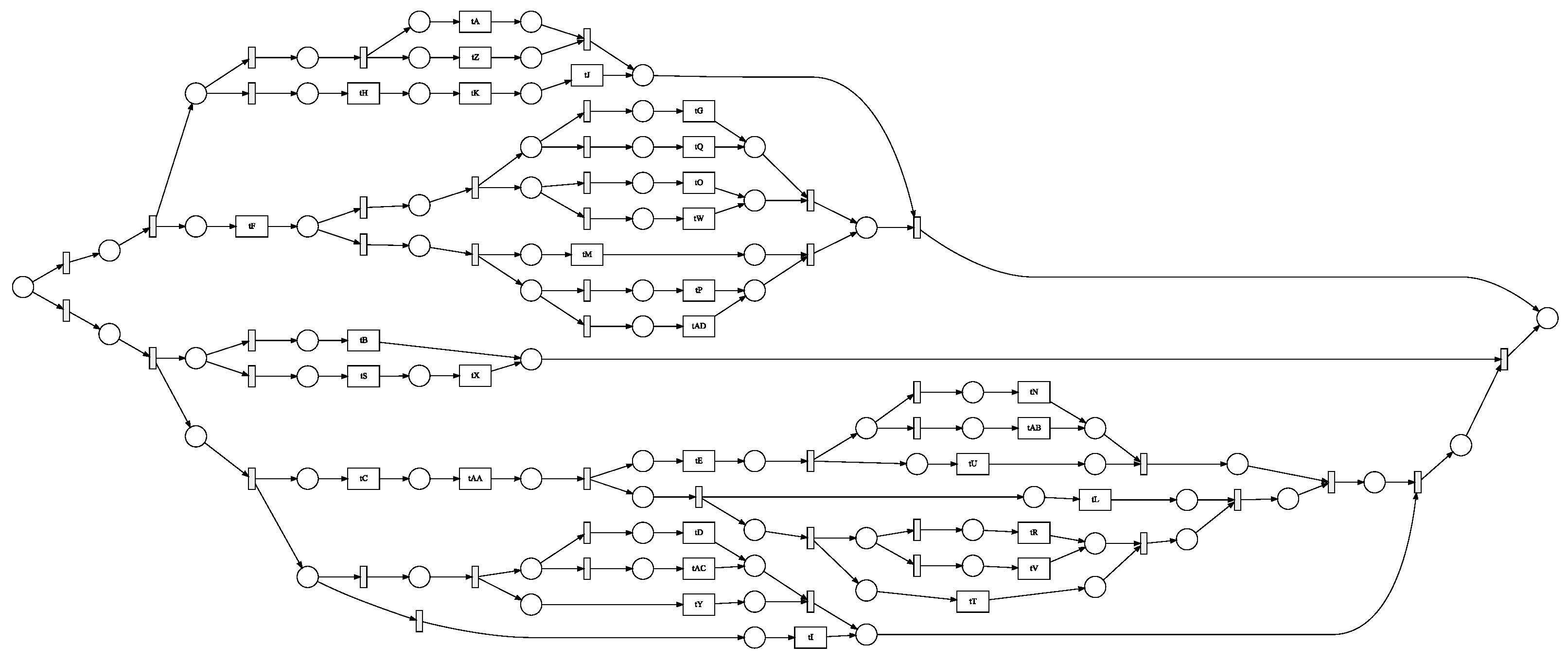
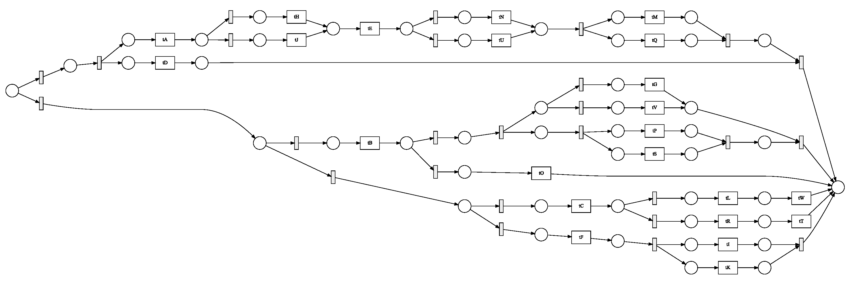
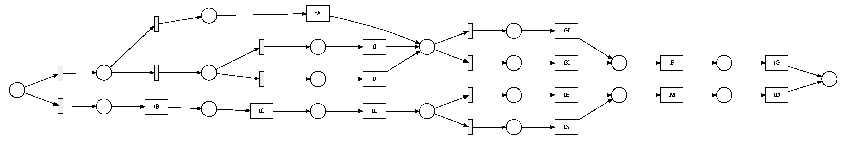
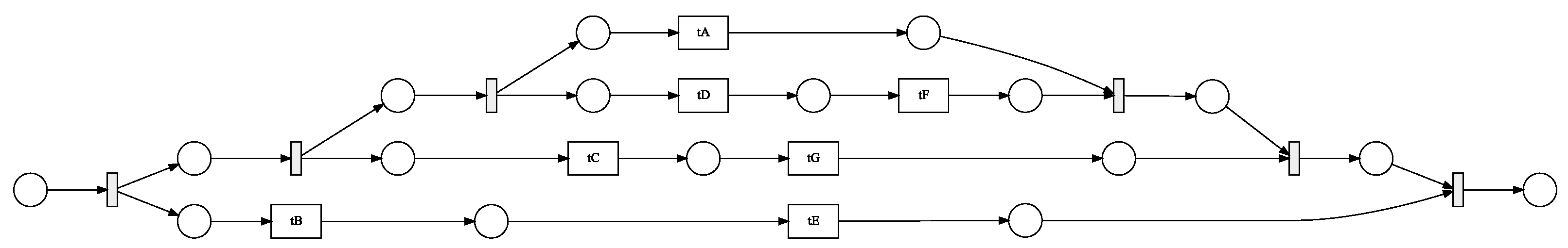
We employed four distinct process models with 7, 14, 24, and 30 activities to test our enhanced gray wolf optimizer (GWO) with backpropagation for process mining. We tested the effects of the basic gray wolf optimizer (GWO), an enhanced gray wolf optimizer (EGWO), and the enhanced gray wolf optimizer with backpropagation (EGWO + BP) on the proposed parsing of event logs. These models were created artificially using the ProM6.10 for process mining plugin (to generate a block-structured stochastic Petri net). They include concurrency, loops, and sequences. Figure 8, Figure 9, Figure 10 and Figure 11 each describe one of these nets. We employed six distinct forms of noise to examine how our proposed method deals with noise-free and noisy event logs. The types of noise examined include exchanged activities, mixed noise, missing head, missing activity, missing tail, and a missing body. These noise types behave as follows, assuming an event trace $\sigma |{\sigma }_1,{\sigma }_2,...,{\sigma }_n\in \sigma$.

Missing head, tail, and body noise involves randomly removing sub-traces of activities in the head, tail, and body of $\sigma$. The head goes from ${\sigma }_1$ to ${\sigma }_n/3$. The body goes from $\sigma (n/3)+1$ to $\sigma (2n/3)$, and the tail goes from $\sigma (2n/3)+1$. Missing activity randomly removes an activity from the trace. Two activities are exchanged in the exchanged activity noise type. The mixed noise type comprises a mixture of the five above mentioned noise types. Real-world logs frequently include a variety of noise. However, the distinction between the noise types enables us to more accurately evaluate how the various noise types impact the algorithms used in generating a process model from event logs. We produced logs with 5%, 10%, and 15% noise for each category of noise. Therefore, we had 18 noisy logs in each process model in our experiments.

We tested our methodology with noise-free logs from process models which should provide similar results. We initialized the number of activities per generated process model; the dimensions were set to $n\times n$, depending on the number of activities in the corresponding process model. We set the lower and upper bounds to −10 and 10, respectively. The population had 300 individuals and was iterated a maximum number (max_iter) of 150 times. After several iterations, the best models with suitable fitness measures were obtained. Each event log consists of 500 traces. For each log, the three algorithms ran five tests with randomized seeds. As we know, for the model used to generate the event logs, we expect the various GWO techniques to yield the same model during experimentation. In a more realistic setting, though, the underlying model is unknown, and we will have to search for it. The only realistic answer seems to be the definition of a suitable algorithm that will provide us with the best fitness metric. The gray wolf optimizer (GWO) was tested alone without levy flight and with Levy flight (EGWO), and the enhanced GWO with backpropagation (EGWO + BP) was tested. It is possible to calculate a fitness index from each of these algorithms. One way we have found to quantify the efficacy of our algorithm in this experimental situation is by tallying the frequency with which the GWO search yields the process model employed while generating the noise-free event logs. This metric will be used even if there is extra noise in the event log.

Let us first have a look at the results for the noise-free logs. As shown in Figure 12, the algorithm works for noise-free logs. For the three scenarios w.r.t. to fitness, the smaller the net, the more frequently the gray wolf algorithm without enhancement finds the desired process model. Additionally, the enhanced version performs slightly better than the GWO. This could be attributed to the dynamic position updating of the best solutions by incorporating the levy flight distribution, which is stochastic, since GWO disregards the positional interaction information about the best three solutions. For process models that contain more activities, the enhanced gray wolf with backpropagation produced better process models than both the GWO alone and its enhanced version (EGWO). This could be attributed to the stagnation of the GWO in local optima when the search space is relatively large.

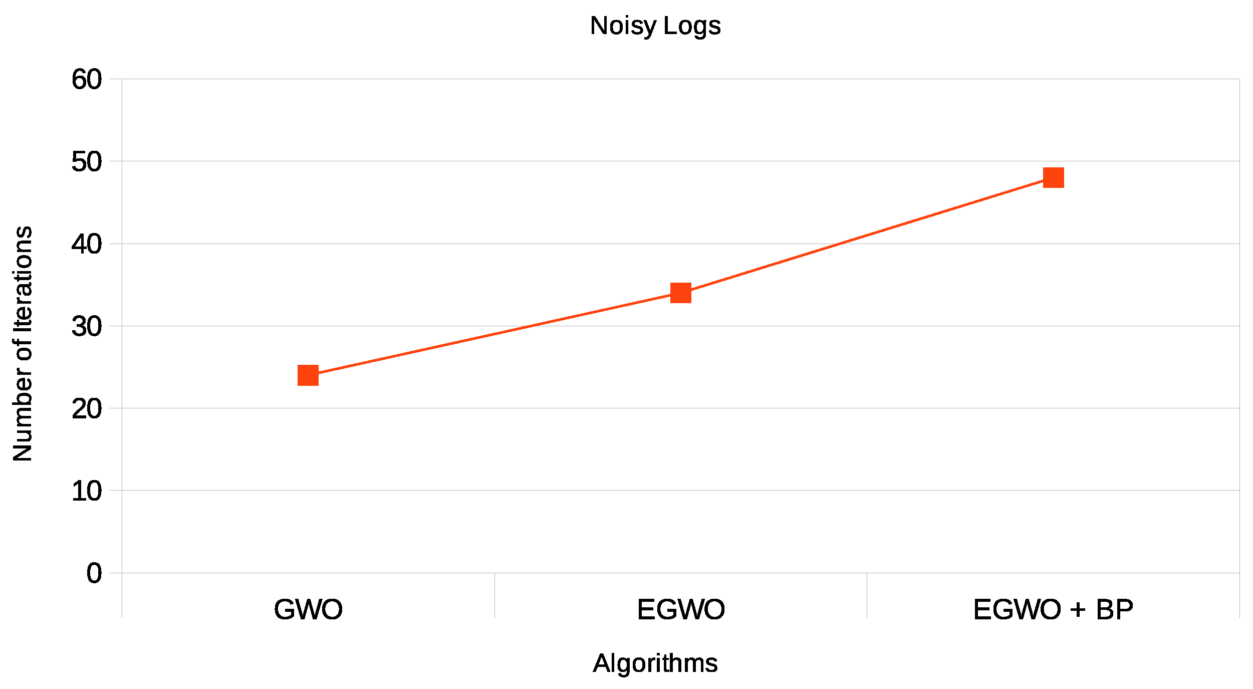
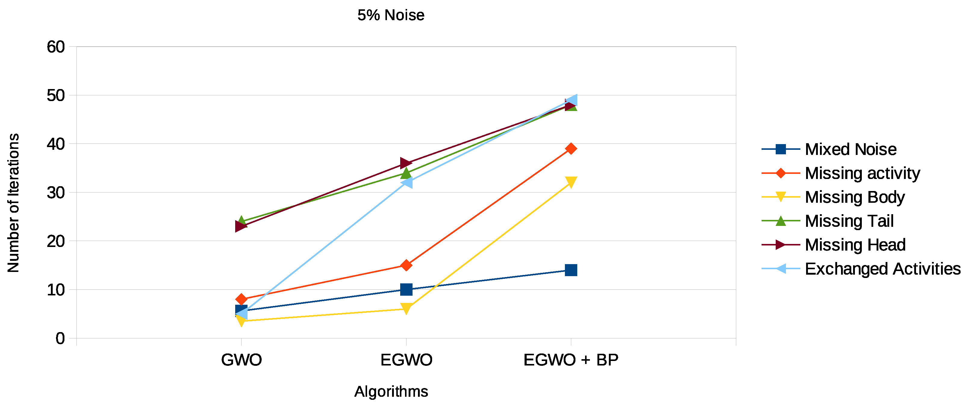
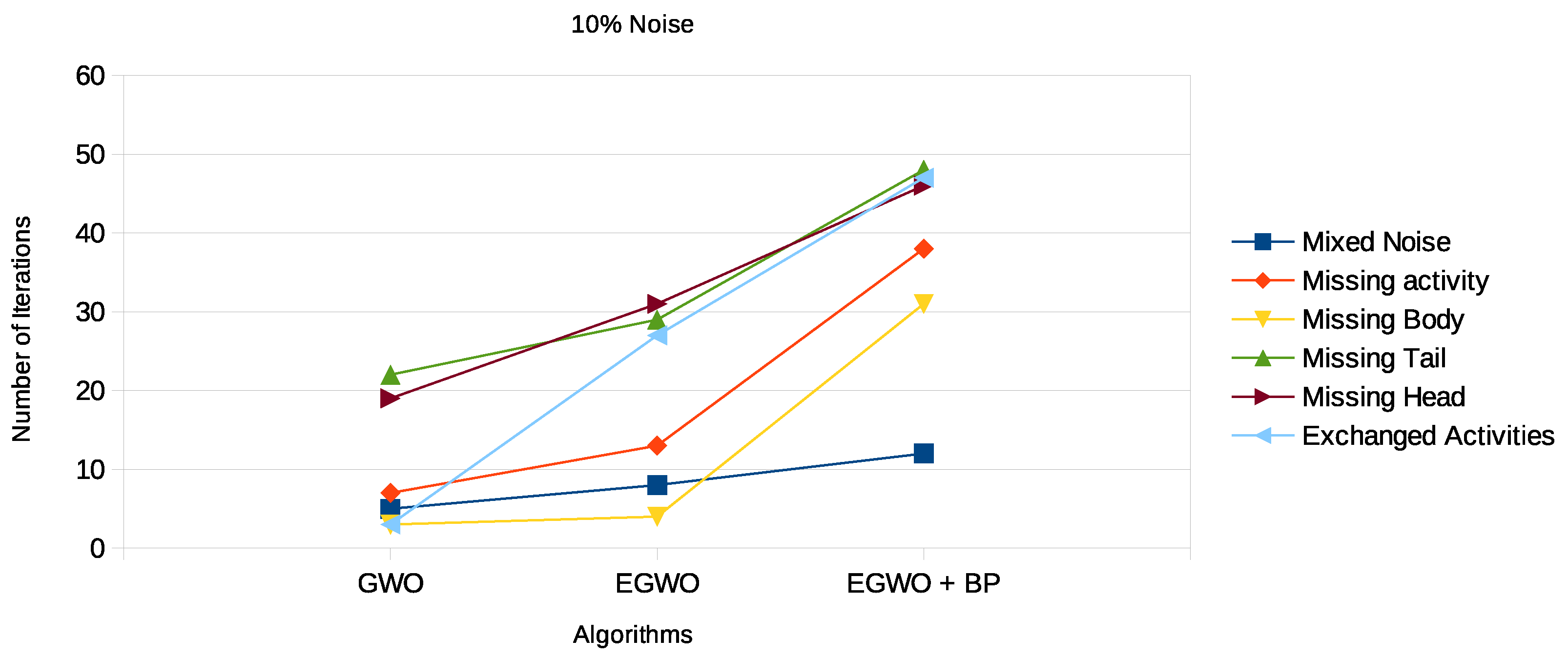
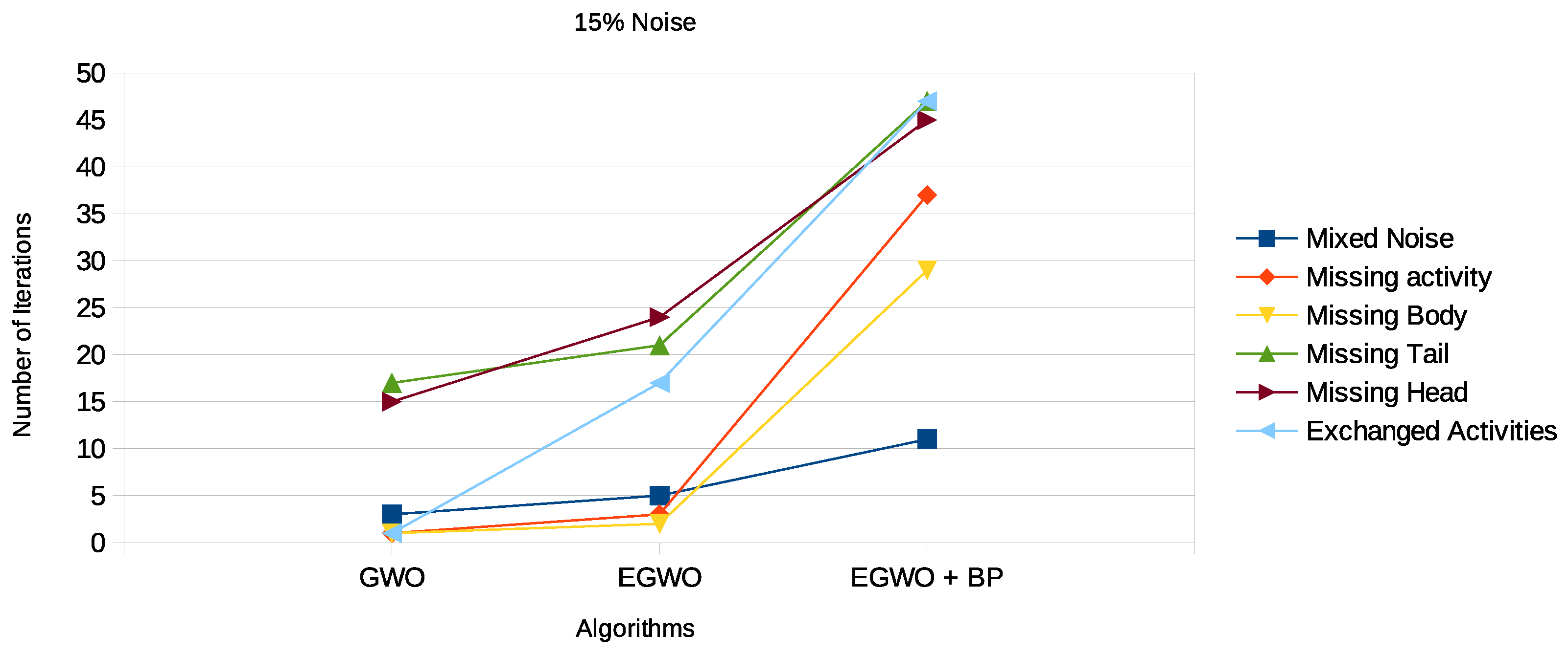
“Noise” in the log is defined as infrequent and improper behavior. Some activities in an event trace in a log may be missing a tail, head, or body; be exchanged with other activities; or be missing entirely. There may also be a mixture of all the noise types. In any case, noise might be a problem that prevents a process model from being discovered accurately. As it is similar to other low-frequency appropriate behavior in the log, noisy behavior is tough to spot. However, our approach to parsing activities makes noise easily detectable by the various algorithms. With the introduction of noise into the logs, the results for the mixed noise type in

Table 6. Addition of 5% noise to an event log.

	MN	MA	MB	MT	MH	EA
GWO	5.6	8	3.5	24	23	5
EGWO	10	15	6	34	36	32
EGWO + BP	14	39	32	48	48	49

MN = mixed noise, MA = missing activity, MB = missing body, MT = missing tail, MH = missing head, EA = activity.

,

Table 7. Addition of 10% noise to an event log.

	MN	MA	MB	MT	MH	EA
GWO	5	7	3	22	19	3
EGWO	8	13	4	29	31	27
EGWO + BP	12	38	31	48	46	47

MN = mixed noise, MA = missing activity, MB = missing body, MT = missing tail, MH = missing head, EA = activity.

and

Table 8. Addition of 15% noise to an event log.

	MN	MA	MB	MT	MH	EA
GWO	3	1	1	17	15	1
EGWO	5	3	2	21	24	17
EGWO + BP	11	37	29	47	45	47

MN = mixed noise, MA = missing activity, MB = missing body, MT = missing tail, MH = missing head, EA = activity.

and Figure 13, Figure 14 and Figure 15, respectively, show that the proposed algorithm indeed works for noisy logs as well.

Again, we see that the smaller the net, the more frequently the GWO algorithm finds the correct process model. The higher the noise percentage, the lower the probability the GWO algorithm will end up with the original process model. However, the EGWO is more robust to noise than just the GWO as the percentage of noise increases. The best of them all is the combination of the enhanced GWO with backpropagation (EGWO + BP); it has the highest noise tolerance level. The use of backpropagation helps the algorithm achieve better process models by comparing the desired output model to the achieved model outputs. The models are tuned by adjusting weights to narrow the difference between the two as much as possible. It also updates the weights backward, from output to input. It does not have any parameters to tune except for the number of inputs, as seen in Figure 13, Figure 14 and Figure 15. We can make the following observations by looking at the results for the different noise types. The enhanced gray wolf with backpropagation (EGWO + BP) algorithm for process mining can handle the exchanged activities noise type well. It has less impact on the algorithm’s performance than the missing body and missing activity noise types due to the random generation of the initial population. Additionally, it can handle the missing tail noise type better than the other two.

The missing head noise is the most significant, since process models cannot be completed successfully without the head. When tested on this particular noise, the GWO and its improved variant again underperformed. However, when EGWO was combined with backpropagation, the performance increased significantly. The algorithm’s capacity to both globally and locally search accounts for this behavior. We also evaluated our proposed method on real-life event logs; see the following section.

6.1. Evaluation

To conduct our evaluation, we selected Road Traffic Fine Management (RTFM) [41] real-life event logs publicly available in the 4TU.ResearchData repository. It has 11 activities and describes all the control-flow processes exhibited by any complete event log. A workflow log usually records the actual implementation process of the workflow model, and the log is usually made up of the workflow instance names “Case_id”, “Activity_name”, “Resource”, and “Timestamp”, etc. Among these, “Case_id” is used to identify the execution times of one workflow, such as case l or case 2; “Activity_name” is used to identify a specific activity of the workflow process, such as a1 or a2; “Resource” and “Timestamp” are used to represent the specific actors and execution time of the activity. We focus on the activity names. Due to the input errors that might occur, there may be missing records, duplicate records, and other reasons which may cause the workflow logs to be incomplete. For incomplete logs, we filtered them by removing an instance if its end event does not belong to the set of traces and if a task only has the end event without a corresponding start event or the start event without a corresponding end event for our analysis.

The activity names used in describing the various processes are as follows: (A) create fine; (B) receive result from prefecture; (C) insert date appeal to prefecture (D) send appeal to prefecture; (E) notify result appeal to offender; (F) appeal to judge; (G) send fine; (H) insert fine notification; (I) add penalty; (J) payment; (K) send for credit collection. In the above description, the uppercase letters A–K represent each activity name. According to the description, the flow control of activities in the event log [41] is depicted in the Petri net shown in Figure 16 using the traditional direct flows approach.

Our work used the semantics of the textual attributes to construct a process model reflecting direct follows, loops, and concurrency in a Petri net. All events have an event label (concept: name) specified using attributes from the XES standard [42]. We used the following steps to compute the semantic relatedness between these attribute names. Step 1. An event log L consists of several traces T; in each trace, several activities are arranged in an orderly manner via its timestamp attribute. We identify the activity names of each trace. Given an activity name in a trace, we tokenize each activity name which splits the textual attribute value into lowercase tokens based on white space and omit any numeric ones or stop words. For example, using Buijs and Joos’ [43] real-life event log, given s1 = “Confirmation of receipt”, s2 = “T02 Check confirmation of receipt”, s3 = “T04 Determine confirmation of receipt”, s4 = “T05 Print and send confirmation of receipt”, s5 = “T06 Determine necessity of stop advice”, and s6 = “T10 Determine necessity to stop indication”, we obtain: tokenize (s1) = [Confirmation, of, receipt], tokenize (s2) = [Check, Confirmation, of, receipt ] and tokenize (s3) = [Determine, Confirmation, of, receipt], s4 = [Print, and, send, Confirmation, of, receipt], s5 = [Determine, necessity, of, stop, advice], and s6 = [Determine, necessity, to, stop, indication].

Finally, the start and end activities are extracted from the list of activity names. The start activity is used as the hypernym with the assumption that, for each trace, the ordering of the activities from its first activity to the last activity are in a hypernym and hyponymy relations. This enables us to calculate their similarity based on their word sense. For instance, case 1 in BPIC [41] has the following activities: <CREATE FINE, RECEIVE RESULT APPEAL FROM PREFECTURE, SEND FINE, INSERT FINE NOTIFICATION, ADD PENALTY, PAYMENT, SEND FOR CREDIT COLLECTION∼$\langle A,B,G,H,I,J,K\rangle$.

Using Algorithm 1 to extract the start and end activities, CREATE FINE (start activity) and SEND FOR CREDIT COLLECTION (end activity), the remaining activities are assumed to be in a hypernym and hyponymy relation with the start activity. This assumption is made based on the fact that every event log describes a particular event type in an enterprise system. For instance, de Leoni et al. [41] described a real-life event log for an information system managing road traffic fines. Thus, we assume that process names used in such systems describe textual events related to road traffic and fines. Additionally, the event log WABO [43] contains records of the execution of the receiving phase of the building permit application process in an anonymous municipality. All textual descriptions of the process are expected to be related to receiving some form of a receipt.

Step 2 After identifying the start and end activities, we construct the subsume tree described in Section 4.1. The subsume tree is created based on ordering the activities from the root node. For example, take CREATE FINE. The activity following it is the next activity on the subsume tree. After constructing the tree, the information content of each activity name is calculated and based on the information content of their least common subsume value. A fuzzy causal matrix is generated. This is achieved by calculating the semantics of each phrase making up the name of an activity. For instance, we tokenize each activity name, remove all stop words, and create a set containing keywords of both activity names under comparison. These keywords are converted to vectors, and their similarity is calculated based on their semantics.

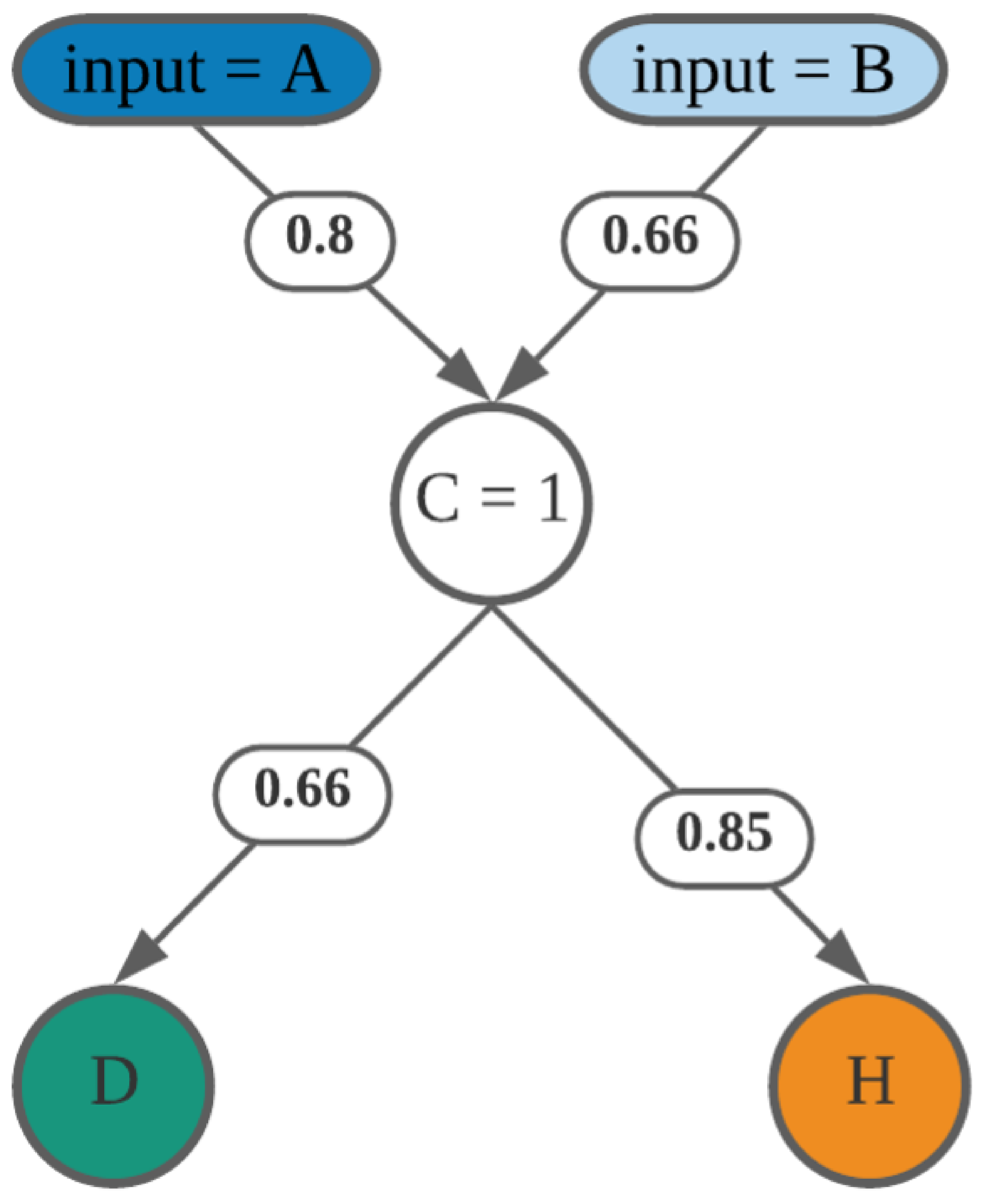
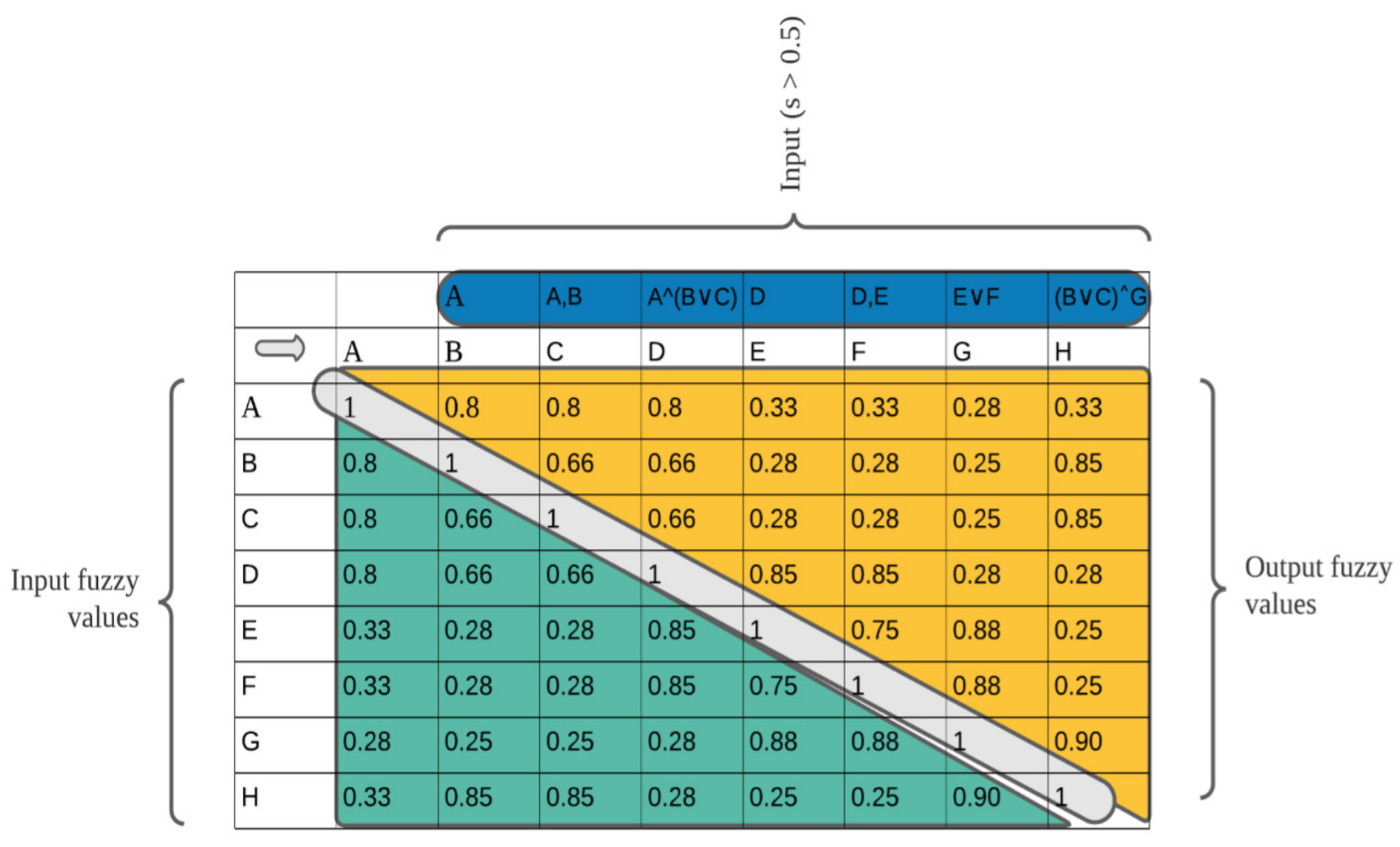
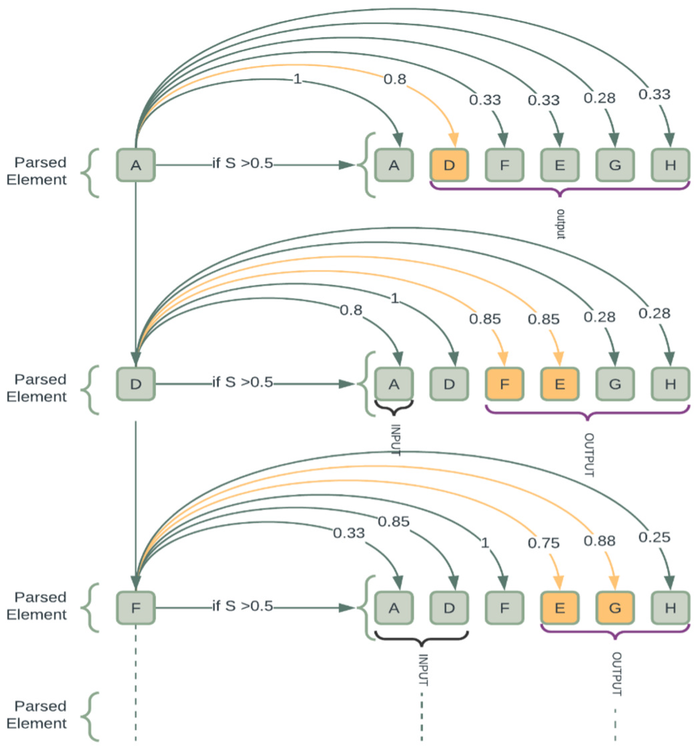
Each activity’s pair similarity values are calculated. Those activities with higher semantic value are considered to have a relation, as indicated in Table 2. For activity A in Table 2, activities $\langle B,C,G,H\rangle$ have higher values of relatedness than 0.5, and as such, share a relation with A. Activities with the same semantic value are in a choice relation with activities A, B, and C, and have the same similarity value with A. If two activities have different similarity values greater than 0.5 with another activity, those activities can be executed concurrently (see activities F and G in

Table 9. Fuzzy causal matrix generated from bpic[rtfm] using our approach.

$\overrightarrow{\mathbf{yields}}$	A	B	C	D	E	F	G	H	I	J	K
A	1	0.88	0.88	0.33	0.33	0.33	0.88	0.88	0.28	0.25	0.23
B	0.88	1	0.33	0.28	0.88	0.33	0.28	0.25	0.23	0.20	0.18
C	0.88	0.33	1	0.88	0.33	0.33	0.28	0.25	0.23	0.20	0.18
D	0.33	0.28	0.88	1	0.28	0.25	0.23	0.20	0.18	0.15	0.12
E	0.33	0.88	0.33	0.28	1	0.88	0.66	0.33	0.28	0.25	0.23
F	0.28	0.33	0.33	0.88	0.88	1	0.88	0.66	0.33	0.28	0.23
G	0.28	0.33	0.33	0.48	0.48	0.88	1	0.88	0.33	0.28	0.25
H	0.23	0.25	0.28	0.33	0.33	0.36	0.88	1	0.88	0.48	0.33
I	0.18	0.20	0.23	0.25	0.28	0.33	0.25	0.88	1	0.88	0.33
J	0.15	0.18	0.20	0.23	0.25	0.28	0.33	0.36	0.88	1	0.90
K	0.12	0.15	0.18	0.20	0.23	0.25	0.28	0.33	0.36	0.88	1

). If there is only one activity with semantic value greater than 0.5, those activities are in a sequential relation (see activities I and J in Table 9).

The log has 1424 instances. As for space, we selected 37 from it, as seen in

Table 10. Event-log workflow of BPIC [41] generated by our method.

Case_ID	Activity_Name	Atomic Representation
Case 1	Create fine	A
Case 2	Create fine	A
Case 3	Create fine	A
Case 1	Receive result appeal from prefecture	B
Case 4	Create fine	A
Case 3	Insert date appeal to prefecture	C
Case 1	Notify result appeal to prefecture	E
Case 2	Receive result appeal from prefecture	B
Case 3	Send appeal to prefecture	D
Case 1	Appeal to judge	F
Case 5	Create fine	A
Case 4	Send fine	G
Case 3	Appeal to judge	F
Case 5	Insert fine notification	H
Case 2	Notify result appeal to prefecture	E
Case 3	Send fine	G
Case 2	Send fine	G
Case 2	Insert fine notification	H
Case 3	Insert fine notification	H
Case 5	Add penalty	I
Case 3	Add penalty	I
Case 4	Insert fine notification	H
Case 3	Payment	J
Case 4	Add penalty	I
Case 1	Send fine	G
Case 1	Insert fine notification	H
Case 5	Payment	J
Case 1	Add penalty	I
Case 1	Payment	J
Case 2	Add penalty	I
Case 1	Send for credit collection	K
Case 3	Send for credit collection	K
Case 2	Payment	J
Case 2	Send for credit collection	K
Case 4	Payment	J
Case 4	Send for credit collection	K
Case 5	Send for credit collection	K

and then reconstructed the workflow net in terms of Petri based on our methodology. The event log has 11 activities. Note that the activities’ names are being represented as $\langle A,B,C,D,E,F,G,H,I,J,K\rangle$. Table 10 illustrates the workflow log generated by our method by selecting a similarity threshold of 0.5 to get more information content but also to eliminate rare event occurrences. According to the semantic relationship matrix generated, the reconstructed process model of the event log is shown in Figure 17.

After creating the process model using the methodology we suggested, we discovered that activities A and G were not carried out in a synchronous relationship in the predefined process model in Figure 16. A was in a sequence relationship with H and I. Further research into the business process revealed that, in reality, there is a clear causal relationship between activities A and G. The two tasks being carried out in sync did alter the outcomes of the tasks done and could increase the effectiveness of the process execution. Therefore, in this regard, the method of event activity parsing we have suggested for use in process mining satisfies the requirements for a process discovery algorithm’s actual implementation. We have compared our proposed method with existing state-of-the-art algorithms in Section 6.1.

6.2. Comparative Analysis

Process discovery aims to understand how the events reported in the event log have transpired. Process discovery becomes an intrinsically descriptive process. It is, therefore, reasonable to compare the learned process models on the same sequence from which the process models are learned to assess the correctness of the found process model. Several authors have used the training-log-based assessment technique [17,44] in the literature for comparison techniques. We employed such a metric to draw comparisons with other process discovery methods. As indicated in

Table 11. Event logs.

Model	Events	States	PI	${\mathit{B}}_{\mathit{R}}$	${\mathit{B}}_{\mathit{P}}$	Par	Loops	nfc	conc	dup
1	4	3	150	1	1	0	1	0	0	0
betaSimplified	13	4	150	1	1	0	-	1	1	2
a12	19	92	150	1	0.992	-	2	-	-	-
a5	7	13	150	1	1	1	1	-	-	-
herbstFig6p33	8	8	150	1	1	-	-	-	-	1
1Skip	4	6	150	1	0.732	0	1	0	1	1
bn1	41	40	150	1	1	-	-	-	-	-
bn2	41	40	150	1	1	-	1	-	-	-
bn3	42	150	150	1	0.999	-	1	-	-	1
choice	10	7	150	1	1	-	-	-	-	-
DriversLicense	7	8	150	1	1	-	-	1	-	-
driversLicense1	11	87	150	1	1	1	1	1	1	1
flightCar	6	8	150	1	1	-	-	-	1	1
herbstFig3p4	12	32	150	1	0.999	-	1	-	1	-
herbstFig5p19	8	6	150	1	1	1	-	-	1	1
herbstFig5p1AND	3	4	150	1	1	-	-	-	-	1
herbstFig6p36	12	2	150	1	1	-	-	1	-	-
herbstFig6p37	14	51	150	1	1	-	-	-	1	-
herbstFig6p38	7	5	150	1	1	3	-	-	-	-
herbstFig6p39	5	11	150	1	1	1	-	-	1	1
herbstFig6p41	16	12	150	1	1	-	-	-	1	-
2Optional	4	4	150	1	1	-	1	-	-	-
parallel5	10	110	150	1	1	-	-	-	1	-
repair2	8	48	150	1	1	-	1	-	-	-

PI = process instance, B_R = behavioral recall, B_P = behavioral precision, Par = parallelism, nfc = non-free choice, conc = concurrency and dup = duplicates.

, we employed 24 benchmark process models and introduced noise using the ProM6.1 framework’s AddNoiseFilter plugin.

Six forms of artificial noise have been published in the literature [17,45], as detailed in Section 6 when comparing the performances of the algorithms employed in our suggested technique.

Our suggested solution was not implemented in the ProM framework; we developed it in Python using the Pm4Py package as a comparison. For the sake of brevity, we mixed all possible noise types in our tests. We implemented 10% and 5% noise levels. To make a fair comparison, we used Equations (34)–(42) to compute each log’s behavioral accuracy and recall and compared our results to those reported in the literature.

Results from the 24 related event logs that correlate with the found process models are summarized in Table 11. Unlike the formal techniques of ${\alpha }^{+}$ and ${\alpha }^{++}$ and the genetic miner, known to overfit the noise in event logs, heuristics miners are immune to noise. Multiple trials revealed that the ${\alpha }^{++}$ implementation always failed to yield results. As for these missing values, all the metrics were given a score of 0.00. In addition, the genetic mining method creates 11 instances of erroneous outputs due to the state space analysis needed to calculate the behavioral appropriateness metric.

As can be seen in

Table 12. Performance comparison of our method to existing algorithms based on robustness to noise in an event log.

NPL (%)	Algorithm	PM	F	${\mathit{A}}_{\mathit{b}\mathit{a}}$	Acc	${\mathit{B}}_{\mathit{R}}$	${\mathit{B}}_{\mathit{P}}$	$\mathit{A}\mathit{c}{\mathit{c}}_{{\mathit{B}}_{\mathit{R}},{\mathit{B}}_{\mathit{P}}}$
	${\alpha }^{+}$	0.11	0.83	0.85	0.84	0.87	0.62	0.74
	${\alpha }^{++}$	0.00	0.79	0.65	0.72	0.75	0.63	0.69
5 all mixed noise	Heuristics	0.88	0.98	0.87	0.93	0.98	0.94	0.96
	Genetics	0.74	0.99	0.63	0.81	0.98	0.91	0.95
	Proposed Method	0.90	0.99	0.88	0.94	0.98	0.93	0.96
	${\alpha }^{+}$	0.08	0.80	0.84	0.82	0.84	0.59	0.72
	${\alpha }^{++}$	0.00	0.73	0.80	0.76	0.64	0.64	0.64
10 all mixed noise	Heuristics	0.88	0.99	0.86	0.92	0.99	0.95	0.97
	Genetics	0.51	0.97	0.59	0.78	0.94	0.78	0.86
	Proposed Method	0.89	0.98	0.87	0.93	0.98	0.96	0.97

NPL = noise percentage level, F = fitness, A_ba = advanced behavioral appropriateness, Acc = accuracy, B_R = behavioral recall, B_P = behavioral precision, A_ccBR,BP = accuracy of B_R and B_P.

, the algorithm with the highest average score across all noise levels for the parsing measure (PM), fitness (f), advanced behavioral appropriateness ($A_{ba}$), accuracy (Acc), behavioral recall ($B_R$), behavioral precision ($B_P$), and accuracy of behavioral recall and precision metrics ($Ac{c}_{BR,BP}$) is bold faced. It is shown that our suggested technique produces accurate results that are resilient and not substantially different from the results produced by heuristics miners for all noise levels. Our suggested approach can detect more sophisticated process structures, such as duplicate and invisible activities, since it does not see events in the log as syntactic labels. Instead, it uses the semantics underlying those labels to develop a process model.

Our approach’s resistance to noise stems from the fact that we use semantics to disentangle event activities. If a train ticketing system keeps an event log, for instance, all of its procedures should include relevant information in the context of railway ticketing; otherwise, an activity with the information content of a supermarket might be regarded as noise. To compare our proposed model comprehensively in the future with the current approaches, we intend to develop it as a ProM plugin to compute the fitness of mined process models through compliance testing. Despite this, our suggested method has shown more potential in dealing with noise, which is inescapable in any event log.

7. Conclusions

Everyday transactions are made on several enterprise systems. These transactional changes leave traces, which are recorded as event logs from which insights into these systems’ operations and execution can be realized. Unfortunately, sometimes, these transactions deviate from the predefined organizational workflow structure due to noise. Therefore, management and process mining practitioners may want to reconstruct this workflow according to the actual situation to mitigate all shortcomings, and if there are any, to seek redress. To overcome the limitation of the existing process mining algorithms, this paper presented a new approach to parsing activities in an event log for process mining using the information content of the least common subsume of event log attributes. This approach was subsequently used in designing an enhanced gray wolf optimizer with backpropagation to mine process models.

After introducing process mining and its practical relevance, we described the parsing process of activities and presented the gray wolf and backpropagation algorithms. Using an enhanced gray wolf optimizer with backpropagation for an event log containing noise provides a promising perspective for process mining. After introducing a new framework for representing processes (the fuzzy causal matrix), we went into the specifics of three algorithms: the gray wolf optimizer, the Levy flight, and backpropagation. These algorithms’ fitness metrics depend on successfully parsing the activities in the event log. However, fitness parsing semantics are stopped when the gray wolf optimizer becomes trapped in the local optimum. Then, for improved results, Levy flight is included to redistribute the individuals stochastically in the search space. However, modifying the GWO with the Levy flight did not offer so much; hence, we introduced a backpropagation algorithm to guide the search to the local space due to its strong local search ability to give a good fitness measure. In the experimental section, we provided the enhanced grey wolf optimizer with backpropagation algorithm for process mining from event logs with and without noise. The performance variations among the gray wolf optimizer (GWO), the enhanced gray wolf optimizer with levy flight (EGWO), and the enhanced gray wolf optimizer with backpropagation (EGWO + BP) were the subjects of our study.

The key finding is that the performance of EGWO + BP, with the best fitness measure, appears to be superior for both noise-free and noisy event logs. We examined the performance behavior of the EGWO + BP for various noise types, including missing head, a missing body, missing tail, missing activity, exchanged activities, and mixed noise. We found that the missing-body and missing-activity noise types present unique mining challenges because they frequently introduce unnecessary connections into the process model. Though the EGWO + BP has shown high tolerance to missing body and missing activity noise types, it could still be enhanced to improve the noise tolerance level, especially for those two noisy types. Furthermore, the workflow instances may diverge from those in the preset models due to the company’s changing internal and external environments; therefore, modelers must reconstruct the model per the actual scenario. This article developed a new method of parsing event activities by using the information content of their least common subsume values to automatically deduce the actual structure of the relationship between activities and thus implement workflow reconstruction. An actual simulated case study demonstrated the method’s viability and applicability. To strengthen and extend the method’s mining capability, follow-up studies will concentrate on how to automatically derive sub-processes and mine other attributes, such as the relationship between resources in an event log. The proposed algorithm mines process models that are robust to noisy logs and can be used by process modelers to gain insight into their systems. The next step of this project is to turn the suggested approach into a ProM6 plugin. This will give process miners more choices when doing process analysis.