Abstract
Inspired by real-world sheepdog herding behavior, in this paper, four behavior-based herding algorithms have been proposed for the social force model-based sheep herd. First, a basic behavior-based herding algorithm is designed where four types of critical sheep are rigorously defined. The decision of the sheepdog is made by constantly checking the positions of these four critical sheep. Then, on top of this basic herding algorithm, two extra mechanisms are considered to improve the performance of the basic herding algorithm, namely the dynamic far-end mechanism and the pausing mechanism, thus, forming the other three herding algorithms. The dynamic far-end mechanism helps to avoid the undesired circling behavior of the sheepdog around the destination area, while the pausing mechanism can greatly reduce the control cost of the sheepdog. To validate the effectiveness of the proposed herding algorithms, comprehensive tests have been conducted. The performance of the four algorithms is evaluated and compared from three aspects, namely, success rate, completion step, and control cost. Moreover, parameter analysis is provided to examine how different design parameters will affect the performance of the proposed algorithm. Finally, it is shown that when the size of the sheep herd increases, as expected, it takes more time and control effort to complete herding.
1. Introduction
Swarm movements for living creatures exist widely in nature, such as the V-shaped migration of migratory birds [1], the swarming phenomenon of bees [2], the coordination and self-organization of ant colonies, and the vortex swimming of sardine swarms [3], which have attracted extensive attention from researchers in various related fields. Fundamental works on swarm systems can be found in Aoki [4], Reynolds [5], and Huth and Wissel [6,7], just to name a few, leading to fruitful subsequent results. Various collective and cooperative behaviors of swarm systems have found engineering applications in many scenarios, for instance, navigation of unmanned aerial vehicles flying in formation [8,9], group patrolling of unmanned vehicles [10,11], design and application of mobile sensor network in multi-environment [12], cooperation of swarm robots to complete collective tasks [13], and cooperative exploration by a flock of underwater vehicles [14,15].
Sheep herd is a typical swarm system, and the shepherds are good at teaching sheepdogs how to work, that is, to control a swarm system. While it was not until recently that people began to study the underlying mechanism of herding. In 1996, Schultz [16] used genetic algorithms to create decision rules to replicate sheep herding behavior. Later, John [17] used cognitive modeling to enable a T-rex to drive a flock of raptors from one territory to another. Vaughan [18] constructed a potential field model of cluster behavior and used it to study generalized cluster control. The side-to-side idea for herding was initiated by [19,20], where a global dynamic road map should be planned to provide milestones and steering points. Since then, a large number of studies on herding have emerged based on the side-to-side approach. Bennett [21] proposed circling behavior, where sheepdogs move on the rear periphery of the flock. Fujioka [22] proposed a V-formation control method. Behind the flock, three points are dynamically selected to form a V-formation, and the shepherd switches positions among these three points. Zhang [23] modeled the sheep by three characteristics: dispersal preference, predator avoidance, and aggregation preference, and proposed the so-called outmost push strategy. It turns out that this strategy also leads to side-to-side motion. In practice, the herding algorithms can be used to drive passive or non-cooperative swarm robots from one location to another [24,25,26,27]. Song [24] formalized the concept of a cage in a topological way to guide a group of mobile agents to a specified goal region. The ideas of [25,26,27] were similar, that is, to let multiple dogs encircle the flock, and in this way, herding can be achieved by letting the dogs move towards the destination in formation.
In this paper, inspired by real-world sheepdog herding behavior, four behavior-based herding algorithms are proposed for the social force model-based sheep herd. The research flowchart of this paper is shown in Figure 1.
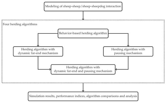
Figure 1.
Research flowchart.
Sheep Herd Modeling: In this paper, we use the social force model [28,29,30,31,32] to describe the behavior of the sheep herd, where the interaction between individuals is treated as force, and the resultant force of all the neighbors forms the social force. In particular, in this paper, the force is fully determined by the relative position of two individuals, forming four zones from inside to outside. The first, inner-most zone is the repulsive zone; the second zone is a neutral zone where no force is activated; the third zone is the attractive zone; the fourth, outer-most zone is the zone where the two individuals are beyond the perceptive range of each other, and, thus, again no force is activated.
Behavior-based Herding Algorithm: The basic idea of the herding algorithm, like in [19,20], is to let the sheepdog move behind the sheep herd in a side-to-side manner, forming a repeated semi-circle route. Based on this idea, a basic behavior-based herding algorithm is first designed, where four types of critical sheep are rigorously defined. The decision of the sheepdog is made by constantly checking the positions of these four critical sheep. (The initial version of this part of the work was documented in our previous work [33].) While different from the existing results, we do not set external steering points or milestones outside the sheep herd to achieve side-to-side motion, but use critical sheep as temporary reference points. By doing so, the sheepdog shall stick to the contour of the sheep herd, which would greatly reduce the odds of sheep herd fragmentation due to improper route of the sheepdog as mentioned in [19,20]. Moreover, on top of this basic herding algorithm, two extra mechanisms are considered to improve the performance of the basic herding algorithm, namely the dynamic far-end mechanism and the pausing mechanism, thus, forming the other three herding algorithms.
Related Works and Contributions: In contrast to the existing works, the contributions of this work are summarized as follows. (i) In [21], the direction of the dog’s circling is switched based on the centroid of the flock. However, when the number of sheep is large, the centroid of the flock might not be available. Instead, in our work, we put a limit on the perceptive range of the sheepdog. Moreover, the sheep might be vision-blocked by other sheep from the viewpoint of the sheepdog, even if it is within the perceptive range of the sheepdog. At each step, the sheepdog can only decide based on the visible sheep to it, which makes the algorithm of this work more practical. (ii) Some existing works, say, [23], assume that the boundary of the destination area is soft. In this way, once a sheep is driven into the destination area, it cannot go outside by itself. While, in this paper, we consider the more challenging scenario where no specific requirement is imposed on the destination area, which makes herding more difficult in the final stage when the sheep herd is around the destination area. To tackle this problem, we have designed a dynamic far-end mechanism that can effectively solve the circling issue in the final stage of herding. (iii) In the real world, the sheepdog sometimes pauses when herding. This is because the “inertia” of a big sheep herd is large, and, thus, it takes time for the repulsive force imposed by the sheepdog to propagate over the sheep herd. The appropriate pause may save energy for the sheepdog, thus making herding more cost-effective. Therefore, we have further proposed a pausing mechanism, which can greatly reduce the control cost, as validated by the simulation results.
2. Notation
Let and denote the sets of real numbers and positive integers, respectively. Given , . Given a set with a finite number of elements, let denotes the cardinality of the set . For a vector , denote the Euclidean norm of x. Given a point and a region , the distance between x and is defined by
Given angle , the planar rotation matrix is defined by
For a nonzero vector , let
denote the unit directional vector of x. Moreover, the left-hand side area of x is defined by
and the right-hand side area of x is defined by
For two nonzero vectors , the angle between x and y is given by
where denotes the inner product of the two vectors . For , define the following saturation function
where denotes the saturation threshold. Suppose there are three distinct points . For point x, if
then point x is called vision-blocked by point z for point y. Obviously, vision-block is mutual, i.e., if point x is vision-blocked by point z for point y, then it follows that point y is vision-blocked by point z for point x.
3. System and Task Description
In this paper, as illustrated in Figure 2, we consider the herding problem, i.e., to drive a sheep herd from an initial location to some predetermined destination area by a single sheepdog. Throughout this paper, it is assumed that the positions of all the sheep and the sheepdog are expressed in a common coordinate.
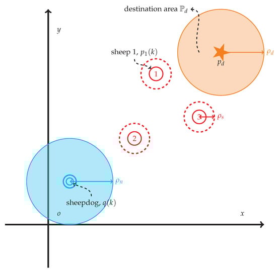
Figure 2.
An example of the herding problem with 3 sheep, denoted by red circles with labels, and 1 sheepdog, denoted by a blue circle. The destination area (in orange) is centered at .
Suppose the sheep herd consists of N sheep. For , the motion of the ith sheep is governed by the following equation:
where T denotes the sampling period, denote the position and velocity of the ith sheep at the kth step, respectively.
The motion of the sheepdog is governed by the following equation:
where denote the position and velocity of the sheepdog at the kth step, respectively.
For , , define
At step k, for sheep i, if sheep j is not vision-blocked by any other sheep or the sheepdog, and satisfies where denotes the perceptive radius of the sheep, then sheep j is called visible to sheep i. Let denote the label set of all the sheep visible to sheep i at step k.
Similarly, at step k, for sheep i, if the sheepdog is not vision-blocked by any other sheep, and satisfies , then the sheepdog is called visible to sheep i. Define if the sheepdog is visible to sheep i at step k, and otherwise.
At step k, for the sheepdog, if sheep i is not vision-blocked by any other sheep, and satisfies where denotes the perceptive radius of the sheepdog, then sheep i is called visible to the sheepdog. Let denote the label set of all the sheep visible to the sheepdog at step k.
If , then the center of the visible sheep for the sheepdog at step k is defined by
The above definitions are illustrated by an example shown by Figure 3, where sheep 2 is vision-blocked by sheep 5 for the sheepdog. In this scenario, , , and .
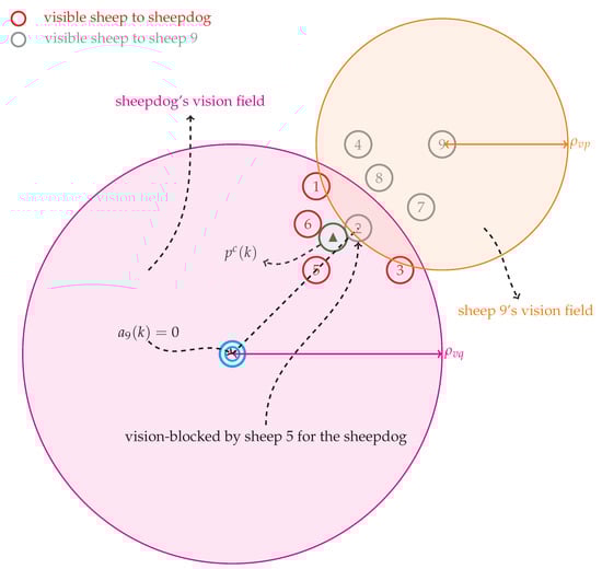
Figure 3.
An example of the visual fields of sheep and sheepdogs.
In this paper, we assume that the motion of the sheep herd follows the social force rules. To be more specific, for , the velocity of the ith sheep is set as follows:
where denotes the upper limit for the speed of sheep. denotes noise, which takes the following form
where uniformly take random values from interval . represents the force imposed by the sheepdog, which is given by
where
with denoting the intensity of sheepdog-to-sheep repulsive force, denoting the allowable minimal distance between sheep and sheepdog. The plot of is shown by Figure 4a with , , and . represents the force imposed by other sheep, which is given by
where
with denoting the intensity of sheep-to-sheep repulsive and attractive force, respectively. denotes the minimal sheep-to-sheep safety distance. The plot of is shown by Figure 4b with , , , , and . For (9) to make sense, it must hold that . By (8), the sheep herd tends to get together when they are scattered yet not overly sparse, and, in the meantime, keep minimal inter-sheep distance. Note that in between attractive and repulsive areas, there exists some certain area, dictated by and , within which there is no force between two sheep. In this way, the sheep herd can reach and maintain a static balance.
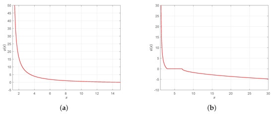
Figure 4.
Plots of functions and . (a) Plot of with , , . (b) Plot of with , , , , .
The sheep herd polygon is defined by
Given , the destination area for the sheep herd is defined by
for some . should be chosen such that the following two requirements can be simultaneously satisfied:
and
Mathematically, the herding problem considered in this paper is to design for the sheepdog, under the initial condition
and
such that, for all , and all ,
and
for some , where K is the step limit.
4. Herding Algorithm
By the observation of the behaviors of the real-world sheepdog, in this section, four behavior-based herding algorithms will be proposed in order. First, a basic behavior-based herding algorithm is designed where four types of critical sheep are rigorously defined. The decision of the sheepdog is made by constantly checking the positions of these four critical sheep. Then, on top of this basic herding algorithm, two extra mechanisms are considered to improve the performance of the basic herding algorithm, namely the dynamic far-end mechanism and the pausing mechanism, thus, forming the other three herding algorithms.
4.1. Behavior-Based Herding Algorithm
To begin with, we introduce four important directions:
denotes the unit vector from the center of the visible sheep to the destination. and are the left and right perpendicular vector of , respectively. denotes the unit vector from the sheepdog to the center of the visible sheep. Based on , we further define
Based on the direction of , () is the label set of the sheep which are on the left (right) hand side of the sheepdog.
Next, we define four types of critical sheep. To this end, define four functions as follows
where and . For the ith sheep, , and denote the projections of to the directions of , and , respectively. Then, define
and
where and are called left and right anchor sheep, respectively. For the sheep on the left (right) hand side of the sheepdog along the direction of , the sheep with the least projection of to the direction of constitute the set of (), within which the nearest sheep to the sheepdog is defined to be the left (right) anchor sheep. Moreover, define
and
where and are called left and right front sheep, respectively. The sheep with the maximal projection of to the direction of () constitute the set of (), within which the farthest sheep to the sheepdog is defined to be the left (right) front sheep.
Finally, define the left and right turning angles by
Examples illustrating the aforementioned definitions are shown in Figure 5 and Figure 6. Now, the behavior-based herding algorithm is given by Algorithm 1.
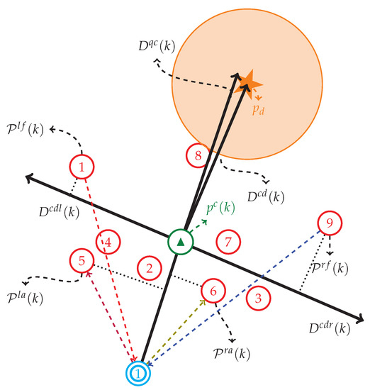
Figure 5.
An example illustrating the definitions of , , , , , , , and .
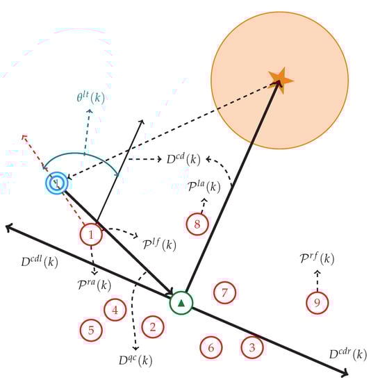
Figure 6.
An example illustrating the definitions of , , , , , , , , and .
Below we make some explanations for Algorithm 1. To begin with, we check the algorithm termination condition, i.e., the step limit is hit, or the herding task is fulfilled. If neither of these conditions is satisfied, the algorithm continues, calculating the next move for the sheepdog. The basic idea of the herding algorithm, like in [19,20], is to let the sheepdog move behind the sheep herd in a side-to-side manner, forming a repeated semi-circle route. While different from the existing results, we do not set external steering points or milestones outside the sheep herd to achieve side-to-side motion, but use critical sheep as temporary reference points. By doing so, the sheepdog shall stick to the contour of the sheep herd, which would greatly reduce the odds of sheep herd fragmentation due to improper route of the sheepdog as mentioned in [19,20]. In general, there are two main issues to address. First, how to make the sheepdog stick to the contour of the sheep herd? We solve this issue by defining anchor sheep, which are dynamically changing as the sheepdog moves. When the sheepdog uses these anchor sheep as reference points, the detouring angle makes the route bend in the direction of outliers, thus preventing the sheepdog from breaking into the sheep herd directly. Second, how to determine the turning point for the sheepdog? The turning behavior is activated when two criteria are met simultaneously. On the one hand, the entire sheep herd is on one side of the line connecting the sheepdog and the far end of the destination, which is chosen to be the destination center in Algorithm 1. On the other hand, the turning angle should be small enough, less than the turning-angle threshold . In Algorithm 1, the state-flag is used to identify the moving direction of the sheepdog at step k.
| Algorithm 1 Behavior-based Herding Algorithm |
|
4.2. Herding Algorithm with Dynamic Far-End Mechanism
Some existing works, say, [23], assume that the boundary of the destination area is soft. In this way, once a sheep is driven into the destination area, it cannot go outside by itself. While, in this paper, we consider the more challenging scenario where no specific requirement is imposed on the destination area, which makes herding more difficult in the final stage when the sheep herd is around the destination area. To tackle this problem, we improve Algorithm 1 by adding the dynamic far-end mechanism, which is detailed as follows. Define the dynamic far-end as
The definition of is illustrated by Figure 7. By , we use the line connecting the sheepdog and the dynamic far end rather than the static destination center as in Algorithm 1 to determine whether all the sheep are on one side of the line or not, which is one of the criteria to determine the turning point for the sheepdog. In this way, we can avoid the failure that probably happens when the sheep herd is around the destination. With the dynamic far-end mechanism, the herding algorithm is given by Algorithm 2.
| Algorithm 2 Herding Algorithm With Dynamic Far-end Mechanism |
|
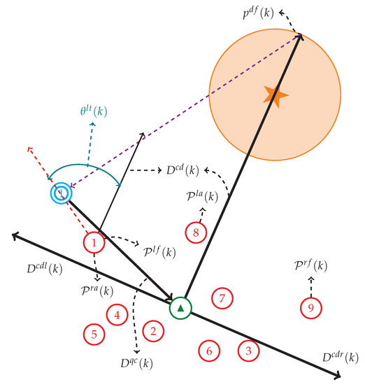
Figure 7.
An example illustrating the dynamic far–end mechanism.
4.3. Herding Algorithm with Pausing Mechanism
In the real world, the sheepdog sometimes pauses when herding. This is because the “inertia” of a big sheep herd is large, and thus it takes time for the repulsive force imposed by the sheepdog to propagate over the sheep herd. The appropriate pause may save energy for the sheepdog, thus making herding more cost-effective. Inspired by this observation, we propose a pausing mechanism as follows.
Define the back declination angle as
The definition of is illustrated by Figure 8. means the sheepdog is exactly behind the center of the visible sheep along the direction of . Around this spot, the repulsive force on the sheep herd nearly points to the destination center.
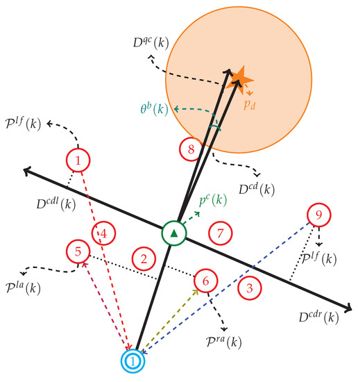
Figure 8.
An example illustrating the definition of .
Moreover, define the approaching ratio as
Let be the approaching threshold for . Whenever , the sheepdog will approach the sheep herd.
Based on and , the pausing mechanism is described as follows. Let be the back-declination-angle threshold. When , the sheepdog will decide whether to pause or not. Let be the pausing threshold for , satisfying . Under the condition that , if , the sheepdog will pause to drive the sheep herd towards the destination center. With the pausing mechanism, the herding algorithm is given by Algorithm 3.
| Algorithm 3 Herding Algorithm With Pausing Mechanism |
|
4.4. Herding Algorithm with Dynamic Far-End and Pausing Mechanism
Finally, by combining both the dynamic far-end and pausing mechanism with the herding algorithm, we obtain Algorithm 4.
| Algorithm 4 Herding Algorithm With Dynamic Far-end and Pausing Mechanism |
|
5. Test and Analysis
In this section, we will test and analyze Algorithms 1–4. First, we will show the typical herding process under Algorithms 1–4. Next, we will evaluate and compare the performance of Algorithms 1–4 from three aspects, namely, success rate, completion step, and control cost. Finally, we will perform parameter analysis to see how different parameters will affect the performance of the proposed algorithm.
5.1. Typical Herding Process under Algorithms 1–4
First of all, it will be shown that with proper parameter selection, all Algorithms 1–4 can achieve successful herding. The simulation conditions are detailed as follows.
- destination area related parameters: , .
- sheep herd related parameters: , , , , , , , , , .
- sheepdog related parameters: , .
- algorithm design parameters and thresholds: , , , , , .
- The initial positions for the sheep are given by , , , ,, , , , , , , , , , , , , , , , , , , .
- The initial position for the sheepdog is given by .
Note that the values of algorithm design parameters and thresholds are determined by trial and error through comprehensive numerical simulation data, where more detailed analyses are given in Section 5.4. Figure 9 shows that the herding task has been successfully achieved under all Algorithms 1–4.
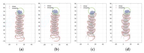
Figure 9.
Motion trajectories of the sheep herd and sheepdog under Algorithms 1–4. (a) Algorithm 1. (b) Algorithm 2. (c) Algorithm 3. (d) Algorithm 4.
5.2. Evaluation and Comparison of Algorithms 1–4
Now, we will evaluate and compare the performance of Algorithms 1–4 from three aspects, namely, success rate, completion step, and control cost, which are defined as follows.
- success ratewhere, for a given algorithm, we conduct many tests subject to different initial positions for the sheep and sheepdog, out of which many tests are successful. In this subsection, is set to be .
- Given an algorithm, consider the successful tests, labeled from 1 to . For the ith successful test, suppose the completion step is . Then, the completion step for the associated algorithm is defined to be
- Given an algorithm, consider the successful tests, labeled from 1 to . For the ith successful test, define the control cost asThen, the control cost for the associated algorithm is defined to be
In this section, we take the same simulation conditions as in Section 5.1. The initial positions for the sheep is with the range of . The data of simulation results are summarized by Table 1, which are also illustrated by Figure 10, Figure 11 and Figure 12.

Table 1.
The data of simulation results.
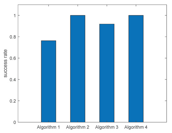
Figure 10.
The success rate of Algorithms 1–4.
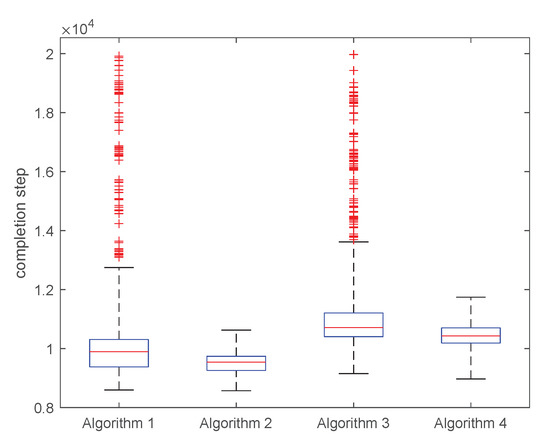
Figure 11.
The completion step of Algorithms 1–4.
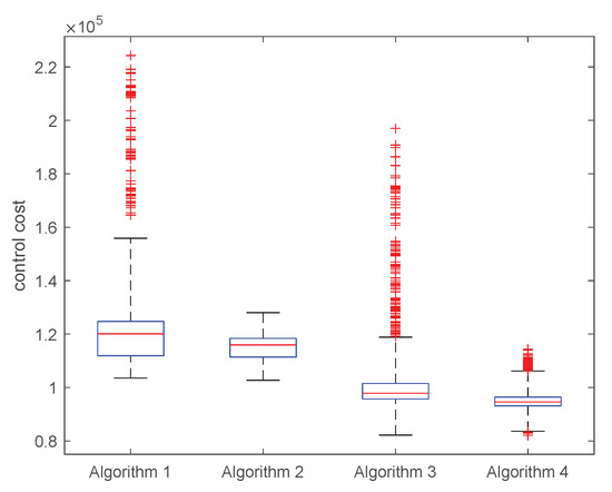
Figure 12.
The control cost of Algorithms 1–4.
In what follows, we will compare and explain the different performance of Algorithms 1–4. We begin with Algorithms 1 and 2. From Table 1, it can be seen that the success rate of Algorithm 2 is 100%, while the success rate of Algorithm 1 is much lower, around 76%. For most of the cases, the failure of Algorithm 1 happens at the final stage of herding, i.e., when the sheep herd are around the destination area. Note that one of the criteria for the sheepdog to change moving direction is that all the sheep are on one side of the line connecting the sheepdog and the far-end of the destination area, which is chosen to be the destination center in Algorithm 1. However, this criterion cannot be easily met when the destination area is not large enough since, in such case, the resulting line would probably pass through the sheep herd in the final stage, and, thus, the sheepdog keeps circling around the destination area without turning direction, thus leading to a failure. In contrast, in Algorithm 2, the far-end of the line has been changed from the destination center to the dynamic far-end, which is on the boundary of the destination area. This modification makes it easy for the turning criterion to be met, which helps to avoid the circling behavior of the sheepdog. Regarding the other two performance indices, i.e., completion step and control cost, as seen by Figure 11 and Figure 12, Algorithm 2 exhibits some little advantage in comparison with Algorithm 1. While, since there could still be occasional successful cases of Algorithm 1 where the sheepdog circling movement does happen in the final stage, the upper limits for the complete step and control cost of Algorithm 1 are much higher than those of Algorithm 2.
Next, we compare Algorithms 1 and 3. As illustrated before, since both Algorithms 1 and 3 adopt the destination center as the far end; they both suffer from the circling problem in the final stage. As a result, the success rates of both these two algorithms are below 100%. Algorithm 3 improves Algorithm 1 by introducing the pausing mechanism, which brings about two benefits. The major benefit is the control cost of Algorithm 3 is significantly reduced, up to almost 17% as shown by Table 1. The reason is obvious that the sheepdog would pause from time to time when the timing is appropriate. The minor benefit is in the final stage; the pausing mechanism helps eliminate the circling behavior, which in turn increases the success rate in comparison with Algorithm 1. Moreover, the simulation data, on the other hand, shows that the pausing mechanism increases the completion step on the magnitude of 7%. In all, there would be a compromise when both the completion step and the control cost are taken into consideration. As aforementioned, the circling problem will occur to Algorithms 1 and 3 only for small , which will disappear when the destination area becomes larger and larger. The specific data are shown by Figure 13 when increases from 8 to 11 under Algorithm 3.
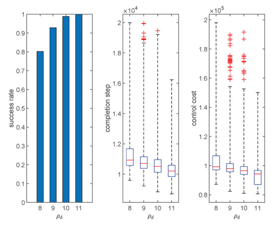
Figure 13.
The influence of the size of the destination area on Algorithm 3.
Finally, if we attach both the dynamic far-end and pausing mechanism to Algorithm 1, as expected, the success rate becomes 100% with the completion step increasing a little bit and the control cost is greatly reduced, as shown in Table 1.
5.3. Comparison with Other Existing Results
In this subsection, we will compare the performance of Algorithm 4 with that of the existing algorithm proposed by Bennett [21]. Bennett’s algorithm mimics the circling behavior of sheepdogs. Driving sheep herd is achieved by alternating the direction of circling. The motion vector is calculated according to the position of the leftmost or rightmost sheep from the perspective of the sheepdog, and then the direction of the sheepdog’s circling motion is obtained by adding an angle offset. The sheepdog should describe a circle of around 1/4 to 1/3 of the way around the sheep herd. The sheepdog’s alternating between two circling directions depends on the position of the sheep with respect to the goal and the angle of . Once a circling pattern is formed, the sheepdog will keep in this pattern until a termination condition is met. We compare the performance of Algorithm 4 with that of Bennett’s algorithm for , where the results are shown by Figure 14. We can see that the success rates of both algorithms are . Moreover, due to the pausing mechanism, Algorithm 4 takes more time to complete herding, but the control cost is greatly reduced.
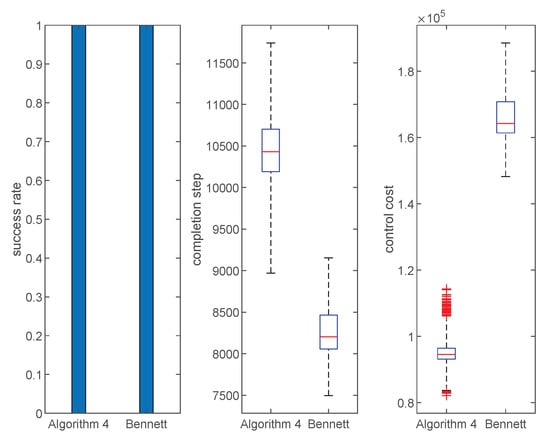
Figure 14.
Results comparing Algorithm 4 with Bennett’s Algorithm.
5.4. Parameter Analysis
In this subsection, we will examine how different parameters will affect the performance of the proposed algorithm. Since Algorithm 4 has integrated all the considerations, it is used as the test algorithm. By comprehensive numerical simulation, among all the design parameters, it is found that the variations of the following four parameters would make a drastic change in the algorithm performance, namely, , , , and . In this subsection, . The detailed analysis is as follows.
The algorithm performance with respect to the variations of is shown by Figure 15. As increases from to , both completion step and control cost decrease, where the biggest decrease happens when changes from to . determines when the sheepdog could change moving direction. For large , the sheepdog is more likely to meet the turning condition, and hence the route of the sheepdog is shortened, leading to less completion step and control cost as shown by Figure 15. On the contrary, when it is smaller, herding will fail.
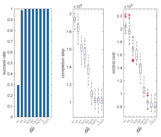
Figure 15.
The algorithm performance with respect to the variations of .
The algorithm performance with respect to the variations of is shown in Figure 16. For lower , the sheepdog moves too slowly that the herding task may not be successfully completed. Even if herding is achieved, the completion step is quite large, though at a rather low control cost. When varies from to , the completion step decreases initially and then becomes constant, while the control cost keeps increasing. Thus, if both the completion step and control cost is taken into consideration, the values for around might be a good choice.
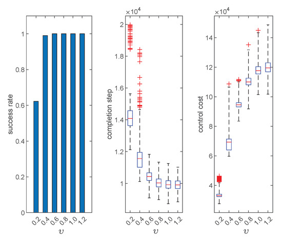
Figure 16.
The algorithm performance with respect to the variations of .
The algorithm performance with respect to the variations of is shown in Figure 17. For small detouring angle , the sheepdog tends to approach the critical sheep directly. As a result, it may get too close to the sheep herd, which may cause the sheep herd to oscillate along the directions of and , thus increasing the completion step. As increases, the oscillation is alleviated, and the control cost is also reduced. However, when further increases, the completion step almost remains the same, with a slight trend of increasing, but the control cost is increasing drastically. The reason is that for an overly large detouring angle , the sheepdog keeps a rather long distance from the sheep herd. Therefore, it probably takes more control costs to achieve herding.
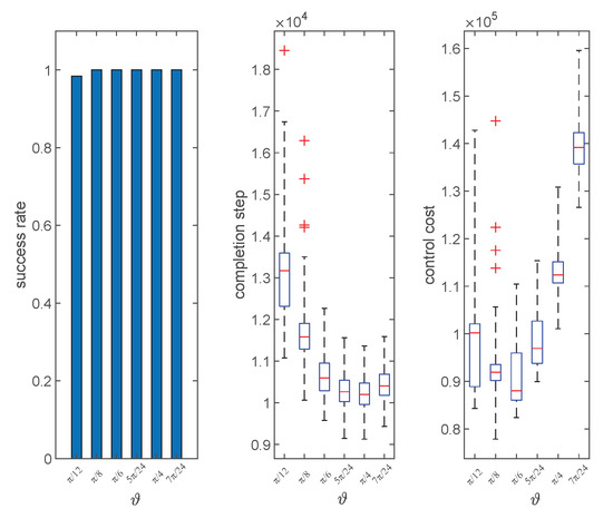
Figure 17.
The algorithm performance with respect to the variations of .
The algorithm performance with respect to the variations of is shown in Figure 18. determines when the sheepdog should pause. For large , the sheepdog pauses even if it is still quite far from the sheep herd, which greatly reduces the efficiency of the herding algorithm and also leads to a rather low success rate. If we reduce , then the sheepdog pause less, which, on the one hand, makes herding faster, and on the other hand, increases the control cost.
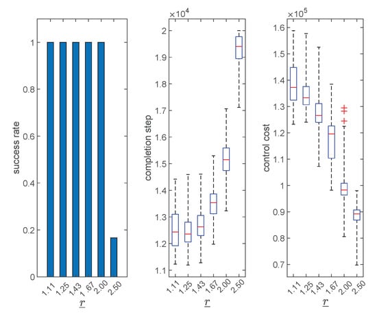
Figure 18.
The algorithm performance with respect to the variations of .
5.5. Size of the Sheep Herd
In this subsection, we will examine the performance of Algorithm 4 for different size of the sheep herd, namely, . Suppose the initial positions of the sheep are within the range of . Let and . The algorithm performance is shown in Figure 19. When the size of the sheep herd is small, i.e., , the scattering of the sheep herd and the weak attraction between sheep will increase the difficulty for the sheepdog to gather the sheep herd. That explains why it takes longer time to complete herding. When the size of the sheep herd is big, i.e., , the detouring distance of the sheepdog becomes longer, and the sheep at the forefront of the sheep herd will be less and less controllable by the sheepdog. In general, if the size of the sheep herd keeps increasing, it will take more and more time and control costs to herd.
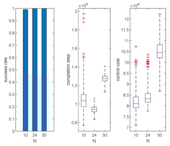
Figure 19.
The algorithm performance with respect to the variations of N.
6. Conclusions and Discussion
In this paper, for the social force model-based sheep herd, four behavior-based herding algorithms have been developed to solve the herding problem. By defining four critical sheep, a basic behavior-based herding algorithm is first proposed. Then, the dynamic far-end mechanism is synthesized to avoid the undesired circling behavior in the final stage of herding, and the pausing mechanism is conceived to reduce the control cost. It is shown by experiments that the circling issue would be more severe when the destination area becomes smaller. The simulation data have validated the effectiveness of the proposed herding algorithms. By Table 1, it can be further calculated that the integrated Algorithm 4 improves 23.7%, 0, 8.1% in terms of success rate; reduces −0.06%, −10.02%, 7.02% in terms of completion step and reduces 23.51%, 17.16%, 7.92% in terms of control cost compared to Algorithm 1, Algorithm 2, and Algorithm 3, respectively. Moreover, a thorough analysis has also been performed, discussing how the design parameters , , , and will affect the performance. Finally, we check the performance of Algorithm 4 for and 50. The results indicate that it will take more and more time and control costs to herd as the size of the sheep herd increases. Nevertheless, this work might still be improved from the following aspects. First, if the size of the sheep herd is greatly enlarged, then a single sheepdog would obviously be insufficient to deal with the herding problem. In such cases, it is necessary to consider the cooperation of multiple sheepdogs. Second, we have not considered obstacles or boundaries in this paper, which are common in practice. Besides completing the herding task in such a complex environment, it would be more interesting to think about how to make use of the specific conditions of the environment to help to herd.
Author Contributions
Conceptualization, H.C.; Methodology, H.C., Y.H., J.W. and H.G.; Software, J.W.; Validation, Y.H., J.W. and H.G.; Formal analysis, H.C., Y.H. and H.G.; Writing—original draft, H.C. and Y.H.; Funding acquisition, H.C. and H.G. All authors have read and agreed to the published version of the manuscript.
Funding
This research was funded in part by the National Natural Science Foundation of China under grant number 62173149, 62276104, and in part by the Guangdong Natural Science Foundation under grant number 2021A1515012584, 2022A1515011262.
Data Availability Statement
The data presented in this study are available on request from the corresponding author.
Conflicts of Interest
The authors declare no conflict of interest.
Nomenclature
| the position of the ith sheep at step k | |
| the velocity of the ith sheep at step k | |
| the position of the sheepdog at step k | |
| the velocity of the sheepdog at step k | |
| T | the sampling period |
| the relative position of the jth sheep towards the ith sheep | |
| the relative position of the sheepdog towards the ith sheep | |
| perceptive radius of the sheep | |
| perceptive radius of the sheepdog | |
| the label set of all the sheep visible to sheep i at step k | |
| the label set of all the sheep visible to the sheepdog at step k | |
| the center of the visible sheep set at step k | |
| the effect from other sheep to the ith sheep at step k | |
| the effect from the sheepdog to the ith sheep at step k | |
| noise | |
| the upper limit for the speed of sheep | |
| the sheep herd polygon at step k | |
| destination area | |
| the center of | |
| the radius of the destination area | |
| the direction of sheep herd towards destination area at step k | |
| the left vertical of | |
| the right vertical of | |
| the direction of the sheepdog towards the | |
| the left anchor sheep at step k | |
| the right anchor sheep at step k | |
| the left front sheep at step k | |
| the right front sheep at step k | |
| left turning angle at step k | |
| right turning angle at step k | |
| state flag at step k | |
| the upper limit of sheepdog’s speed | |
| the dynamic far-end at step k | |
| back declination angle of sheepdog relative to sheep herd at step k | |
| the approaching ratio at step k | |
| the allowable minimal distance between the sheep and the sheepdog | |
| the minimal sheep-to-sheep safety distance | |
| the maximal action distance of the repulsive effect between two sheep | |
| the minimal action distance of the attractive effect between two sheep | |
| the intensity coefficient of sheepdog-to-sheep repulsive force | |
| the intensity coefficient of sheep-to-sheep repulsive force | |
| the intensity coefficient of sheep-to-sheep attractive force | |
| back-declination-angle threshold | |
| turning-angle threshold | |
| pausing threshold | |
| approaching threshold | |
| velocity coefficient | |
| detouring angle | |
| K | step limit |
| success rate | |
| completion step | |
| control cost |
References
- Voelkl, B.; Portugal, S.J.; Unsöld, M.; Usherwood, J.R.; Wilson, A.M.; Fritz, J. Matching times of leading and following suggest cooperation through direct reciprocity during V-formation flight in ibis. Proc. Natl. Acad. Sci. USA 2015, 112, 2115–2120. [Google Scholar] [CrossRef] [PubMed]
- Karaboga, D. An Idea Based on Honey Bee Swarm for Numerical Optimization; Technical Report, Technical Report-tr06; Erciyes University, Engineering Faculty, Computer Engineering Department: Kayseri, Turkey, 2005. [Google Scholar]
- Lopez, U.; Gautrais, J.; Couzin, I.D.; Theraulaz, G. From behavioural analyses to models of collective motion in fish schools. Interface Focus 2012, 2, 693–707. [Google Scholar] [CrossRef] [PubMed]
- Aoki. A simulation study on the schooling mechanism in fish. Bull. Jpn. Soc. Sci. Fish. 1982, 48, 1081–1088. [Google Scholar] [CrossRef]
- Reynolds, C.W. Flocks, herds and schools: A distributed behavioral model. In Proceedings of the 14th Annual Conference on Computer Graphics and Interactive Techniques, Anaheim, CA, USA, 27–31 July 1987; pp. 25–34. [Google Scholar]
- Huth, A.; Wissel, C. The simulation of the movement of fish schools. J. Theor. Biol. 1992, 156, 365–385. [Google Scholar] [CrossRef]
- Huth, A.; Wissel, C. The simulation of fish schools in comparison with experimental data. Ecol. Model. 1994, 75, 135–146. [Google Scholar] [CrossRef]
- Wang, X.; Yadav, V.; Balakrishnan, S. Cooperative UAV formation flying with obstacle/collision avoidance. IEEE Trans. Control. Syst. Technol. 2007, 15, 672–679. [Google Scholar] [CrossRef]
- Azoulay, R.; Reches, S. UAV Flocks Forming for Crowded Flight Environments. In Proceedings of the 11th International Conference on Agents and Artificial Intelligence (ICAART 2019), Prague, Czech Republic, 19–21 February 2019; pp. 154–163. [Google Scholar]
- Cruz, D.; McClintock, J.; Perteet, B.; Orqueda, O.A.; Cao, Y.; Fierro, R. Decentralized cooperative control-a multivehicle platform for research in networked embedded systems. IEEE Control. Syst. Mag. 2007, 27, 58–78. [Google Scholar]
- Beaver, L.E.; Chalaki, B.; Mahbub, A.I.; Zhao, L.; Zayas, R.; Malikopoulos, A.A. Demonstration of a time-efficient mobility system using a scaled smart city. Veh. Syst. Dyn. 2020, 58, 787–804. [Google Scholar] [CrossRef]
- Albert, A.; Imsland, L. Survey: Mobile sensor networks for target searching and tracking. Cyber-Phys. Syst. 2018, 4, 57–98. [Google Scholar] [CrossRef]
- Bayındır, L. A review of swarm robotics tasks. Neurocomputing 2016, 172, 292–321. [Google Scholar] [CrossRef]
- Fiorelli, E.; Leonard, N.E.; Bhatta, P.; Paley, D.A.; Bachmayer, R.; Fratantoni, D.M. Multi-AUV control and adaptive sampling in Monterey Bay. IEEE J. Ocean. Eng. 2006, 31, 935–948. [Google Scholar] [CrossRef]
- Lodovisi, C.; Loreti, P.; Bracciale, L.; Betti, S. Performance analysis of hybrid optical–acoustic AUV swarms for marine monitoring. Future Internet 2018, 10, 65. [Google Scholar] [CrossRef]
- Schulz, A.; Grefenstette, J.; Adams, W. Robo-shepherd: Learning complex robotic behaviors. In Proceedings of the Robotics and Manufacturing: Recent Trends in Research and Applications Sixth International Symposium on Robotics and Manufacturing (ISRAM ’96), Montpellier, France, 28–30 May 1996; ASME Press: New York, NY, USA, 1996; pp. 763–768. [Google Scholar]
- Funge, J.; Tu, X.; Terzopoulos, D. Cognitive modeling: Knowledge, reasoning and planning for intelligent characters. In Proceedings of the 26th Annual Conference on Computer Graphics and Interactive Techniques, Los Angeles, CA, USA, 8–13 August 1999; pp. 29–38. [Google Scholar]
- Vaughan, R.; Sumpter, N.; Henderson, J.; Frost, A.; Cameron, S. Experiments in automatic flock control. Robot. Auton. Syst. 2000, 31, 109–117. [Google Scholar] [CrossRef]
- Jyh-Ming, L.; Bayazit, O.B.; Sowell, R.T.; Rodriguez, S.; Amato, N.M. Shepherding behaviors. In Proceedings of the IEEE International Conference on Robotics and Automation, ICRA ’04, New Orleans, LA, USA, 26 April–1 May 2004; Volume 4, pp. 4159–4164. [Google Scholar]
- Jyh-Ming, L.; Rodriguez, S.; Malric, J.; Amato, N.M. Shepherding Behaviors with Multiple Shepherds. In Proceedings of the 2005 IEEE International Conference on Robotics and Automation, Barcelona, Spain, 18–22 April 2005; pp. 3402–3407. [Google Scholar]
- Bennett, B.; Trafankowski, M. A comparative investigation of herding algorithms. In Proceedings of the Symposionum on Understanding and Modelling Collective Phenomena (UMoCoP), Birmingham, UK, 2–6 July 2012; pp. 33–38. [Google Scholar]
- Fujioka, K. Effective Herding in Shepherding Problem in V-formation Control. Trans. Inst. Syst. Control. Inf. Eng. 2018, 31, 21–27. [Google Scholar] [CrossRef][Green Version]
- Zhang, S.; Lei, X.; Duan, M.; Peng, X.; Pan, J. Herding a Flock Using A Distributed Outmost Push Strategy with Multi-Robot System; Springer: Cham, Swizterland, 2022. [Google Scholar]
- Song, H.; Varava, A.; Kravchenko, O.; Kragic, D.; Wang, M.Y.; Pokorny, F.T.; Hang, K. Herding by caging: A formation-based motion planning framework for guiding mobile agents. Auton. Robot. 2021, 45, 613–631. [Google Scholar] [CrossRef]
- Pierson, A.; Schwager, M. Bio-inspired non-cooperative multi-robot herding. In Proceedings of the 2015 IEEE International Conference on Robotics and Automation (ICRA), Seattle, WA, USA, 26–30 May 2015; pp. 1843–1849. [Google Scholar]
- Pierson, A.; Schwager, M. Controlling Noncooperative Herds with Robotic Herders. IEEE Trans. Robot. 2018, 34, 517–525. [Google Scholar] [CrossRef]
- Li, X.; Huang, H.; Savkin, A.V.; Zhang, J. Robotic Herding of Farm Animals Using a Network of Barking Aerial Drones. Drones 2022, 6, 29. [Google Scholar] [CrossRef]
- Chuang, Y.; D’orsogna, M.R.; Marthaler, D.; Bertozzi, A.L.; Chayes, L.S. State transitions and the continuum limit for a 2D interacting, self-propelled particle system. Phys. D: Nonlinear Phenom. 2007, 232, 33–47. [Google Scholar] [CrossRef]
- Romanczuk, P.; Bär, M.; Ebeling, W.; Lindner, B.; Schimansky-Geier, L. Active brownian particles. Eur. Phys. J. Spec. Top. 2012, 202, 1–162. [Google Scholar] [CrossRef]
- Sung, M. Controlling Flock Through Normalized Radial Basis Function Interpolation. In Proceedings of the 3rd International Conference on Intelligent Technologies and Engineering Systems (ICITES2014), Kaohsiung, Taiwan, 19–21 December 2014; Springer: Cham, Switzrland, 2016; pp. 445–451. [Google Scholar]
- Mehran, R.; Oyama, A.; Shah, M. Abnormal crowd behavior detection using social force model. In Proceedings of the 2009 IEEE Conference on Computer Vision and Pattern Recognition, IEEE, Miami, FL, USA, 20–25 June 2009; pp. 935–942. [Google Scholar]
- Romanczuk, P.; Schimansky-Geier, L. Swarming and pattern formation due to selective attraction and repulsion. Interface Focus 2012, 2, 746–756. [Google Scholar] [CrossRef] [PubMed]
- Liu, Y.; Li, X.; Lan, M.; He, Y.; Cai, H.; Gao, H. Sheepdog Driven Algorithm for Sheep Herd Transport. In Proceedings of the 2021 40th Chinese Control Conference (CCC), Shanghai, China, 26–28 July 2021; pp. 5390–5395. [Google Scholar]
Disclaimer/Publisher’s Note: The statements, opinions and data contained in all publications are solely those of the individual author(s) and contributor(s) and not of MDPI and/or the editor(s). MDPI and/or the editor(s) disclaim responsibility for any injury to people or property resulting from any ideas, methods, instructions or products referred to in the content. |
© 2023 by the authors. Licensee MDPI, Basel, Switzerland. This article is an open access article distributed under the terms and conditions of the Creative Commons Attribution (CC BY) license (https://creativecommons.org/licenses/by/4.0/).