Vehicle Classification Using Deep Feature Fusion and Genetic Algorithms

Abstract

Vehicle classification is a challenging task in the area of image processing. It involves the classification of various vehicles based on their color, model, and make. A distinctive variety of vehicles belonging to various model categories have been developed in the automobile industry, which has made it necessary to establish a compact system that can classify vehicles within a complex model group. A well-established vehicle classification system has applications in security, vehicle monitoring in traffic cameras, route analysis in autonomous vehicles, and traffic control systems. In this paper, a hybrid model based on the integration of a pre-trained Convolutional Neural Network (CNN) and an evolutionary feature selection model is proposed for vehicle classification. The proposed model performs classification of eight different vehicle categories including sports cars, luxury cars and hybrid power-house SUVs. The used in this work is derived from Stanford car dataset that contains almost 196 cars and vehicle classes. After performing appropriate data preparation and preprocessing steps, feature learning and extraction is carried out using pre-trained VGG16 first that learns and extracts deep features from the set of input images. These features are then taken out of the last fully connected layer of VGG16, and feature optimization phase is carried out using evolution-based nature-inspired optimization model Genetic Algorithm (GA). The classification is performed using numerous SVM kernels where Cubic SVM achieves an accuracy of 99.7% and outperforms other kernels as well as excels in terns of performance as compared to the existing works.

1. Introduction

The evolution of the modern era has had a significant impact on the automobile industry, which has progressed rapidly. Nowadays, vehicles of the same companies are being released with various colors, models, and physical attributes, making it difficult to differentiate them without having some prior knowledge about those models that makes developing a system that could perform vehicle classification an even bigger challenge. The emerging concept of smart cities relies on an intelligent traffic monitoring and classification system that could detect and surveil different vehicles for traffic rule obstruction, security, and emergency situations [1]. The ever-increasing demand, production and usage of vehicles of all kinds of makes, colors and models, it becomes very difficult for a human agent to perform vehicle monitoring, record keeping, surveillance and detection for any kind of obstruction [2]. Therefore, establishing an automated system that can discriminate between various vehicle types is necessary. A model like this could have applications in the area of security, smart traffic systems, self-driving vehicles for environmental understanding and collision avoidance, criminal activity reduction, and vehicle-type detection [3].

An intelligent traffic system could also assist in crime reduction and criminal activity tracking, given that most criminal activities involve the use of some kind of vehicle for movement. In such cases, vehicle data could be obtained from ITS (Intelligent Transport System) to help with criminal tracking [4]. The main focus and purpose of this work is to generate such an automated, self-contained and intelligent computerized vision-based system which could differentiate between various vehicle categories with up to the mark precision and accuracy. Such a system would have significant applications in traffic monitoring, smart cities traffic controlling, security and auto vehicle detection in drones and self-driving cars. Until now, many conventional and handcrafted means have been used for vehicle discrimination through color, vehicle structure, or model. This identification process produces decent results on the targeted data for which the approach is implemented, but its functionality becomes limited, and the accuracy of classification gets very low when the data perspective changes and varying data are used [5]. Therefore, the latest deep learning and machine learning models are being used for the development of such automatic traffic classification systems. The convolutional neural networks (CNNs) are widely used for this purpose; they can be trained on large datasets initially and then used for more narrowly defined tasks. These deep learning CNN models are much better for classification than the conventional handcrafted methods; they comprise a huge number of deep convolution layers that allow better and deeper learning about random datasets [6]. Considering all these prospects, the automated vehicle detection and classification to be in this work will be comprised on CNN model together with appropriate optimization and classification methods. In this paper, an amalgamation scheme, based on a genetic algorithm (GA) and pre-trained CNN VGG16, has been proposed for automated vehicle classification. The dataset used in the project comprises of five vehicle classes (i.e., bike, car, bus, truck, and helicopter) which are then resized to maintain uniformity in image dimension. Next, these images are given as input to the deep convolutional network namely, VGG16, to perform feature extraction and learning within its deep layers. The extracted features are optimized and reduced using GA that evolves in iterations and looks for the most concerned solution points based on priority and discards the others. The selected features are then passed on to the classification learner, where they are classified with multiple Support vector machine (SVM) classifier variations. The experimental results showed that the proposed model, using the linear SVM (LSVM) classifier, achieved an accuracy level of 97.8%, outperforming other kernels and previous works. In a nutshell, the main contributions of the proposed work include the following:

• The Stanford dataset contains images of 196 different vehicle classes captured in real time which makes it prone to various artifacts including imbalance scale, illumination variance, unbalancing among different dataset classes. These issues are sorted out using certain preprocessing steps to make the results better.
• Achieving the best results on limited data is always a challenge, but the proposed model does not focus on bulks of data rather a specific amount of well-prepared data.
• The deployment of pre-trained VGG16 on the vehicle data enhances results to a huge extent as compared to the standard handcrafted methods and custom-made deep models.
• GA optimizes features by keeping the most suitable ones and discarding the rest thus eliminating the computational burden and training time which makes the proposed model extremely fast in training and prediction.

The rest of the paper has been organized as follows. The related work has been discussed in Section 2. Section 3 presents a detailed description of the proposed methodology. The details about the experiments and results have been given in Section 4 and Section 5 concludes the paper.

2. Related Work

Previous studies have proposed different vehicle classification systems, depending on their datasets. Molina-Cabello et al. [7] used the dataset comprising cars, trucks, and bikes and sequences obtained from the next generation simulation (NGSIM) program provided by the highway authorities. Image visual quality was enhanced using single-image super-resolution and median filter transformation. AlexNet was employed for feature learning in this scheme. The classification phase was performed using various classifiers, including a multilayer perceptron, an SVM, a naïve Bayes (NB), decision trees, and random forests. The model achieved a maximum accuracy of 91.5%. Oh and Ritchie [8] proposed a vehicle classification method based on loop signatures, also known as “blades.” The signatures of different vehicles, including cars, pickup trucks, SUVs, and vans, were obtained manually through blade sensors that had been installed along various parkways; the dataset was categorized into five divisions, each division containing 60 vehicles. A probabilistic neural network (PNN) was employed, based on a Bayesian classifier for vehicle data classification. The proposed model was evaluated using the correct classification rate, in this case, 75%.

He, Shao, and Tan [9] used a dataset consisting of 1196 car images with a frontal perspective covering 30 standalone car models in 12 of their makes. Images were enhanced using illumination normalization and a multiscale retinex. A part-based detection model was used to segment various regions of the vehicles and parts by their importance, namely, headlights, logos, and grills, separated by using the ROIs (Region of Interests), making it easy to classify different models of the same vehicle. Local Binary Patterns (LBP) and Histogram of Oriented Gradients (HOG) feature extractors were used to extract geometrical and textural features from the defined image regions. The classification stage of proposed model was performed by various classifiers where the maximum detection accuracy was achieved by the AdaBoost classifier, proving out at 94.8%. Psyllos et al. [10] also used a frontal view vehicle image dataset for vehicle manufacturer and model recognition. The vehicle logos, license plates, and headlight grills were segmented using masking and Phase Congruency Detection. Feature extraction, learning, and classification were performed using a PNN comprising input, radial, and output layers that categorized the input patterns into pre-allocated classes. The proposed model achieved an accuracy of 94%. Sheng et al. [11] used the Stanford dataset and formulated six classes: Volkswagen, Audi, Chevrolet, BMW, Mercedes-Benz, and Ford. The work focused on the classification of vehicle type and area detection for a particular vehicle. The experiments were performed with six CNNs—AlexNet, VGG16, VGG19, GoogleNet, ResNet50, and ResNet101—for both an RCNN and a faster RCNN. The proposed model provided an average accuracy of 93.32% when discriminating six vehicle types.

Soon et al. [12] used a vehicle dataset BIT containing 9850 vehicle images in six vehicle categories: bus, minivan, microbus, sedan, SUV, and truck. Images were preprocessed to eliminate those showing more than one vehicle. The image count after preprocessing in each vehicle class was 558 buses, 883 microbuses, 476 minivans, 5922 sedans, 1392 SUVs, and 822 trucks. A novel principal component analysis (PCA) convolutional network was proposed in which the massive time consumption of the CNN was resolved by composing the convolutional layer filters of the CNN with the help of PCA. This process reduced the training burden and produced flexible features against various aspects. The proposed model yielded an average accuracy of above 88.35% in various conditions. Mundhenk et al. [13] compiled a Cars Overhead with Context (COWC) dataset containing 32,716 images from six image classes obtained from various geographic regions. A CNN named ResCeption was proposed, using AlexNet as a baseline and GoogleNet/Inception as a batch normalizer. The proposed model achieved an average accuracy of 97.294%.

Divyavarshini et al. [14] constituted a sutom CNN model comprising of 25 max pooling layers for vehicle type recignition. Feature extraction is performed by the proposed CNN model and also by the handcrafted HOG feature extractor. Resultant vectors from both the models are fused and classified using SVM classifier. Ahsan et al. [15] proposed a CNN-based model for vehicle number plate detection and processing. The model captures take the digital camera captured image and uses the super pixel resolution method to enhance the image quality. All the number plate embedded characters are segmented using the bounding boxes. The pre-trained Alexnet is then used to derive 4096 features from the segmented numbered images and a maximum detection accuracy of 98.2% is achieved.

Dai et al. [16] improved the pre-trained ResNet-50 model and formulated a faster R-CNN architecture for vehicle distance estimation and pedestrian estimation. Real time images are acquired using the infrared-based cameras which contained long distance roads containing pedestrians and tagged values. The model runs at the frame rate of 7 fps and provides an accuracy of 80% on the real time data.

Some of the recent works like [17,18,19] used for classification and detection of vehicles also motivated us to investigate deep learning techniques along with evolutionary techniques for intelligent transport system.

In contrast with the techniques mentioned above, we proposed an amalgamation scheme based on GA and pre-trained CNN VGG16 for automated vehicle classification. We used a deep convolutional network VGG16 for feature extraction and learning within its deep layers. The extracted features were optimized and reduced using a GA that evolved in iterations and looked for the most concerned solution points based on priority and discarded others. The selected features were then passed on to the classification learner, where they were classified with multiple SVM classifier variations.

3. Proposed Methodology

3.1. Deep Feature Fusion and Genetic Algorithms

Deep learning models have the tendency to extract the deep features from the input data given to them. These extracted features have complex dimensions, are in the form of vectors and contain most of the information derived from the input data. DL models can be of two types: pre-trained CNN models such as AlexNet, GoogleNet, ResNet150 etc. or custom CNN models. The pre-trained CNN models are already trained on massive amounts of data compilations and can therefore provide good results in in most cases. However, the customs CNN models need to be trained well before testing them on real datasets. There are certain cases in which even a single pre-trained model does not provide better results. This type of situation can happen when the data set is not well prepared there are multiple datasets involved. In such cases, it is better to merge the features learned by the two separate CNN models using the methods of transfer learning and feature fusion. The learned features are extracted from the last fully connected layers or pooling layers of respective CNN models are merged to formulate a compact vectorized feature vector combination. Later, when these merged features are provided to machine learning-based classifiers, a significant increase in the performance is observed in most of the cases. This future fusion can help increase the performance of the proposed model, but it leads to feature complexity and model entanglement. It is observed in most of the cases that model provides better results but at a cost of increased time after feature fusion. This causes the need for a feature selector or an optimization algorithm that may reduce the complexity of these fused features while maintaining the important details contained within them. Several nature-based evolutionary models as well as mathematically formulated feature optimization models exist out there that are used for such purpose. Genetic Algorithm (GA) is a metaheuristic algorithm inspired by the process of natural selection and it belongs to the larger class of evolutionary algorithms. It calculates high quality and global optimal solutions for against the problem space provided to it. It contains populations of individuals which are the possible solutions for given problem in a search space. These possible solutions, also termed as chromosomes spread in the problem space and find the nearest optimal solution while keeping the other chromosomes updated with their status. The chromosome nearest to the optimal solution is the best solution and is selected for problem solving, which is then reproduced by crossover process to generate its offspring. This process is followed by altering some of the genes in the mutation phase and finally the initial population is encoded. This process continues until all of the problem space is explored.

3.2. Proposed Work

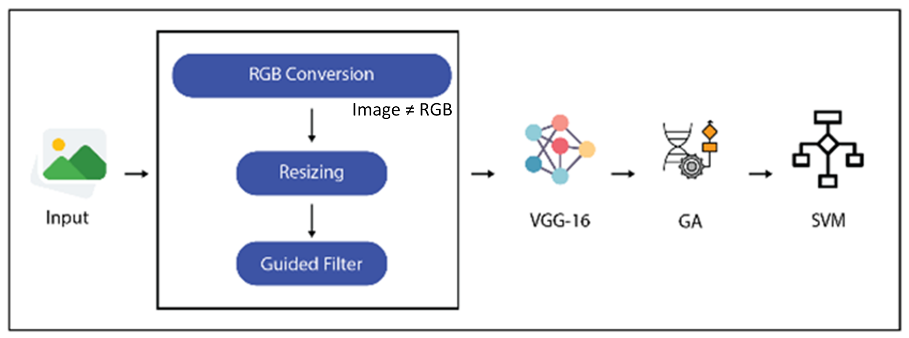
In the proposed work, a deep CNN and a natural evolution-based GA algorithm are combined to formulate an automated classification system for eight different vehicle categories. The model is initially composed of deep CNN VGG16 that uses its deep layers to perform feature extraction and learning. These features are extracted from the last fully connected layer of CNN and since these features are massive in number and may contain ambiguous information as well that affects results. Therefore, an evolutionary feature selector GA is employed to keep the most related features and discard others. The classification phase is performed with several SVM kernels to see which performs best on the current data nature. The proposed model workflow is illustrated in Figure 1.

3.3. Data Acquisition and Preprocessing

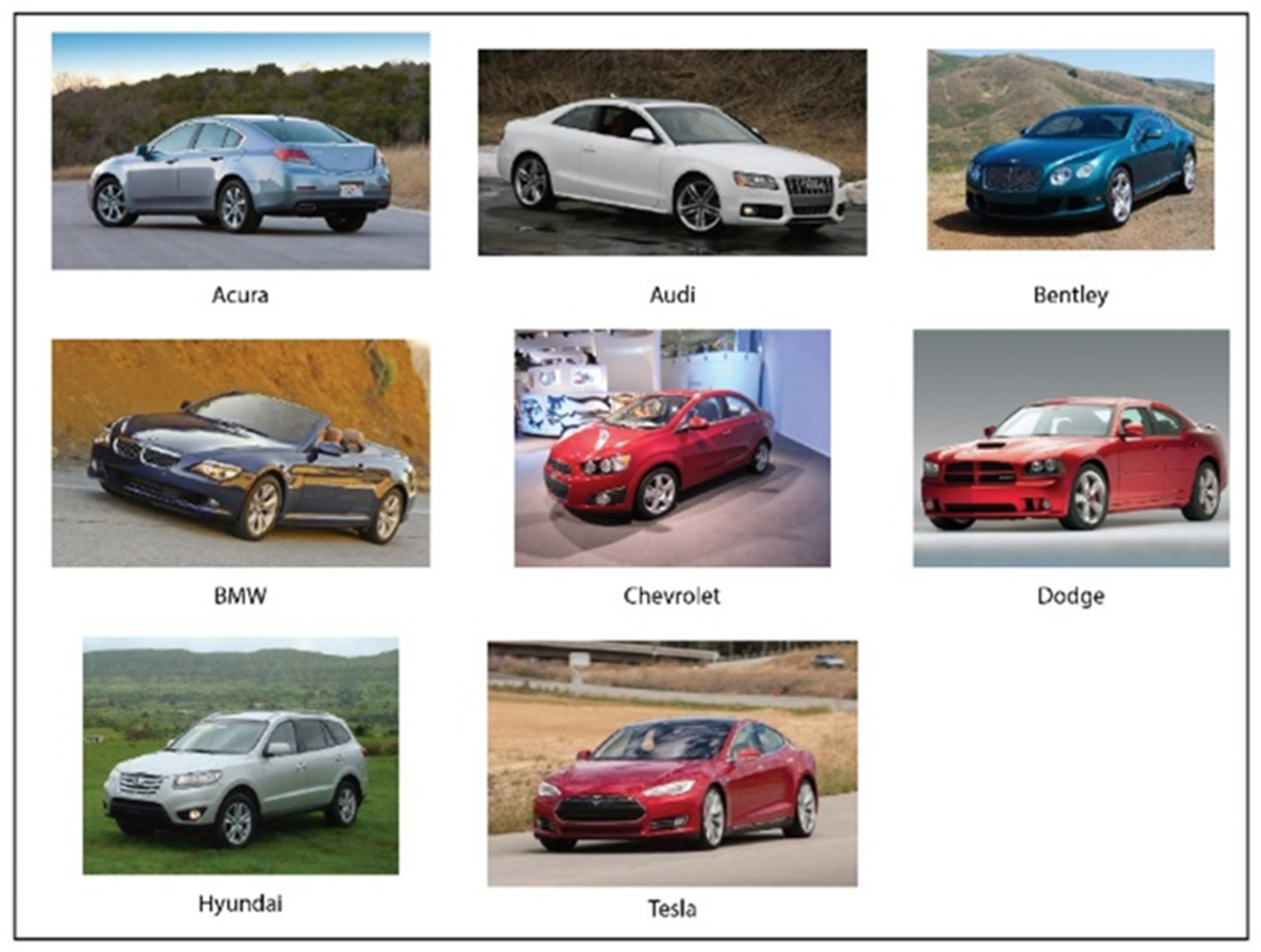
The dataset used in the proposed work is derived from the publicly available Stanford car dataset. The original dataset contains 196 different vehicles classes and over 8800 images. We only selected eight distinct vehicle classes each containing approximately 45 images. The selected vehicles classes are based on images from some of the famous brands including Acura, Audi, Bentley, BMW, Chevrolet, Dodge, Hyundai and Tesla. The dataset is passed through several augmentation steps including image flipping and rotation to increase the number of images in each class, balance the dataset classes and the post-augmentation dataset contains 1000 images per vehicle class. The final dataset contains a total of 8000 images divided among eight vehicle classes as shown in Figure 2.

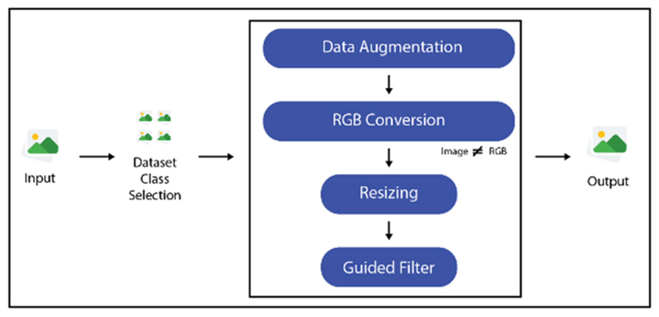
The images were also resized as VGG16 accepts images in dimension of 224 × 224 and to also create a uniformity among images so that the results are not affected by varying sizes. All the dataset images are resized into the dimensions of 224 × 224 before passing them on to feature extraction stage. Since Stanford dataset contains images that are captured in real-time through RGB cameras as well as black and white CCTV camera so some of the images are not in the RGB channel. Therefore, while preprocessing it is checked whether images are in RGB or some other color channel and those not in RGB are converted into RGB using RGB color map. In order to enhance the image quality and contrast, the Guided Filter is also applied. The preprocessing steps are elaborated in Figure 3.

3.4. Feature Extraction

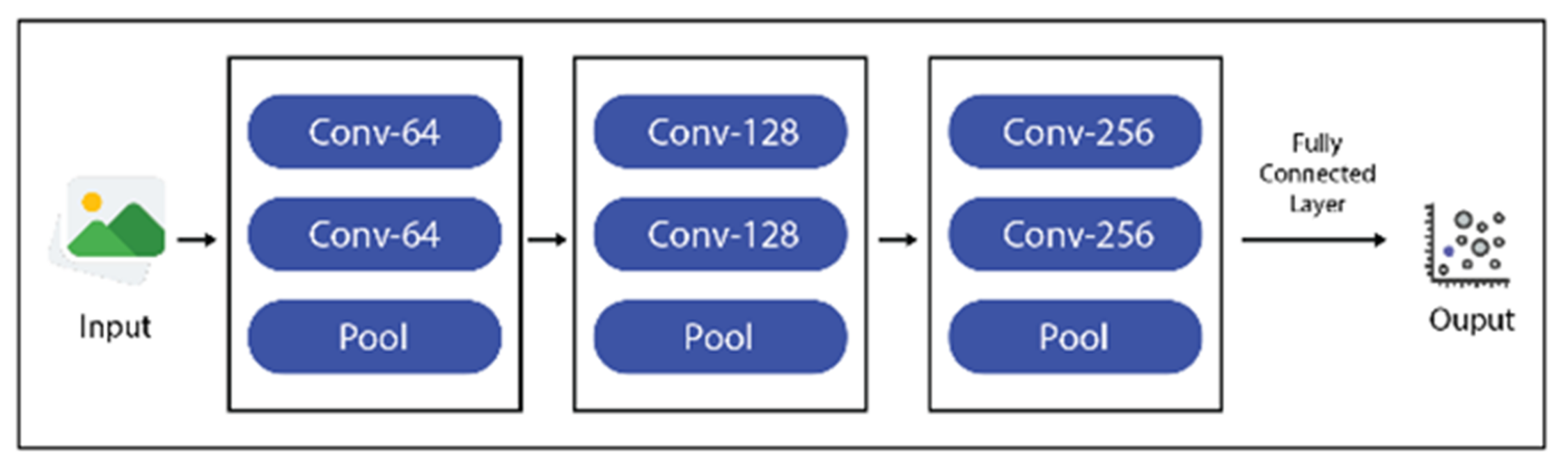
The resized images were passed on to the deep convolutional network model VGG16 for feature extraction and learning. VGG16 is a 16-layer-deep convolutional network trained on a massive ImageNet database and can discriminate among 1000 object categories. The input given to it was 224 × 224 (“VGG-16 Convolutional Neural Network-MATLAB VGG16” n.d.). It contains five combinations of convolutional layers in the form of batches, each containing 2 to 3 convolutional layers, followed by the pooling layers, as shown in Figure 4 [20].

A total of 8000 images were provided as input to the VGG16 model, that performed feature extraction using its deep layers. Images were provided as input to the VGG16 model, which performed the phases of feature extraction and learned on them in its deep layers.

Table 1. Overview of extracted features.

Model	Feature Layer	Images	Total Features
VGG16	fc8	8000	8000 × 1000

shows the details of the extracted features. The features were taken out of the last fully connected layer of the VGG16 model fc8; the SoftMax and classification layer were not used in this case; instead, the features were optimized first using the GA optimizer and then classified using the SVM classifier.

3.5. Feature Selection

The extracted features from the VGG16 model were obtained from its last fully connected layer, fc8, and were given as an input to the GA for optimization and reduction. GA calculated high-quality and globally optimal solutions for optimization problems. It contained populations of individuals based on chromosomes that were actually the possible solutions for a given situation in the search space. Each chromosome indicates a candidate solution and is further based on a list of variable values. A problem having $K_N$ number of possible solutions means that each chromosome will have a $K_N$ list as represented in Equation (1).

$$Chromosomes=[s_1,s_2,s_3,\cdots ,s_{K_N}],$$

(1)

where, each p represents possible solution with regard to a particular chromosome and there can be $S_{\left(K_N\right)}$ solutions. GA begins with selection of a random number of such chromosomes that actually serve as the agents in the initial iteration.

The process of finding optimal solution initiates and each population of chromosomes begin searching for solution in the declared search space. Each chromosome in the population maintains a certain fitness function as it searches for the problem in search space which is evaluated for all the chromosomes at the end of initial iteration. From a massive population containing chromosomes, some of the population is maintained based on the fitness scores of their chromosomes upon a user-defined probability while the rest is discarded. The fittest chromosomes are more likely to be chosen. The probability of a chromosome $C_{x}y$ to be selected considering g as a positive function is represented in Equation (2).

$$P\left(C_{xy}\right)=|\frac{g\left(C_{xy}\right)}{{\sum }_{a=1}^{N}g\left(C_k\right)}|,$$

(2)

where, $P\left(C_{xy}\right)$ represents the selection probability of a random chromosomes from the initial population, N represents total population, and $C_k$ represents the continuity of this function for the $k^{\mathrm{th}}$ number of chromosomes. The next phase comprises of crossover of the selected fittest chromosomes to increase the population of solution-finding agents. For this, a pair of chromosomes having the highest fitness score are chosen and offspring are generated from them. The crossover operation is demonstrated in Equation (3).

$$p_{cr}=\left\{{}_{p_{max-cr}{f}_x<f_{avg}}^{p_{max-cr}-\left(\frac{p_{max-cr}-p_{min-cr}}{T_n}\right)f_x\ge f_{avg}}\right\},$$

(3)

where, $p_{cr}$ is the crossover probability, $p_{max-cr}$ and $p_{min-cr}$ are the maximum and minimum crossover prospects, $T_n$ is the maximum possible iteration, $f_x$ is the chromosome with greatest fitness among the two chromosomes selected for crossover, and $f_{avg}$ denotes the overall fitness value of the whole population.

After the process of crossover, the final step of mutation is performed in which the genes of newly formulated offspring are altered with already available information to make them more effective. If this set of newly formed offspring provides with the optimal solution then the process is terminated otherwise this process is repeated till so.

For problem-solving, the best individual was selected in the GA, which was then reproduced by the crossover process to generate its offspring. This process was followed by altering some of the genes in the mutation phase and encoding the initial population [21].

Table 2. Feature selection overview for the proposed model.

Total Number of Extracted Features	Selected Features by GA
8000 × 1000	8000 × 500

shows the number features selected by GA. In this work, the number of chromosomes is kept at 10 , number of iterations is kept at 100, learning rate is 0.001. 80% of data is kept as training set and 20% data is kept as testing set for GA.

3.6. Classification

Finally, the selected features are transferred to the classification learner, where the classification phase is performed using the SVM classifiers together with its several kernel namely Linear SVM (L-SVM), Cubic SVM (CB-SVM), Quadratic SVM (Q-SVM), and Medium Gaussian SVM (MG-SVM). A total of 500 features which are selected by the GA from a set of 1000 deep model learned features are forwarded to these classifiers and each classifier is individually applied on them. The learning rate for the model is kept as 0.0001. The L-SVM classifier outperforms others in terms of accuracy. The proposed model performed better than the previous work in terms of both accuracy and time consumption, achieving an accuracy of 97.8%.

4. Experiments and Results

In the proposed work, a model was organized for the classification of vehicle images. The dataset used in the proposed work contains a total of 8000 images divided among eight vehicle classes. After data preparation and preprocessing, images were given to the pre-trained VGG16 for feature learning and extraction. The features were then extracted from the last fully connected layer of CNN and were then optimized using GA before passing them onto the SVM classifier.

The experiments were performed on Intel Core i7 with 8GB RAM and running on Windows 10 OS. The system houses a 256GB Solid State Drive (SSD) on which the MATLAB 2020a version is installed on which all the experiments are performed.

Table 3. Performance evaluation of classifiers used in the proposed model.

Kernel	Acc. (%)	Prec. (%)	Rec. (%)	F1 (%)	Tr. Time (s)
CB-SVM	99.88	99.875	99.875	99.875	100.5
L-SVM	85.25	85.25	85.375	85.125	106.39
Q-SVM	99.61	99.75	99.875	99.75	112.38
FG-SVM	96.8	96.625	97.5	97	416.05
MG-SVM	99.55	99.5	99.75	99.625	140.78
CG-SVM	69.14	69.125	69	69.125	287.06

shows the results of various SVM classifiers when directly applied on extracted features from CNN without optimization. The results are compared and evaluated with the help of evaluation measures precision, recall and f1-score. Cubic SVM stands out in terms of accuracy as compared to the rest of kernels, but a large amount of training time is compromised in this case. The goal here is to maintain the same performance rate but with significantly reduced time consumption since while conducting these experiments, a considerably better machine was used and even after that these kind of training times were encountered so time is only going to increase if the machine is not good enough and that is why optimization is so much needed.

The reason for CB-SVM being the best performing kernel is that CB-SVM performs best on non-linear features that are not easily differentiable via a hyperplane as it performs the same computation multiple times until the best results are achieved.

Table 4. Performance evaluation of classifiers used in the proposed model.

Kernel	Acc. (%)	Prec. (%)	Rec. (%)	F1 (%)	Tr. Time (s)
CB-SVM	99.71	99.75	99.75	99.875	31
L-SVM	84.66	84.75	84.875	84.625	27
Q-SVM	99.63	99.75	99.75	99.625	30
FG-SVM	97.01	97.125	97.625	97.875	65
MG-SVM	99.6	99.75	99.625	99.875	38
CG-SVM	69.14	69.125	69	69.125	52

shows the results of various SVM kernels when applied on GA-optimized features. The results are again compared using various performance measures as well as training time. When the results of Table 3 and Table 4 are compared, we have successfully achieved almost the same performance standards but with a greatly reduced time consumption rate. This makes our model stand out from the previous works as the proposed model provides the best results without compromising time.

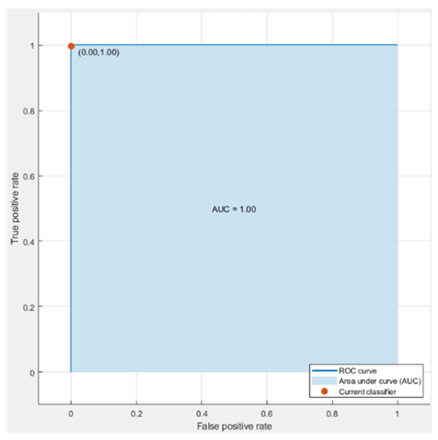
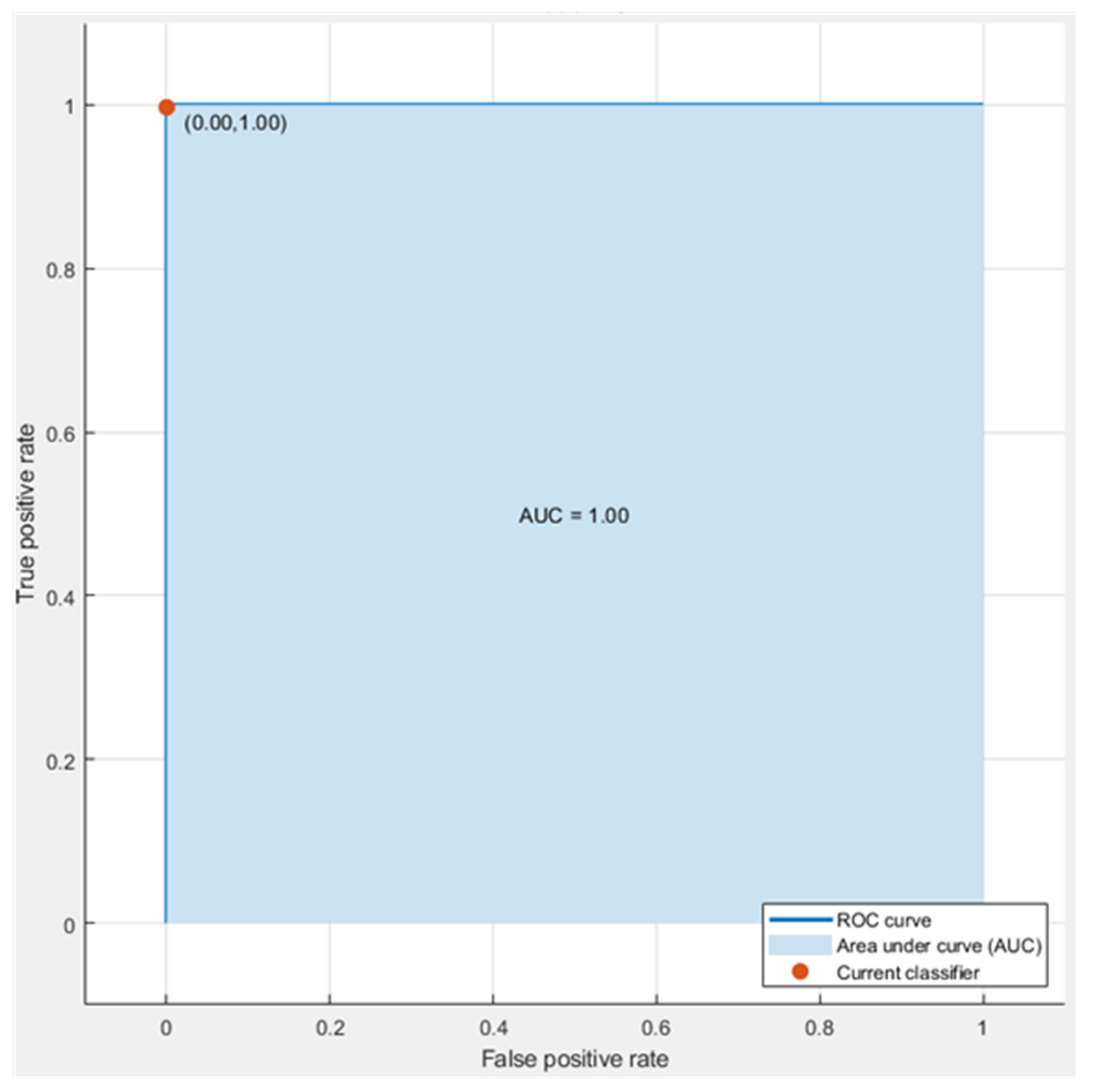
Figure 5 and Figure 6 show the ROC curves for Cubic SVM both when it classifies non-optimized and GA-optimized features. Also, Cubic SVM is the best performing model in both cases as evident from the tables above.

The ROC curve for the proposed model is illustrated in Figure 6, which shows that the area under the curve is exactly 1.00 while considering the true and false positive rates.

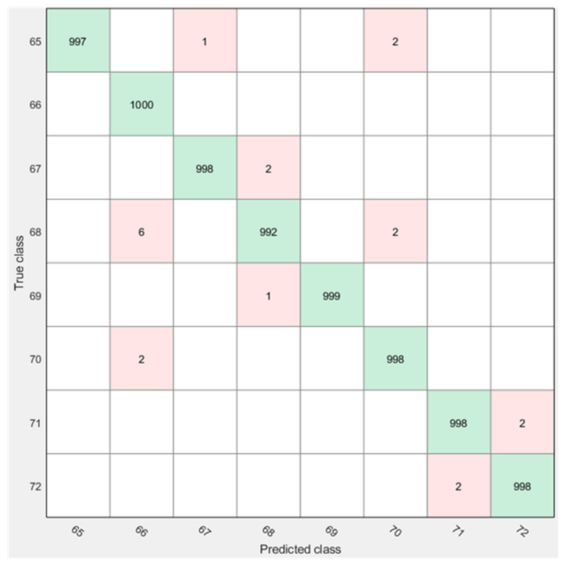
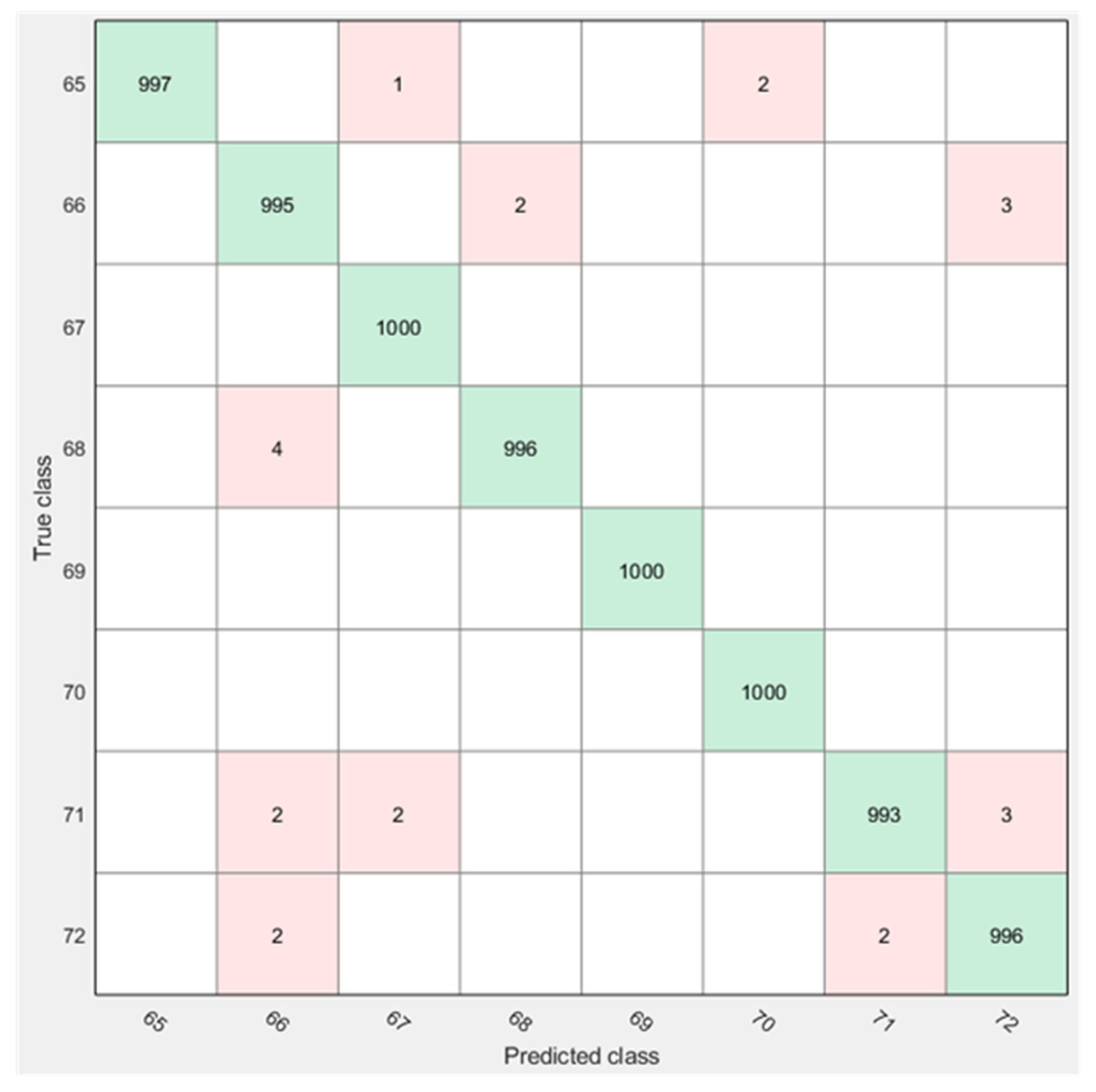
Similarly, Figure 7 and Figure 8 demonstrate confusion matrices for CB-SVM both for non-optimized and optimized features.

The reason behind extracting features from the last fully connected layer of VGG16 and using SVM to classify them is that former layer is followed by SoftMax and classification layers. The classification layer of a pre-trained VGG16 is programmed to classify 1000 different object classes. In this case, we only needed to classify eight vehicle classes, so the classification layer was not applicable. To make a fair comparison though, new SoftMax and classification layers were put in place and the extracted features were passed on to them straight after the “fc8” layer but the results were way behind.

The reason behind this is that the newly implanted layers need to be trained for massive data corpus just as the original VGG16’s layers have been trained on ImageNet database having 18 million images. But in this case, we are only going with 8000 images as achieving the best results with limited data is one of our targets of this research work and also that its not possible to train a CNN on such as massive dataset without having great computing resources. Therefore, the proposed model discards this approach and goes with the concerned approach.

Table 5. Proposed model and CNN classification accuracy comparison.

Proposed Model (Accuracy)	Vgg16 (Accuracy)
99.71%	28.80%

Shows the accuracy comparison between classification performed by the proposed model and the CNN. Table 5 shows the accuracy comparison of proposed model with CNN-based classification.

Figure 9 and Figure 10 demonstrated graphical visualization of the utilized SVM models in case of both non-optimized and optimized features.

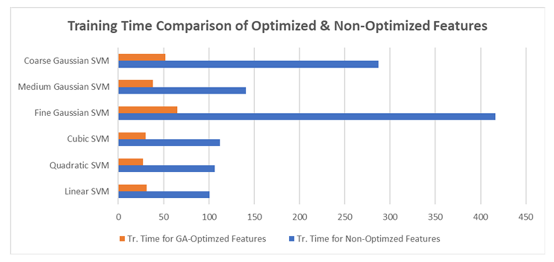
The proposed model has accomplished almost the same performance standards even after the implementation of GA and reduction of many features, but it also helped reduce time training time to a large extent. Figure 11 visualizes the difference between training time in the case of both the use cases.

Finally,

Table 6. Accuracy comparison with existing works.

Ref.	Year	Accuracy
[22]	2020	88%
[23]	2020	89.50%
[24]	2022	91.28%
[12]	2020	97.29%
Proposed	2022	99.78%

provides a comparison of the proposed model with the previously proposed works. The proposed model outperforms other works in terms of accuracy as well as time consumption rate.

Table 4 shows the overall statistics regarding the accuracy, training time, and prediction speed for the various SVM classifiers used in the classification phase. The LSVM classifier is chosen for the proposed model because it excels in both accuracy and prediction speed, with a slight trade-off for training time, which is negligible.

Table 6 shows a comparison of the proposed work with the latest studies presented in [22,23,24]. The proposed model outperformed the others in terms of accuracy and time management, providing the best accuracy as well as time efficiency.

5. Conclusions

An effective automated vehicle classification system based on the ideas of deep learning can assist in various real-world applications, including security, monitoring, and surveillance. A combination of deep CNN VGG16 and an evolution-based GA was proposed in this paper. In the proposed model, the feature learning was performed by VGG16 on a dataset containing eight vehicle classes. The feature selection was then performed by the GA. Finally, the classification was performed using the SVM classifier. The CB-LSVM classifier achieved an accuracy of 99.78%, which was better than the accuracy in previous studies. The proposed model excelled in both accuracy and time consumption, compared with those in previous studies. We believe that dataset can be increased largely and further work can be done to explore new pathways in the proposed work.