Longitudinal and Lateral Stability Control Strategies for ACC Systems of Differential Steering Electric Vehicles

Abstract

To ensure lateral stability during the cruising of a differential steering vehicle (DSV), this paper presents a curving adaptive cruise control (ACC) system coordinated with a differential steering control (DSC) system, which considers both longitudinal cruising capability and lateral stability on curved roads. Firstly, a DSV dynamics model is developed and a control strategy architecture for a curving ACC system is designed. Then, the car-following control strategy for the curving ACC system is designed based on the fuzzy model predictive control (FMPC) algorithm. The strategy aims to improve the economy and balances car following, safety, comfort and economy. Moreover, fuzzy logic rules are designed to update the weight coefficients of the performance indicators in real time. Finally, the lateral stability controller is designed based on the preview algorithm and the sliding mode control (SMC) algorithm. The simulation results show that the lateral stability of the DSV during the curving cruise is realized via the control of the differential drive torque of the two front wheels. The proposed FMPC controller and SMC controller based on the preview control algorithm satisfy the performance in terms of vehicle following and lateral stable driving in the process of cruising.

1. Introduction

At present, because of the rapidly increasing number of vehicles, traffic safety and congestion problems have become serious [1,2,3,4]. As a vehicle intelligent control system, ACC can help drivers avoid collision accidents and improve the active safety of vehicles [5,6]. Intelligent control systems can autonomously drive vehicles to achieve control objectives [7]. The ACC consists of longitudinal and lateral control. In the longitudinal direction, it controls the vehicle to cruise at a predetermined speed and maintain a safe distance from the preceding vehicle. In the lateral direction, it controls the vehicle to track over a predetermined trajectory. Due to the nonlinear characteristics of the ACC vehicle system, designing a reasonable control strategy to realize the longitudinal and lateral control of the vehicle is a problem that needs to be solved.

Car following performance is an important index to evaluate ACC system function. At present, many control algorithms are used to improve the longitudinal car-following performance of ACC systems. Mehdi et al. [8] designed an asymmetric car following model to improve following performance by controlling vehicle inter-distance, relative speed, and acceleration. Then, Guo et al. [9] further considered the vehicles in adjacent lanes and designed a merging prediction model to improve the following performance of vehicles by analyzing merging behavior in adjacent lanes. Yen et al. [10] designed a vehicle following model using a deep reinforcement learning algorithm, which reduced the number of unsafe followings and the number of inefficient vehicles. On the basis of ensuring car following performance, many studies have further considered the safety, comfort, and economy of the ACC system. Moon and Yi et al. [11,12], by analyzing the driver’s behavior, proposed a confusion matrix method to adjust the control parameters and designed an integrated ACC/CA system to ensure the safe driving of the vehicle. Seyed Mehdi et al. [13] proposed a novel reference signal for the ACC system, which reduced the time difference between the initial state and stable state, and improved comfort while ensuring safety. Based on reinforcement learning theory, Das et al. [14] improved traffic efficiency by controlling the parameters of the safe inter-distance model. Li et al. [15] proposed a lower-dimensional model predictive control (MPC) algorithm, which was applied to the design of the fuel economy controller of the ACC system to ensure the optimal control and fast response of the system. Although many studies have improved the following, safety, comfort, and economy of the ACC system, there is the problem of how to solve the contradictions between various performance indicators.

When ACC vehicles travel on curved roads, the control system needs to be able to control the vehicle both longitudinally and laterally [16,17]. Therefore, lateral stability should be considered in the design of the ACC system. Guo et al. [18] proposed the adaptive fuzzy control strategy to coordinate the longitudinal and lateral control of the vehicle to ensure stability and comfort. Zhang et al. [19] coordinated the ACC system with the direct yaw moment control (DYC) system, and used the robust constrained state feedback method to weaken the influence of the DYC on the ACC’s car following performance, and also improved its lateral stability. Li et al. [20] developed a control system that integrated ACC, rear steering control (RSC), and rollover braking control (RBC) to prevent the rollover index from exceeding the safety threshold, and it had better rollover stability in emergency situations. Many related studies integrated ACC and steer-by-wire (SBW) to ensure the stable driving of ACC vehicles [21,22]. As a kind of SBW and new type of steering mechanism, differential steering can generate different driving torques by controlling left and right wheels, which simplifies the complexity of the steering system [23,24]. It is usually applied to trajectory tracking control. For example, Chen et al. [25] used differential steering to track the desired front wheel steering angle, which could still have a good tracking effect when the vehicle-steering motor failed. Due to the difference between the differential steering mechanism and the traditional steering mechanism, if the cruise function of the ACC system needs to be realized, the control strategy needs to be redesigned for its special steering structure.

To further improve the economy and ensure the lateral stability of the vehicle on the basis of ensuring coordination among the following, safety, and comfort of the DSV during a curving cruise, a control strategy for the curving ACC system based on the DSV is proposed in this paper. Firstly, the dynamic model and prediction model of DSVs are established, and following, safety, comfort and economy are considered. Then, the performance indicators are designed, including a consideration of the cost function and I/O constraints, and the variable weight adjustment strategy is designed to maximize the cruising economy under the premise of ensuring safety. At the same time, the lateral stability control strategy is designed for the DSV, and the lateral stability is realized via the control of the differential driving torque of the front wheel. Finally, compared with the effect of MPC and DYC, the performance of the proposed the curving ACC system of the DSV is verified. In this paper, the ACC system and steer-by-wire technology are combined to ensure the lateral stability of the vehicle during curving cruising via the control of the front wheel’s differential torque. Meanwhile, fuzzy control rules are designed to improve vehicle economy.

The rest of this paper is organized as follows: The DSV dynamics models are presented in Section 2. Section 3 gives a detailed description about the design of the proposed FMPC algorithm. Section 4 gives a detailed description about the design of the proposed SMC algorithm of DSV based on preview control algorithm. Section 5 gives its performance as tested via a platform simulation. Section 6 contains the conclusions. The limitations of and future work resulting from this paper are described in Section 7.

2. Modeling of DSV

2.1. Dynamics Model of DSV

As a new form of steering adapted to vehicles driven by in-wheel motors (IWMs), differential steering needs to be modeled for the dynamics of IWM-driven vehicles with differential steering, so as to lay the foundation for further research on the dynamics control of differential steering. Figure 1 shows the three degrees of freedom (3-DOF) vehicle dynamics model.

The 3-DOF vehicle dynamics equations are expressed as follows:

$$\left\{\begin{array}{c}m\left({\dot{v}}_x-v_y\omega \right)=\left(F_{xfl}+F_{xfr}\right)\cos {\delta }_f+F_{xrl}+F_{xrr}-\left(F_{yfl}+F_{yfr}\right)\sin {\delta }_f\\ m\left({\dot{v}}_y+v_x\omega \right)=\left(F_{yfl}+F_{yfr}\right)\cos {\delta }_f+F_{yrl}+F_{yrr}+\left(F_{xfl}+F_{xfr}\right)\sin {\delta }_f\\ I_z\dot{\omega }=a\left(F_{yfl}+F_{yfr}\right)\cos {\delta }_f-b\left(F_{yrl}+F_{yrr}\right)+a\left(F_{xfl}+F_{xfr}\right)\sin {\delta }_f\end{array}\right.$$

(1)

where $F_{xfl}$, $F_{xfr}$, $F_{xrl}$, and $F_{xrr}$ are the longitudinal forces of the left front wheel, right front wheel, left rear wheel, and right rear wheel, respectively.

Considering that the wheel angle is small, since this paper only studies the front wheel’s differential steering, the rear wheel’s driving force is the same, so Equation (1) can be simplified as follows:

$$\left\{\begin{array}{c}m\left({\dot{v}}_x-v_y\omega \right)=\left(F_{xfl}+F_{xfr}\right)\cos {\delta }_f+F_{xrl}+F_{xrr}\\ m\left({\dot{v}}_y+v_x\omega \right)=F_{yfl}+F_{yfr}+F_{yrl}+F_{yrr}\\ I_z\dot{\omega }=a\left(F_{yfl}+F_{yfr}\right)-b\left(F_{yrl}+F_{yrr}\right)+\frac{l_s}{R}∆T\end{array}\right.$$

(2)

where $m$ is the vehicle mass, $v_x$ is the longitudinal speed, $v_y$ is the lateral speed, $l_s$ is the half of the front wheel distance, $R$ is the wheel rolling radius, $∆T$ is the front wheel’s drive torque difference, $I_z$ is the vehicle’s moment of inertia, $\omega$ is the yaw rate, and $a$ and $b$ are the distance from the front and rear axles to the center of mass, respectively.

Ignoring the rolling resistance and air resistance of the tire, the force analysis of each tire is carried out. The dynamic differential equations of the left front, right front, left rear and right rear wheel are as follows:

$$\left\{\begin{array}{c}{I}_{wfl}{\dot{\omega }}_{fl}=T_{fl}-F_{xfl}R\\ I_{wfr}{\dot{\omega }}_{fr}=T_{fr}-F_{xfr}R\\ I_{wrl}{\dot{\omega }}_{rl}=T_{rl}-F_{xrl}R\\ I_{wrr}{\dot{\omega }}_{rr}=T_{rr}-F_{xrr}R\end{array}\right.$$

(3)

where ${\omega }_{fl}$ is the rotating angular velocity of the left front wheel, ${\omega }_{fr}$ is the rotating angular velocity of the right front wheel, ${\omega }_{rl}$ is the rotating angular velocity of the left rear wheel, ${\omega }_{rr}$ is the rotating angular velocity of the right rear wheel, and $T_{fl}$, $T_{fr}$, $T_{rl}$ and $T_{rr}$ are the driving torques of the left front wheel, right front wheel, left rear wheel and right rear wheel, respectively.

Considering the same steering angle of the coaxial tire and the linear tire, the following applies:

$$\left\{\begin{array}{c}{\alpha }_f={\alpha }_{fl}={\alpha }_{fr}=-\beta -\frac{a\omega }{v_y}+{\delta }_f\\ {\alpha }_r={\alpha }_{rl}={\alpha }_{rr}=-\beta +\frac{b\omega }{v_y}\end{array}\right.$$

(4)

where ${\alpha }_{fl}$ and ${\alpha }_{fr}$ are the steering angles of the left wheel and right wheel of the front axle, respectively. ${\alpha }_{rl}$ and ${\alpha }_{rr}$ are the steering angles of the left wheel’s rear axle and the right wheel’s rear axle, respectively.

The structure of the differential steering system [26] is shown in Figure 2.

The dynamic equation of DSV can be expressed as follows [27]:

$$\left\{\begin{array}{c}{J}_e{\ddot{\delta }}_f+b_e{\dot{\delta }}_f=∆M+\tau -{\tau }_f\\ ∆M=\left(F_{xfr}-F_{xfl}\right)r_{\sigma }=\frac{r_{\sigma }}{R}∆T\end{array}\right.$$

(5)

where $J_e$ is the equivalent moment of inertia, $b_e$ is the steering damping, ${\tau }_f$ is the friction torque of the steering system, and $\tau$ is the aligning torque, which can be calculated as follows:

$$\left\{\begin{array}{c}\tau =k_1{k}_f{\alpha }_f\\ k_1=\frac{l^2}{3}\end{array}\right.$$

(6)

The dynamic equation of DSV [28] can be obtained by combining Equation (2) as follows:

$$\left\{\begin{array}{c}{\dot{\delta }}_f=-\frac{k_1{k}_f}{b_e}{\delta }_f+\frac{k_1{k}_f}{b_e}\beta +\frac{k_1{k}_{f}a}{v_x{b}_e}\omega +\frac{r_{\sigma }}{b_{e}R}∆T-\frac{J_e}{b_e}{\ddot{\delta }}_f\\ \dot{\beta }=\frac{F_{yfl}+F_{yfr}}{m{v}_x}+\frac{F_{yrl}+F_{yrr}}{m{v}_x}-\omega \\ \dot{\omega }=\frac{l_s}{I_{z}R}∆T+\frac{a\left(F_{yfl}+F_{yfr}\right)}{I_z}-\frac{b\left(F_{yrl}+F_{yrr}\right)}{I_z}\end{array}\right.$$

(7)

Since ${\ddot{\delta }}_f$ is very small and can be ignored in the actual calculation, the front wheel’s steering angle can be expressed as follows:

$${\dot{\delta }}_f=-\frac{k_1{k}_f}{b_e}{\delta }_f+\frac{k_1{k}_f}{b_e}\beta +\frac{k_1{k}_{f}a}{v_x{b}_e}\omega +\frac{r_{\sigma }}{b_{e}R}∆T$$

(8)

When ignoring the nonlinear problem of tires and assuming that the tire is linear, a linear vehicle model can be obtained, which is as follows:

$$\left\{\begin{array}{c}\dot{\delta }=\frac{k_1{k}_f}{b_e}\delta -\frac{k_1{k}_f}{b_e}\beta -\frac{k_1{k}_{f}a}{v_x{b}_e}\omega +\frac{r_{\sigma }}{b_{e}R}∆T\\ \dot{\beta }=-\frac{k_f+k_r}{m{v}_x}\beta +\left(\frac{b{k}_r-a{k}_f}{m{v}_x^2}-1\right)\omega +\frac{k_f}{m{v}_x}\delta \\ \dot{\omega }=\frac{b{k}_r-a{k}_f}{I_z}\beta -\frac{a^2{k}_f+b^2{k}_r}{I_z{v}_x}\omega +\frac{a{k}_f}{I_z}\delta +\frac{l_s}{I_{z}R}∆T\end{array}\right.$$

(9)

The state space equation is expressed as follows:

$$\dot{X}=AX+Bu$$

(10)

where $A=\left[\begin{array}{ccc}\frac{k_1{k}_f}{b_e}& -\frac{k_1{k}_f}{b_e}& -\frac{k_1{k}_{f}a}{v_x{b}_e}\\ \frac{k_f}{m{v}_x}& -\frac{k_f+k_r}{m{v}_x}& \frac{b{k}_r-a{k}_f}{m{v}_x^2}-1\\ \frac{a{k}_f}{I_z}& \frac{b{k}_r-a{k}_f}{I_z}& -\frac{a^2{k}_f+b^2{k}_r}{I_z{v}_x}\end{array}\right]$, $B=\left[\begin{array}{c}\frac{r_{\sigma }}{b_{e}R}\\ 0\\ \frac{l_s}{I_{z}R}\end{array}\right]$, $X=\left[\begin{array}{c}\delta \\ \beta \\ \gamma \end{array}\right]$, $u=\left[∆T\right]$.

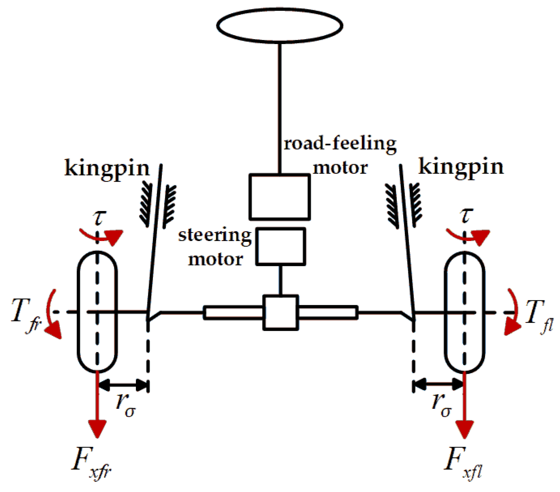
2.2. In-Wheel Motor Model

As the only power source of the DSV, the IWM needs to establish a more reasonable IWM model. Therefore, in this section, a suitable IWM is first selected as the drive motor of the DSV based on the limit values of the IWM parameters [29], and the IWM dynamics model is established.

The test parameters of DSV are shown in

Table 1. The DSV test parameters.

Vehicle Parameter	Definition	Value
$A_a$	wind area	2.8
$C_D$	coefficient of air resistance	0.35
$f$	coefficient of rolling resistance	0.012
$m$	vehicle mass	1830
${\delta }_c$	conversion coefficient of moment of inertia	1.3
$\eta$	total transmission efficiency of the drive system	0.94

.

According to the parameter matching of the vehicle power system, the maximum required power of the DSV during driving can be calculated. At the same time, in order to ensure that the 100 km acceleration time of the DSV equipped with the IWM meets the requirements of the vehicle performance index, it needs to be checked.

$$\left\{\begin{array}{c}{t}_T={\int }_0^{u_{rm}}\frac{{\delta }_{c}m}{3.6\left(-Gf+F_t-\frac{C_D{A}_a}{21.15}{u}_r^2\right)}d{u}_r\\ t_P={\int }_{u_{rm}}^{u_m}\frac{{\delta }_{c}m}{3.6\left(-Gf+F_t-\frac{C_D{A}_a}{21.15}{u}_r^2\right)}d{u}_r\\ u_{rm}=\frac{3.6\pi R{n}_m}{30}\\ F_t=\left\{\begin{array}{c}{T}_m/R\left(u_r\le u_{rm}\right)\\ T_P/R\left(u_{rm}\le u_r\le u_m\right)\end{array}\right.\\ T_P=\frac{9550P_m}{n}\\ t_1=t_T+t_P\end{array}\right.$$

(11)

where $u_{rm}$ is the speed of the motor at the rated speed, $u_m$ is the target speed, $u_r$ is the actual speed of the motor, $T_P$ is the output torque of the motor in a constant power range, and $t_T$ and $t_P$ are the acceleration time of the motor in the constant torque range and the constant power range, respectively. After calculation and verification, the acceleration time of the DSV is $t_1$ = 9.47 s, which meets the requirements of the vehicle dynamic performance index.

Based on the current motor control technology, this paper establishes the mathematical model of the IWM based on the principle of control theory and simplifies the model into a second-order response system [30], where the transfer function can be expressed as

$$G\left(s\right)=\frac{T_o}{T_{ox}}=\frac{1}{1+2\xi s+2{\xi }^2{s}^2}$$

(12)

where $T_o$ and $T_{ox}$ are the actual output torque and expected output torque of each IWM, respectively, and $\xi$ is the parameter-dependent damping ratio of the IWM, the value of which is 1.1.

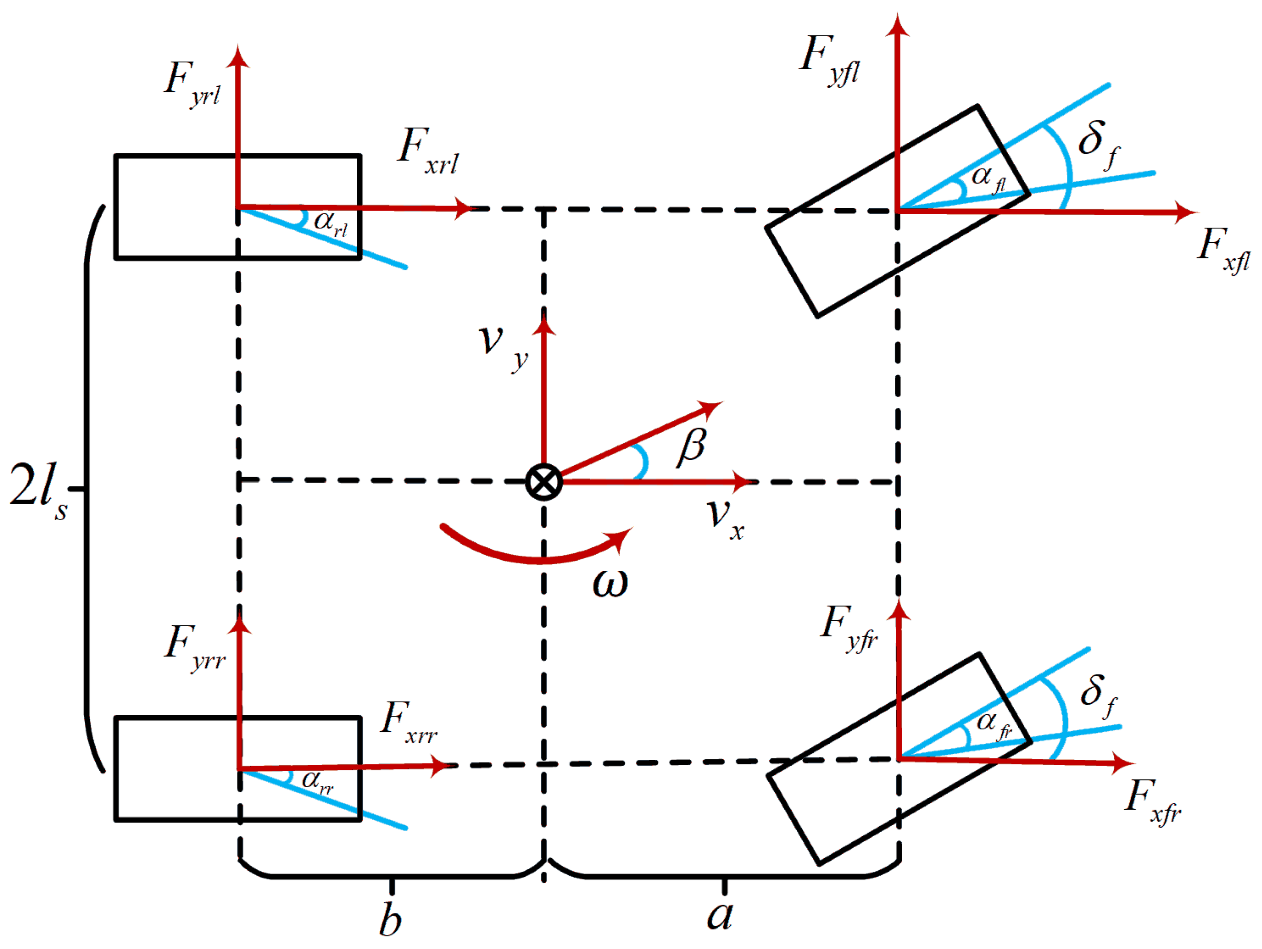
2.3. 2-DOF Vehicle Model

In this paper, a two degrees of freedom (2-DOF) vehicle model including the lateral motion of the vehicle along the y-axis and the yaw motion around the x-axis is used as a reference model, as shown in Figure 3.

The force balance equations of the vehicle reference model are as follows:

$$\left\{\begin{array}{c}\sum F_y=F_{yf}\cos {\delta }_d+F_{yr}\\ \sum M_z=a{F}_{yf}\cos {\delta }_d-b{F}_{yr}\end{array}\right.$$

(13)

where ${\delta }_d$ is the ideal front wheel’s steering angle calculated via preview control, and $F_{yf}$ and $F_{yr}$ are the sideslip forces of the front wheel and rear wheel, respectively.

When the front wheel steering angle of the DSV is relatively small, Equation (13) can be rewritten as follows:

$$\left\{\begin{array}{c}\sum F_y=k_f{\alpha }_f+k_r{\alpha }_r\\ \sum M_z=a{k}_f{\alpha }_f-b{k}_r{\alpha }_r\end{array}\right.$$

(14)

where $k_f$ and $k_r$ are the sideslip stiffness of the front wheels and rear wheels, respectively.

Suppose $\xi$ is the angle between $u$ and the x-axis, and ${\beta }_d=v/u$, the following applies:

$$\xi ={\beta }_d+\frac{a\omega }{u}$$

(15)

Combining Equations (4), (14) and (15), the differential equation of motion of the 2-DOF vehicle can be obtained, which is as follows:

$$\left\{\begin{array}{c}\left(k_f+k_r\right){\beta }_d+\frac{1}{u}\left(a{k}_f-b{k}_r\right)\omega -k_f{\delta }_d=m\left(\dot{v}+u\omega \right)\\ \left(a{k}_f-b{k}_r\right){\beta }_d+\frac{1}{u}\left(a^2{k}_f+b^2{k}_r\right)\omega -a{k}_f{\delta }_d=I_z\dot{\omega }\end{array}\right.$$

(16)

By changing the Laplace transform of Equation (16), the steady-state angular velocity gain can be obtained as follows:

$${\left(\frac{{\omega }_d}{{\delta }_d}\right)}_s=\frac{u/L}{1+\frac{m}{L^2}\left(\frac{a}{k_r}-\frac{b}{k_f}\right)u^2}=\frac{u/L}{1+K{u}^2}$$

(17)

According to Equation (17), the yaw rate when the vehicle is in steady state can be obtained as follows:

$$\left\{\begin{array}{c}{\omega }_d=\frac{u/L}{1+K{u}^2}{\delta }_d\\ K=\frac{m}{L^2}\left(\frac{a}{k_r}-\frac{b}{k_f}\right)\end{array}\right.$$

(18)

where $K$ is the stability factor.

The desired yaw rate is also related to road conditions.

$$a_y\le \mu g$$

(19)

where $\mu$ is the coefficient of road adhesion.

When the vehicle is in a uniform circular motion,

$$a_y=\frac{u^2}{R}={\omega }_{d}u$$

(20)

According to Formulas (19) and (20), the following can be obtained:

$${\omega }_d\le \frac{\mu g}{u}$$

(21)

Therefore, the desired yaw rate considering the road adhesion coefficient is

$${\omega }_d=min\left\{\left|\frac{u/L}{1+K{u}^2}\right|{\delta }_d,\left|\frac{\mu g}{u}\right|\right\}\times sgn\left(\frac{u/L}{1+K{u}^2}\right)$$

(22)

Similarly, according to Equation (16), the sideslip angle of the vehicle in a steady state can be obtained as follows:

$${\beta }_d={\delta }_d\left[\frac{b}{L\left(1+K{u}^2\right)}+\frac{u^{2}ma}{k_r{L}^2\left(1+K{u}^2\right)}\right]={\omega }_{d}u\left(\frac{b}{u^2}+\frac{ma}{k_{r}L}\right)$$

(23)

The desired sideslip angle considering the road adhesion coefficient can be obtained as follows:

$${\beta }_d\le {\omega }_{dmax}u\left(\frac{b}{u^2}+\frac{ma}{k_{r}L}\right)=\mu g\left(\frac{b}{u^2}+\frac{ma}{k_{r}L}\right)$$

(24)

Therefore, the desired sideslip angle considering the road adhesion coefficient is

$${\beta }_d=min\left\{\left|{\omega }_{d}u\left(\frac{b}{u^2}+\frac{ma}{k_{r}L}\right)\right|,\left|\mu g\left(\frac{b}{u^2}+\frac{ma}{k_{r}L}\right)\right|\right\}\times sgn\left[{\omega }_{d}u\left(\frac{b}{u^2}+\frac{ma}{k_{r}L}\right)\right]$$

(25)

In summary, the desired yaw rate and sideslip angle considering the road adhesion coefficient are as follows:

$$\left\{\begin{array}{c}{\omega }_d=min\left\{\left|\frac{u/L}{1+K{u}^2}\right|{\delta }_d,\left|\frac{\mu g}{u}\right|\right\}\times sgn\left(\frac{u/L}{1+K{u}^2}\right)\\ {\beta }_d=min\left\{\left|{\omega }_{d}u\left(\frac{b}{u^2}+\frac{ma}{k_{r}L}\right)\right|,\left|\mu g\left(\frac{b}{u^2}+\frac{ma}{k_{r}L}\right)\right|\right\}\times sgn\left[{\omega }_{d}u\left(\frac{b}{u^2}+\frac{ma}{k_{r}L}\right)\right]\end{array}\right.$$

(26)

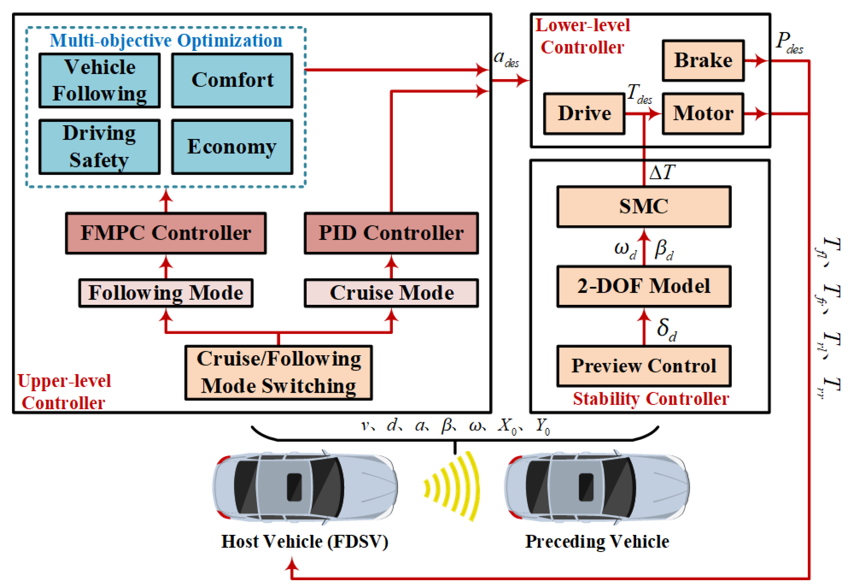
3. Control Strategy of Curving ACC System for DSV

3.1. The Framework of Curving ACC Control Strategy for DSV

Figure 4 shows the architecture of the ACC system control strategy of the DSV proposed in this paper on curved roads. The ACC system control strategy is made up of an upper-level controller, lower-level controller and lateral stability controller. Firstly, the upper-level controller selects the appropriate system working mode through the mode switching strategy according to the driving state of the two vehicles. For the cruise mode, a proportion integral differential (PID) control strategy is designed to obtain the desired acceleration. Aiming at the selection of the following mode, the upper-level control algorithm of the multi-objective ACC system with a variable weight is designed under the FMPC framework. Four performance indexes, following, safety, comfort and economy, are defined, and the constraints of the system are designed. The weights of following, comfort and economy are adjusted in real time to obtain the optimal acceleration.

Then, the lower-level controller converts the desired acceleration into the desired driving torque and braking pressure of the IWM through the inverse longitudinal dynamics model. For the DSV, a lateral stability controller is designed based on the SMC control algorithm, and the steering and stable driving of the vehicle are realized by calculating the differential driving torque of the front wheels.

3.2. The Upper-Level Control Strategy of the Cruise Mode

When the driver sets the cruising speed and starts cruise mode, the control strategy will calculate the desired acceleration of the DSV according to the actual speed measured by sensors, and output it to the lower-level controller, so that the actual acceleration can track the desired acceleration, in order to drive at the cruising speed set by the driver. The realization of the control algorithm of the cruise controller is relatively easy, so this paper will use the PID control algorithm to design the cruise controller.

Assuming that the driver’s preset cruise speed is $v_{hum}$, the speed of host vehicle is $v_f$, and the speed error is

$$e_1\left(t\right)=v_{hum}-v_f$$

(27)

In designing the upper-level controller for cruise mode based on PID control algorithm, the following applies:

$$u_1\left(t\right)=K_{P1}{e}_1\left(t\right)+K_{I1}\int e_1\left(t\right)dt+K_{D1}\dot{e_1}\left(t\right)$$

(28)

where $K_{P1}$, $K_{I1}$ and $K_{D1}$ are the proportional coefficient, integral coefficient and differential coefficient, respectively.

In this paper, the design parameters of the upper-level controller are tuned and adjusted, and finally determined as $K_{P1}=10$, $K_{I1}=0.01$, and $K_{D1}=0$. As a kind of ACC system working mode, the cruise mode is generally opened when the road conditions are good, there is no car in front, or the front car is far away. At the same time, comfort should be taken into account, so as to improve the acceptance and utilization rate of this working mode. According to the PID control principle, the desired acceleration will increase with the increase in the speed error, so it is necessary to limit the desired acceleration output from the PID controller. According to Payman Shakouri’s correlation analysis of the actual driving data and subjective evaluation, this paper sets the upper and lower limits of the desired acceleration as $2 \mathrm{m}/{\mathrm{s}}^2$ and $-4 \mathrm{m}/{\mathrm{s}}^2$, respectively.

3.3. The Upper-Level Control Strategy of the Following Mode

The inter-distance safety model is designed to provide a theoretical basis for the establishment of the upper-level control algorithm of the following mode of the ACC system of the DSV. Then, the objective function and constraints are established according to the four optimization objectives under the framework of the MPC, which are finally transformed into a quadratic programming solution problem with constraints [31]. Meanwhile, in order to ensure that the designed control algorithm can be adapted to the complex and changeable driving environment, according to the different focuses on different performance indicators, the weight coefficients in the objective function are updated in real time via fuzzy control on the basis of the MPC [32,33].

Assume that the state space expression for the linearized model of the discrete system is as follows:

$$\left\{\begin{array}{c}x\left(k+1\right)=f\left[x\left(k\right),u\left(k\right)\right]\\ y\left(k\right)=g\left[x\left(k\right),u\left(k\right)\right]\end{array}\right.$$

(29)

where $x\left(k\right)$ is the state variable, $y\left(k\right)$ is the output variable, and $u\left(k\right)$ is the control variable.

At the same time, it is necessary to optimize the error between the system output and reference variable and the system control variable to ensure that the objective function can make the controlled system track the desired reference trajectory quickly and smoothly [34], so the objective function often takes the following form:

$$J\left(k\right)=\sum _{i=1}^{N_p}{‖y_p\left(k+i|k\right)-r\left(k+i|k\right)‖}_Q^2+\sum _{i=0}^{N_c-1}{‖u_p\left(k+i|k\right)‖}_{R_r}^2$$

(30)

where $N_p$ is the prediction time domain, $N_c$ is the control time domain, $Q$ and $R_r$ are weight matrices, and $y_p\left(k+i|k\right)$ is the trajectory of the target vector of the performance metric to be optimized.

Considering the optimization objective and constraints, the optimization problem can be described as follows [35,36]:

$$\genfrac{}{}{0pt}{}{s.t.\left\{\begin{array}{c}{u}_{min}\le u_p\left(k+i|k\right)\le u_{max}\\ y_{min}\le u_p\left(k+i|k\right)\le y_{max}\end{array}\right.}{\min J\left(k\right)}$$

(31)

The above optimization problem is transformed into a quadratic programming problem that needs to satisfy both control constraints and output constraints to be solved to obtain the optimal control sequence.

$$U_k^{*}=\left\{u^{*}\left(k|k\right), u^{*}\left(k+1|k\right),\dots ,u^{*}\left(k+N_p-1|k\right)\right\}$$

(32)

3.3.1. Safety Inter-Distance Model

The safety inter-distance model is used as the distance input reference value of the upper-level controller of the ACC system, and the rationality of its design is the premise of ensuring the normal operation of the ACC system. In this paper, the safe inter-distance model of the ACC system is designed based on the constant time headway (CTH) algorithm and can be obtained via Equation (33), which lays a foundation for the design of subsequent control strategies.

$$d_{safe}={\tau }_h{v}_f+d_0$$

(33)

where ${\tau }_h$ is the time headway (THW), $v_f$ is the speed of preceding vehicle, and $d_0$ is the minimum holding inter-distance.

3.3.2. Longitudinal Kinematics Model

As shown in Figure 5 the longitudinal kinematic relationship of the vehicle of the ACC system is established.

The discrete state-space equations for the longitudinal kinematic model of the ACC system can be obtained as follows:

$$\left\{\begin{array}{c}x\left(k+1\right)=Ax\left(k\right)+Bu\left(k\right)+G\phi \left(k\right)\\ y\left(k\right)=Cx\left(k\right)-D\end{array}\right.$$

(34)

where $A=\left[\begin{array}{ccccc}1& 0& T_s& -\frac{T_s^2}{2}& 0\\ 0& 1& 0& T_s& 0\\ 0& 0& 1& -T_s& 0\\ 0& 0& 0& 1-\frac{T_s}{\tau }& 0\\ 0& 0& 0& -\frac{1}{\tau }& 0\end{array}\right]$, $B=\left[\begin{array}{c}0\\ 0\\ 0\\ \frac{T_s}{\tau }\\ \frac{1}{\tau }\end{array}\right]$, $C=\left[\begin{array}{ccccc}1& -{\tau }_h& 0& 0& 0\\ 0& 0& 1& 0& 0\\ 0& 0& 0& 1& 0\\ 0& 0& 0& 0& 1\end{array}\right]$, $D=\left[\begin{array}{c}{d}_0\\ 0\\ 0\\ 0\end{array}\right]$, $G=\left[\begin{array}{c}\frac{1}{2}{T}_s^2\\ 0\\ T_s\\ 0\\ 0\end{array}\right]$, $y\left(k\right)=\left[\begin{array}{c}∆d\left(k\right)\\ v_{rel}\left(k\right)\\ a_f\left(k\right)\\ jerk\left(k\right)\end{array}\right]$.

Define $x\left(k\right)={\left[d\left(k\right),v_f\left(k\right),v_{rel}\left(k\right),a_f\left(k\right),jerk\left(k\right)\right]}^T$; $d\left(k\right)$ is the actual distance, $v_f\left(k\right)$ is the speed of host vehicle, $v_{rel}\left(k\right)$ is the relative speed, $a_f\left(k\right)$ is the acceleration of the host vehicle, $jerk\left(k\right)$ is the host vehicle’s acceleration change rate, $u\left(k\right)$ is the desired acceleration of the host vehicle, $\phi \left(k\right)$ is the systematic disturbance, and $∆d\left(k\right)$ is the error of the inter-distance.

Considering the problem of multiple conflicting performance indexes, the hard constrains of the system are determined as follows:

$$\left\{\begin{array}{c}d\left(k\right)\ge d_0\\ v_{fmin}\le v_f\left(k\right)\le v_{fmax}\\ a_{fmin}\left(k\right)\le a_f\left(k\right)\le a_{fmax}\left(k\right)\\ {jerk}_{min}\le jerk\left(k\right)\le {jerk}_{max}\\ u_{min}\le u\left(k\right)\le u_{max}\end{array}\right.$$

(35)

The predicted state quantities of the longitudinal kinematic model of the ACC system are corrected using the prediction error $e\left(k\right)$ to improve the accuracy and precision of the prediction, and the predicted state quantities at the moment, $k$, are

$$x_p\left(k+1|k\right)=Ax\left(k\right)+Bu\left(k\right)+G\phi \left(k\right)+We\left(k\right)$$

(36)

where $W=diag\left(w_1,w_2,w_3,w_4,w_5\right)$ is the correction matrix, and each element of the $W$ species takes values in the range (0, 1).

According to the demand of control constraints for different constraints [37,38], the individual hard constraints are relaxed and adjusted to expand the range of the upper- and lower-bound constraints on the inputs and outputs of the system.

$$\left\{\begin{array}{c}d\left(k\right)\ge d_0+{\epsilon }_1{\xi }_{min}^d\\ v_{fmin}+{\epsilon }_2{\xi }_{min}^{v_f}\le v_f\left(k\right)\le v_{fmax}+{\epsilon }_2{\xi }_{max}^{v_f}\\ a_{fmin}+{\epsilon }_3{\xi }_{min}^{a_f}\le a_f\left(k\right)\le a_{fmax}+{\epsilon }_3{\xi }_{max}^{a_f}\\ {jerk}_{min}+{\epsilon }_4{\xi }_{min}^{jerk}\le jerk\left(k\right)\le {jerk}_{max}+{\epsilon }_4{\xi }_{max}^{jerk}\\ u_{min}+{\epsilon }_5{\xi }_{min}^u\le u\left(k\right)\le u_{max}+{\epsilon }_5{\xi }_{max}^u\end{array}\right.$$

(37)

where ${\epsilon }_i$ is the relaxation factor, ${\xi }_{max}^d$, ${\xi }_{max}^{v_f}$, ${\xi }_{max}^{a_f}$, ${\xi }_{max}^{jerk}$, ${\xi }_{max}^u$ is the relaxation coefficient of the upper bound of the hard constraint, and ${\xi }_{min}^{v_f}$, ${\xi }_{min}^{a_f}$, ${\xi }_{min}^{jerk}$, ${\xi }_{min}^u$ is the relaxation coefficient of the lower bound of the hard constraint.

3.3.3. Scrolling Optimization

According to the analysis of the system to be optimized and its objective function, the performances of vehicle following, passenger comfort, driving economy and driving safety are considered comprehensively under the MPC framework [39,40]; it is ensured that the DSV can quickly and smoothly track the preceding vehicle, and then the objective function is determined.

$$\begin{array}{c}J={\displaystyle \sum _{i=1}^{N_p}}{\left[y_p\left(k+i|k\right)-y_{ref}\left(k+i|k\right)\right]}^{T}Q\left[y_p\left(k+i|k\right)-y_{ref}\left(k+i|k\right)\right]\\ +{\displaystyle \sum _{i=1}^{N_p}}{u\left(k+i\right)}^T{R}_{r}u\left(k+i\right)\end{array}$$

(38)

where $y_{ref}\left(k+i|k\right)$ is the reference trajectory of the target vector of the performance metric to be optimized.

By deriving the objective function and constraints, the DSV multi-objective ACC cruise longitudinal following control algorithm is finally transformed into a quadratic programming solution problem with constraints.

$$\left\{\begin{array}{c}min\left\{{\tilde{U}}^{T}H\tilde{U}+2f\tilde{U}\right\}\\ \tilde{U}={\left[U,\epsilon \right]}^T\\ s.t. A_H\tilde{U}\le b_u\end{array}\right.$$

(39)

where $U$ is the set of control variables, $\epsilon$ is the vectorial relaxation factor, $A_H$ is the coefficient matrix of constraints, and $b_u$ is the constant term matrix of constraints.

From the MPC theory, the system will take the first component of the control sequence, $u^{*}\left(k\right)$, as the actual control input. The ACC decision algorithm will continue to predict and optimize the solution. The process is repeated continuously to achieve rolling optimized online control in the MPC framework.

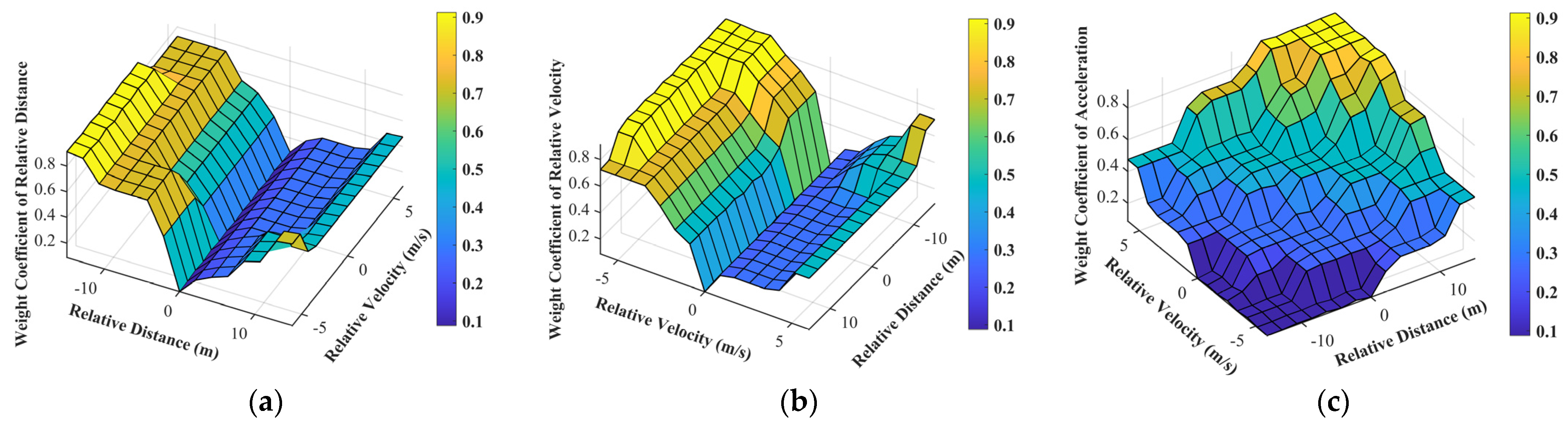
3.3.4. Variable Weight Coefficient Design Based on Fuzzy Control

The cost function of the system is as follows:

$$J=q_{∆d}{∆d}^2+q_{v_{rel}}{v}_{rel}^2+q_{a_f}{a}_f^2+q_{jerk}{jerk}^2$$

(40)

The method of fuzzy logic is used to establish the ACC system MPC controller’s cost function weight coefficient adjustment system, and the control algorithm system framework diagram is shown in Figure 6.

The values of the fuzzy linguistic variables of $∆d$, $v_{rel}$, $q_{∆d}$, $q_{v_{rel}}$, and $q_{a_f}$ are

$$\left\{\begin{array}{c}∆d,v_{rel} : \left\{NB,NM,NS,ZO,PS,PM,PB\right\}\\ q_{∆d},q_{v_{rel}},q_{a_f} : \left\{VS,S,M,B,VB\right\}\end{array}\right.$$

(41)

where $NB,NM,NS,ZO,PS,PM,PB$ represent negative big, negative medium, negative small, zero, positive small, positive medium and positive big, respectively. Meanwhile, $VS,S,M,B,VB$ represent negative small, small, medium, big and negative big, respectively. Set the fuzzification range of $∆d$ to $\left[-30, 30\right]$ m; $v_{rel}$ is limited to $\left[-12, 12\right]$ m/s. At the same time, the changes in areas of $q_{∆d}$, $q_{v_{rel}}$, and $q_{a_f}$ are set as $\left[0, 1\right]$.

The affiliation function is set in MATLAB Fuzzy Tool to create $q_{∆d}$, $q_{v_{rel}}$, and $q_{a_f}$ fuzzy rules as shown in Figure 7, respectively.

As shown in Figure 7a, we can see that when the relative distance is negative, the host vehicle easily collides with the preceding vehicle, and the weight factor $q_{∆d}$ of $∆d$ should be increased quickly to ensure that the host vehicle is safe. As the relative distance, $∆d$, increases, the degree of control over the distance can be reduced. In turn, when the relative distance is too far, we can control the relative distance to prevent excessive distance. From Figure 7b, it can be seen that when the relative velocity is negative, the velocity of the host vehicle is greater than the preceding vehicle, and if $∆d<0$, the host vehicle needs to slow down sharply. If $v_{rel}<0$ and $∆d>0$ occur at the same time, the host vehicle can slow down slowly to improve driving economy. For the weighting coefficient of acceleration in Figure 7c, when the host vehicle is in a dangerous situation, $q_{a_f}$ should be reduced in order for the host vehicle to be able to react quickly, and when the host vehicle is in a safe state, $q_{a_f}$ is increased, so that the host vehicle accelerates slowly, brakes slowly and improves the driving economy.

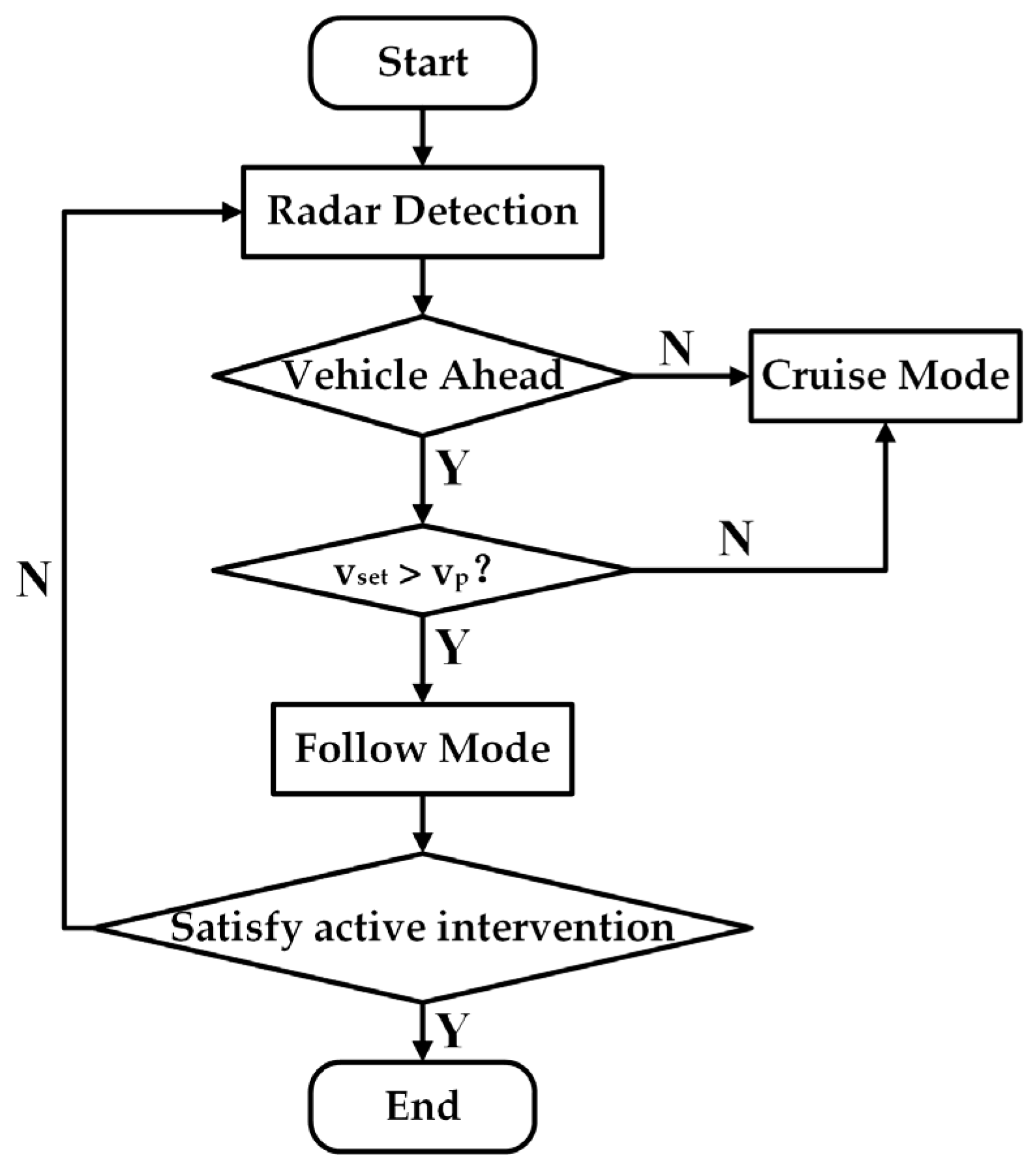
3.4. Mode Switching Logic of Curving ACC System for DSV

Figure 8 is the logic flow chart of cruise mode and following mode switching designed in this paper. At the same time, the following principles should be met during the driving process:

• The ACC system detects whether or not there is a preceding vehicle through the sensor, and the driver pre-sets the desired cruising speed. If the sensor does not detect the preceding vehicle, the ACC system will switch to the cruise mode for the speed to reach the desired driving speed. On the contrary, further judgment is needed;
• If the preceding vehicle’s speed,$v_p$, is detected as less than the cruise speed, $v_{set}$, the ACC system will switch to the following mode. On the contrary, it will enter or maintain the cruise mode;
• In the actual driving process, the ACC, as an auxiliary driving system, must follow the driver’s instruction priority principle. If the driver encounters an emergency during the driving process, the ACC system should immediately terminate the work and wait for the driver’s activation instructions when the driver has a mandatory operation.

3.5. The Lower-Level Control Strategy of the Curving ACC System

According to the construction of the DSV, when the DSV is accelerating, the torque generated by the motor is transferred to the wheels, which generates the corresponding driving torque to accelerate the vehicle. When the vehicle is decelerating, the braking pressure makes the braking system generate the corresponding braking force to decelerate the vehicle [41]. In this paper, we will establish a driving force and braking force calculation model based on the longitudinal dynamics model of the vehicle, establish an inverse longitudinal dynamics model of the vehicle according to the above principle, and convert the desired acceleration into the in-wheel motor torque and brake pressure signals.

3.5.1. Driving Model

Assuming that the vehicle is traveling on a flat and windless road and the air density is kept constant, the equation of vehicle travel can be obtained based on the driving force and driving resistance.

$$F_t=F_a+F_w+F_f+F_i$$

(42)

where $F_t$ is the driving force, $F_b$ is the braking force, $F_a$ is the acceleration resistance, $F_w$ is the air resistance, $F_f$ is the rolling resistance, and $F_i$ is the slope resistance.

$$\left\{\begin{array}{c}{F}_a={\delta }_{1}ma\\ F_w=\frac{C_D{A}_a{v}_f^2}{21.15}\\ F_f=mgf\\ F_i=mg\sin \theta =0\end{array}\right.$$

(43)

where ${\delta }_c$ is the conversion coefficient of vehicle’s rotating mass, $C_D$ is the coefficient of air resistance, $A_a$ is the frontal area, and $f$ is the coefficient of rolling resistance.

Since the IWM-driven electric vehicle is in a direct drive form, the transmission system is omitted, and the chassis structure is simplified. Therefore, according to Equations (42) and (43), the total desired driving torque of IWM, $T_{des}$, can be calculated as follows:

$$T_{des}=\left({\delta }_{c}ma+\frac{C_D{A}_a{v}_f^2}{21.15}+mgf\right)R$$

(44)

3.5.2. Braking Model

In the process of vehicle braking, part of the braking is provided by air resistance, rolling resistance and acceleration resistance, and excess braking is provided by the brake. According to the longitudinal dynamic equation of the vehicle, it can be expressed as follows:

$$a_a=\left(\frac{C_D{A}_a{v}_f^2}{21.15}+mgf\right)/{\delta }_{c}m$$

(45)

where $a_a$ is the acceleration in acceleration resistance.

The desired braking pressure is

$$P_{des}=\frac{{\delta }_{1}mR\left[a_{des}-\left(\frac{C_D{A}_a{v}_f^2}{21.15}+mgf\right)/{\delta }_{c}m\right]}{2\left(K_f+K_r\right)}$$

(46)

where $K_f$ and $K_r$ are the brake coefficients.

3.5.3. Design of Lower-Level Controller Based on PID

The longitudinal dynamics system of vehicle is a complex nonlinear system, the change of its parameters and the interference of the external environment have a large impact on the system, and the established inverse longitudinal dynamics model has the disadvantage of poor robustness, which cannot be fully adapted to the complex driving environment. Therefore, based on the inverse longitudinal dynamics model, this paper improves the response speed of the system by calculating the desired motor torque and braking pressure, and the error between the desired acceleration and the actual acceleration quickly tends to zero through the PID feedback control, so as to ensure the accuracy and robustness of the system.

According to the PID control theory, it can be obtained as follows:

$$e_2\left(t\right)=a_{des}\left(t\right)-a_f\left(t\right)$$

(47)

and the control model is obtained as follows:

$$u_2\left(t\right)=K_{P2}\times e_2\left(t\right)+K_{I2}\int e_2\left(t\right)dt+K_{D2}\times {\dot{e}}_2\left(t\right)$$

(48)

3.6. Verification of Simulation Results

The FHWA road is used to verify the control effect of the designed FMPC in this paper. The simulation parameters are shown in

Table 2. Table of simulation parameters.

Parameter	Value	Unit	Parameter	Value	Unit
$T_s$	0.1	s	$u_{min}$	−5.5	m/s2
$\tau$	0.5	s	$u_{max}$	2.5	m/s2
${\tau }_h$	2	s	${\xi }_{min}^d$	0	/
$d_0$	7	m	${\xi }_{min}^{v_f}$	−1	/
$N_p$	30	/	${\xi }_{max}^{v_f}$	1	/
$N_c$	20	/	${\xi }_{min}^{a_f}$	−0.1	/
$v_{fmin}$	0	m/s	${\xi }_{max}^{a_f}$	0.1	/
$v_{fmax}$	40	m/s	${\xi }_{min}^{jerk}$	0	/
$a_{fmin}$	−5.5	m/s2	${\xi }_{max}^{jerk}$	0	/
$a_{fmax}$	2.5	m/s2	${\xi }_{min}^u$	−0.1	/
${jerk}_{min}$	−2.5	m/s3	${\xi }_{max}^u$	0.1	/
${jerk}_{max}$	2.5	m/s3	$w_1,w_2,w_3,w_4,w_5$	0.5	/

.

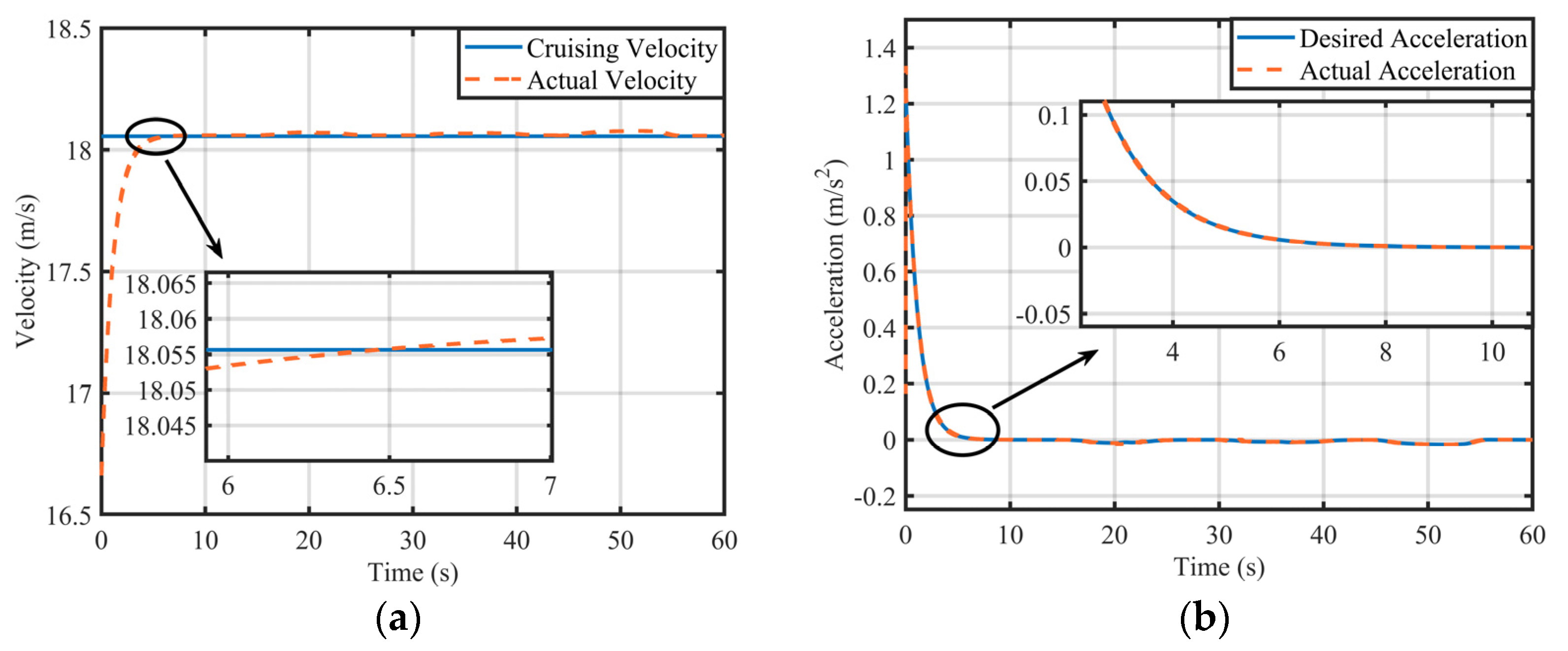
3.6.1. Constant Speed Cruise Driving Scenario

• Cruising Speed, 65 km/h (18.06 m/s);

In the constant speed cruise scenario, the simulation verification of the acceleration process is performed. Under the initial scenario, the host vehicle speed is set to 60 km/h (16.67 m/s), and the cruise speed is 18.06 m/s. The velocity and acceleration curves during the acceleration process are shown in Figure 9.

It can be seen from Figure 9 that the speed of the host vehicle is less than the cruising velocity at the beginning of the simulation. As the simulation time progresses, the speed of the host vehicle gradually approaches the cruising velocity (Figure 9a), and the acceleration also decreases and gradually approaches 0 (Figure 9b). When $t$ = 6.5 s, the host vehicle’s speed reaches the cruising speed and maintains a constant speed. It can be seen that there is a slight jitter in the velocity and acceleration curves, which is caused by the vehicle driving on a variable-curvature road. In general, in the acceleration process, the host vehicle has a better tracking effect on the cruising velocity.

2.

Cruising Speed, 45 km/h (12.5 m/s);

In the constant-speed-cruise scenario, the simulation verification of the deceleration process is performed. Under the initial scenario, the host vehicle’s speed is set to 16.67 m/s, and the cruising velocity is 12.5 m/s. The velocity and acceleration curves during the deceleration process are shown in Figure 10.

It can be seen from Figure 10 that the speed of the host vehicle is greater than the cruising velocity at the beginning of the simulation. As the simulation time progresses, the speed of the host vehicle gradually approaches the cruising velocity (Figure 10a), and the acceleration also increases and gradually approaches 0 (Figure 10b). When $t$ = 6.5 s, the host vehicle speed reaches the cruising velocity and maintains the constant speed. In the deceleration process, the host vehicle also has a better tracking effect on the cruising velocity.

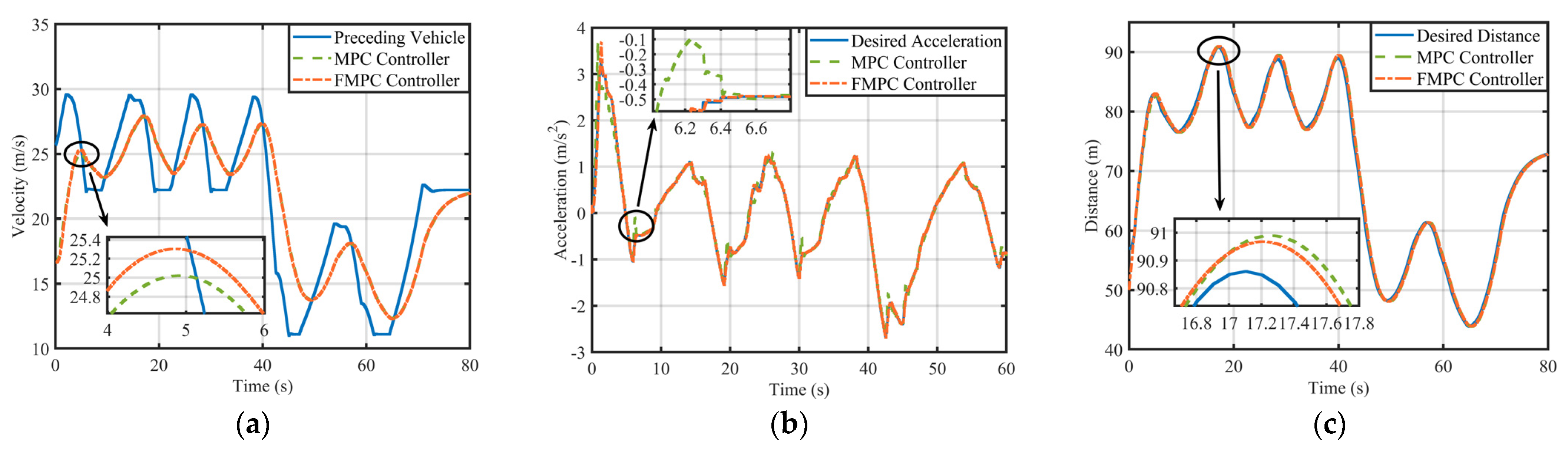
3.6.2. Distance Following Driving Scenario

The simulation sets the initial speed of the host vehicle and the preceding vehicle as 16.67 m/s and 80 km/h (22.22 m/s), respectively; the initial inter-distance is 50 m, and the speed of the preceding vehicle is changed via multiple acceleration and deceleration. The simulation results are shown in Figure 11.

It can be seen from Figure 11 that the control effect of FMPC designed in this paper is better than that of MPC with a constant weight. Although the host vehicle’s speed cannot fully track that of the preceding vehicle, its speed change is relatively subtle (Figure 11a). At the same time, the acceleration controlled via FMPC can track the ideal acceleration well. On the contrary, the acceleration controlled via MPC has several abnormal vibrations. For example, when t = 6.23 s, the acceleration error between FMPC and MPC is 0.468 m/s² (Figure 11b). Figure 11c shows that the distance curves of the two controllers can track the desired distance well, but the control effect of FMPC is better. For example, when t = 17.27 s, the distance curves reach the peak value, and the distance error between FMPC and MPC is 0.037 m. Therefore, the upper-level control algorithm based on the form of FMPC designed in this paper can meet the rapid response of the DSV under the curving cruise following scenario and achieve the control goal.

4. Lateral Stability Control of DSV Curving Cruise

In order to ensure the lateral stability of the DSV during the cruising process, this paper selects the yaw rate and the sideslip angle as the main parameters to measure stability [42]. By analyzing the motion state of DSV, the ideal front wheel’s steering angle is obtained via preview control and used as the input of the 2-DOF model used as the reference model, and the DSS controller is designed based on the SMC algorithm theory. The lateral stability of the DSV is realized by solving the differential torque.

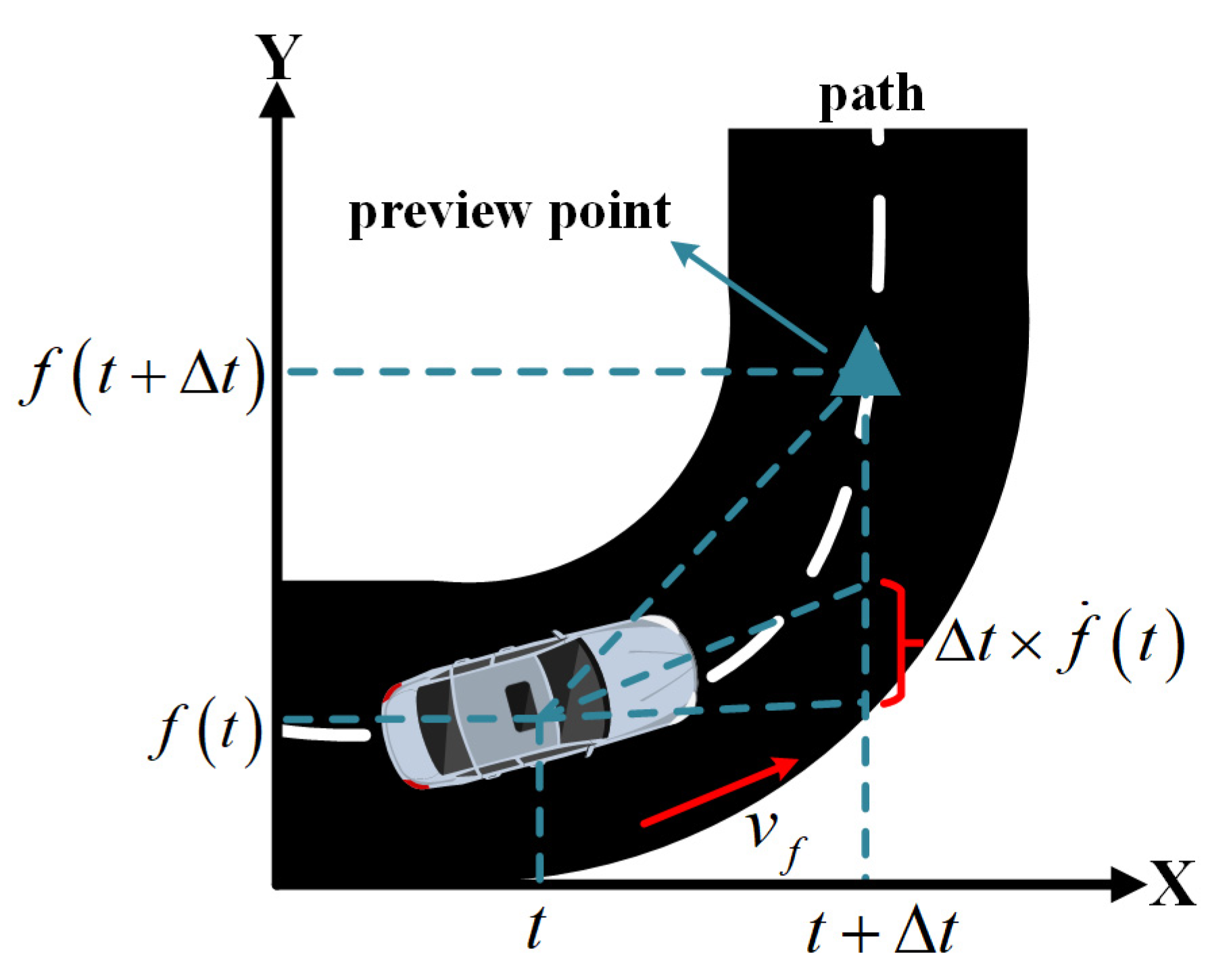
4.1. Preview Model Design

In this paper, preview control is used to obtain the road information and the preceding vehicle trajectory in advance [43,44], and the front wheel’s steering angle required for the next moment is judged according to the driving state of the vehicle and used as the input of the 2-DOF vehicle model. The yaw rate and sideslip angle can effectively compensate for the system delay problem. Figure 12 is a diagram of preview control model.

Figure 12 shows that in the process of preview, the ideal lateral distance and preview distance after the $∆t$ moment, are estimated using the deviation formed of road information and host vehicle heading.

$$f\left(t+∆t\right)=f\left(t\right)+∆t\times \dot{f}\left(t\right)+{∆t}^2\times \frac{1}{2}\ddot{f}\left(t\right)$$

(49)

$$d_{pre}=v_f\times ∆t$$

(50)

where $∆t$ is the forward-looking time, $f\left(t\right)$ is the lateral travel distance of the vehicle at time $t$, and $d_{pre}$ is the preview distance. According to the centripetal force acceleration, $a_y$, of the circular motion and parallel Equations (49) and (50), the yaw rate can be obtained as follows:

$$\omega =\frac{v_f}{R_c}=\frac{2v_f}{d_{pre}^2}\left[f\left(t+∆t\right)-f\left(t\right)-∆t\times \dot{f}\left(t\right)\right]$$

(51)

where $R_c$ is the curvature radius. At the same time, according to Equation (20) and the expression of the stability factor, $K$, the ideal front wheel’s steering angle input in the 2-DOF model can be calculated.

$${\delta }_d=\frac{2\left[f\left(t+∆t\right)-f\left(t\right)-∆t\times \dot{f}\left(t\right)\right]\times \left(1+K{v}_f^2\right)}{d_{pre}^2}$$

(52)

4.2. Lateral Stability Controller of DSV Based on SMC

The differential drive torque is obtained via the yaw rate and sideslip angle to control vehicle steering, thus ensuring the lateral stability of the DSV.

In order to make the deviation between the actual value and the ideal value zero, that is, $e_r={\lambda }_{\omega }\left(\omega -{\omega }_d\right)+{\lambda }_{\beta }\left(\beta -{\beta }_d\right)$, the sliding mode surface is defined as follows:

$$s=e_r+\lambda \left[{\int }_0^t{\lambda }_{\omega }\left(\omega -{\omega }_d\right)dt+{\int }_0^t{\lambda }_{\beta }\left(\beta -{\beta }_d\right)dt\right]$$

(53)

where ${\lambda }_{\omega }$ and ${\lambda }_{\beta }$ are the relative weight of $\omega$ deviation and the relative weight of $\beta$ deviation, respectively.

The following is the SMC rate selection exponential reaching law [45]:

$$\dot{s}=-\epsilon \times sgn\left(s\right)-ks$$

(54)

where $\epsilon$ and $k$ are the exponential approach rate parameters based on $\omega$ and $\beta$. In order to suppress the chattering of the system, the value of $k$ is increased and the value of $\epsilon$ is reduced in the design.

According to Equations (9), (53) and (54), the required differential moment for the DSV can be obtained as follows:

$$∆T=\frac{\dot{s}-\lambda e+{\lambda }_{\omega }{\dot{\omega }}_d+{\lambda }_{\beta }{\dot{\beta }}_d-{\lambda }_{\omega }{f}_1-{\lambda }_{\beta }{f}_2}{{\lambda }_{\omega }{g}_1}$$

(55)

where $f_1$, $f_2$, and $g_1$ are

$$\left\{\begin{array}{c}{f}_1=\frac{b{k}_r-a{k}_f}{I_z}\beta -\frac{a^2{k}_f+b^2{k}_r}{I_z{v}_x}\omega +\frac{a{k}_f}{I_z}\delta \\ f_2=-\frac{k_f+k_r}{m{v}_x}\beta +\left(\frac{b{k}_r-a{k}_f}{m{v}_x^2}-1\right)\omega +\frac{k_f}{m{v}_x}\delta \\ g_1=\frac{l_s}{I_{z}R}\end{array}\right.$$

(56)

5. Analysis of Simulation Results

This paper designs two simulation scenarios, one in which the preceding vehicle runs at a constant speed and another in which it runs at a variable speed, respectively. The S-Turn driving condition is used for simulation verification. It is also compared with the current common combined MPC and DYC control strategy. The longitudinal speed and inter-vehicle distance tracking of both control strategies are very good, so this paper will focus on analyzing the comparison of lateral stability.

5.1. The Simulation of the Preceding Vehicle Driving at a Constant Speed

The initial driving speed of the host vehicle is 16.67 m/s, the initial distance is 50 m, and the preceding vehicle runs at a constant speed of 22.22 m/s, while the simulation time is 80 s. The simulation results are shown in Figure 13.

Figure 13 shows the simulation results of the driving state of the host vehicle when the preceding vehicle is driving at a uniform speed on a variable-curvature curve. It can be seen from Figure 13a–c that the speed of the host vehicle is adjusted to a speed range similar to that of the preceding vehicle at about $t$ = 22.55 s, and the speed changes gently, which is in accordance with the driver’s actual car-following conditions (Figure 13a). At the same time, the acceleration is controlled within the range of −0.112~1.167 m/s², which is in accordance with the comfort constraint condition (Figure 13b). After the speed is stable, the speed error is controlled within 0.018 m/s, and the error between the actual distance and the desired distance is controlled within 0.105 m (Figure 13c), which ensures longitudinal safety during the curving car-following process.

From Figure 13d, it can be seen that the trajectory of the host vehicle with two types of control strategies or without the stability controller can better track the desired trajectory. Comparing the control effect of MPC with that of DYC, the trajectory controlled via the proposed strategy of control in this paper is closer to the desired trajectory. The error of the two control strategies is 0.07 m when $t$ = 29.86 s. At the same time, Figure 13e,f shows that the tracking effect of the sideslip angle and yaw rate controlled via the proposed control strategy is better. The errors of the two control strategies are 4 × 10⁻⁵ rad and 9 × 10⁻⁴ rad/s when $t$ = 18.65 s, respectively. Therefore, the DSV controlled by proposed control in this paper can maintain vehicle distance control accuracy while maintaining better lateral stability than that of MPC with DYC, and meet the needs of curving ACC system cruising.

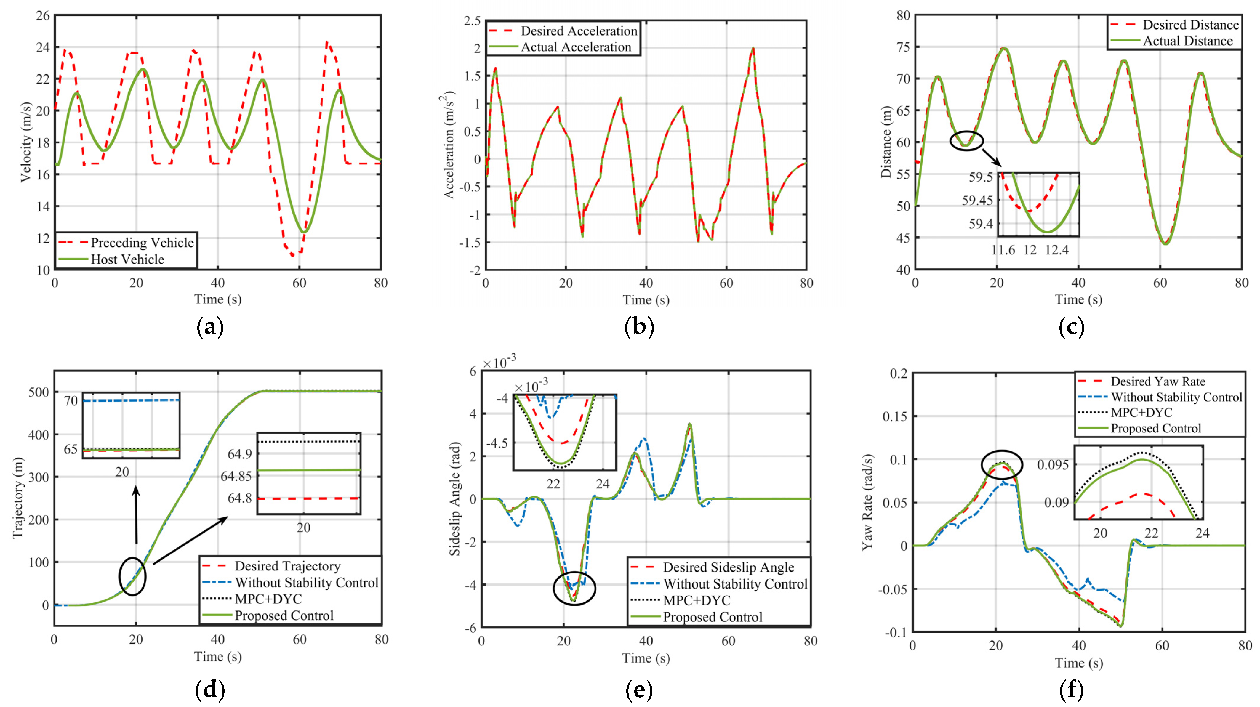
5.2. The Simulation of the Preceding Vehicle Driving at a Variable Speed

The initial driving speed of the host vehicle is 16.67 m/s, the initial distance is 50 m, and the preceding vehicle runs at a variable speed, while the simulation time is 80 s. The simulation results are shown in Figure 14.

Figure 14 is the simulation results of the driving state of the host vehicle when the preceding vehicle is driving at a variable speed on a variable curvature curve. It can be seen from Figure 14a–c that at the beginning of the simulation, the speed of the host vehicle is lower than the speed of the preceding vehicle, and the host vehicle is gradually close to the preceding vehicle through the drive. The relative distance between the two vehicles becomes gradually close to the desired distance, and the speed is adjusted to a speed range close to the preceding vehicle at $t$ = 5.37 s. As shown in Figure 14a,c, it can be seen that the maximum error of the speed of the two vehicles is about 3.18 m/s, the maximum error of the distance is 0.6 m, and the maximum error occurs when the speed of the preceding vehicle changes abruptly. Figure 14b shows that the acceleration of the host vehicle is controlled in the range of −1.5~2 m/s², which satisfies the constraint conditions. Therefore, the FMPC control strategy designed in this paper can make the host vehicle have a good longitudinal tracking effect.

From Figure 14d, it can be seen that the trajectory of the host vehicle with two types of controllers can better track the desired trajectory. Compared with the control effect of the MPC with DYC, the trajectory controlled via the proposed control strategy in this paper is closer to the desired trajectory. The error of the two control strategies is 0.065 m when $t$ = 20 s. At the same time, Figure 14e,f shows that the tracking effect of the sideslip angle and yaw rate controlled via the proposed control strategy is better than MPC with DYC. When $t$ = 22.31 s, the errors of the two control strategies are 5 × 10⁻⁵ rad and 9 × 10⁻⁴ rad/s, respectively. Therefore, the simulation results verify the effectiveness of the control strategy proposed in this paper. Meanwhile, compared with the control effect of MPC with DYC, the control strategy proposed in this paper has a better effect.

6. Conclusions

In this paper, the control strategy for the multi-objective optimization of curving ACC is designed for the DSV, which includes longitudinal speed and inter-distance control as well as lateral stability control. The fuzzy control rules are designed to change the weight matrix of the performance indicators in real time. The fuzzy rules take the improvement of economy as the main goal, while coordinating the relationship between other performance indicators. The lateral stability control strategy is designed based on the preview and SMC algorithms to ensure the vehicle’s longitudinal following performance as much as possible on curved roads.

The control strategy proposed in this paper ensures that the longitudinal inter-vehicle distance, speed, and acceleration are controlled within the driver’s acceptance ranges. Compared to MPC with a constant weight matrix, economy is improved by 21.76% while ensuring safe following driving. The lateral stability of the DSV is ensured by controlling the differential torque of the front wheels. The effectiveness and advantages of the control strategy proposed in this paper are verified by comparing it with the control effect of MPC with DYC. The control strategy proposed in this paper extends the usage scenario of the ACC system so that the DSV can realize multi-objective coordinated control on curved roads. It is beneficial to reducing the occurrence of vehicle collisions and improving energy consumption.

7. Future Work and Prospects

This paper combines the ACC system with the SBW technology. In the process of vehicle following, the stabilization of the vehicle on curve roads is achieved by controlling the front wheel’s differential torque in the electric vehicle driven by in-wheel motors. The common S-turn road condition in reality is selected for simulation verification, so that the simulation results have practical significance.

The present paper has the following limitations. Firstly, bad weather conditions are not considered, such as heavy rain and snowstorms; these can have an effect on the longitudinal and lateral control effects of ACC vehicles. In future work, we will analyze the possible effects of bad weather on vehicles and design reasonable control strategies. Secondly, there are some differences between the curved driving environment built in the simulation software and the real driving environment. In future work, we will combine the real curved road driving environment with the simulated one to carry out algorithm optimization and control strategy optimization. Finally, only the stability of the host vehicle when following the preceding vehicle is considered in this paper. However, in the real driving environment, traffic density needs to be considered. In future work, we will research vehicle platoon stability control to further improve road utilization.

References

1. Li, Z.; Deng, Y.; Sun, S. Adaptive Cruise Predictive Control Based on Variable Compass Operator Pigeon-Inspired Optimization. Electronics 2022, 11, 1377. [Google Scholar] [CrossRef]
2. Bekiaris-Liberis, N.; Roncoli, C.; Papageorgiou, M. Predictor-Based Adaptive Cruise Control Design with Integral Action. IFAC-PapersOnLine 2018, 51, 86–91. [Google Scholar] [CrossRef]
3. Xiao, G.; Zhang, H.; Sun, N.; Zhang, Y. Cooperative Link Scheduling for RSU-Assisted Dissemination of Basic Safety Messages. Wirel. Netw. 2021, 27, 1335–1351. [Google Scholar] [CrossRef]
4. Yao, J.; Ge, Z. Path-Tracking Control Strategy of Unmanned Vehicle Based on DDPG Algorithm. Sensors 2022, 22, 7881. [Google Scholar] [CrossRef] [PubMed]
5. Lian, J. The Intelligent Vehicle Control System Based on the Fuzzy Neural Network Technology. Adv. Mater. Res. 2012, 487, 830–835. [Google Scholar] [CrossRef]
6. Gao, H.; Zhang, X.; Liu, Y.; Li, D. Cloud Model Approach for Lateral Control of Intelligent Vehicle Systems. Sci. Program. 2016, 2016, 6842891. [Google Scholar] [CrossRef]
7. Abbasimoshaei, A.; Chinnakkonda Ravi, A.K.; Kern, T.A. Development of a New Control System for a Rehabilitation Robot Using Electrical Impedance Tomography and Artificial Intelligence. Biomimetics 2023, 8, 420. [Google Scholar] [CrossRef] [PubMed]
8. Shang, M.; Rosenblad, B.; Stern, R. A Novel Asymmetric Car Following Model for Driver-Assist Enabled Vehicle Dynamics. IEEE Trans. Intell. Transp. Syst. 2022, 23, 15696–15706. [Google Scholar] [CrossRef]
9. Guo, Y.; Sun, Q.; Fu, R.; Wang, C. Improved Car-Following Strategy Based on Merging Behavior Prediction of Adjacent Vehicle from Naturalistic Driving Data. IEEE Access 2019, 7, 44258–44268. [Google Scholar] [CrossRef]
10. Yen, Y.; Chou, J.; Shih, C.; Chen, C.; Tsung, P. Proactive Car-Following Using Deep-Reinforcement Learning. In Proceedings of the 23rd IEEE International Conference on Intelligent Transportation Systems, Rhodes, Greece, 20–23 September 2020. [Google Scholar]
11. Moon, S.; Yi, K. Human Driving Data-Based Design of a Vehicle Adaptive Cruise Control Algorithm. Veh. Syst. Dyn. 2008, 46, 661–690. [Google Scholar] [CrossRef]
12. Moon, S.; Yi, K.; Kang, H.; Yoon, P. Adaptive Cruise Control with Collision Avoidance in Multi-Vehicle Traffic Situations. SAE Tech. Pap. 2009, 2, 653–660. [Google Scholar] [CrossRef]
13. Mohtavipour, S.M.; Mollajafari, M. An Analytically Derived Reference Signal to Guarantee Safety and Comfort in Adaptive Cruise Control Systems. J. Intell. Transp. Syst. 2021, 25, 1–20. [Google Scholar] [CrossRef]
14. Das, L.; Won, M. SAINT-ACC: Safety-Aware Intelligent Adaptive Cruise Control for Autonomous Vehicles Using Deep Reinforcement Learning. Proc. Mach. Learn. Res. 2021, 139, 2445–2455. [Google Scholar]
15. Li, S.E.; Jia, Z.; Li, K.; Cheng, B. Fast Online Computation of a Model Predictive Controller and Its Application to Fuel Economy-Oriented Adaptive Cruise Control. IEEE Trans. Intell. Transp. Syst. 2015, 16, 1199–1209. [Google Scholar] [CrossRef]
16. Lin, Y.C.; Nguyen, H.L.T.; Balas, V.E.; Lin, T.C.; Kuo, I.C. Adaptive Prediction-Based Control for an Ecological Cruise Control System on Curved and Hilly Roads. J. Intell. Fuzzy Syst. 2020, 38, 6129–6144. [Google Scholar] [CrossRef]
17. Tian, J.; Zeng, Q.; Wang, P.; Wang, X. Active Steering Control Based on Preview Theory for Articulated Heavy Vehicles. PLoS ONE 2021, 16, e0252098. [Google Scholar] [CrossRef]
18. Guo, J.H.; Luo, Y.G.; Li, K.Q. Adaptive Fuzzy Sliding Mode Control for Coordinated Longitudinal and Lateral Motions of Multiple Autonomous Vehicles in a Platoon. Sci. China Technol. Sci. 2017, 60, 576–586. [Google Scholar] [CrossRef]
19. Zhang, D.; Li, K.; Wang, J. A Curving ACC System with Coordination Control of Longitudinal Car-Following and Lateral Stability. Veh. Syst. Dyn. 2012, 50, 1085–1102. [Google Scholar]
20. Li, H.; Li, J.; Su, Z.; Wang, X.; Luo, J. Research on Active Obstacle Avoidance Control Strategy for Intelligent Vehicle Based on Active Safety Collaborative Control. IEEE Access 2020, 8, 183736–183748. [Google Scholar] [CrossRef]
21. Idriz, A.F.; Rachman, A.S.A.; Baldi, S. Integration of Auto-Steering with Adaptive Cruise Control for Improved Cornering Behaviour. IET Intell. Transp. Syst. 2017, 11, 667–675. [Google Scholar] [CrossRef]
22. Gao, F.; Zhao, F.; Zhang, Y. Research on Path Tracking and Yaw Stability Coordination Control Strategy for Four-Wheel Independent Drive Electric Trucks. Processes 2023, 11, 2473. [Google Scholar] [CrossRef]
23. Tian, J.; Yang, M. Hierarchical Control of Differential Steering for Four-in-Wheel-Motor Electric Vehicle. PLoS ONE 2023, 18, e0285485. [Google Scholar] [CrossRef]
24. Tian, J.; Yang, M. Research on Trajectory Tracking and Body Attitude Control of Autonomous Ground Vehicle Based on Differential Steering. PLoS ONE 2023, 18, e0273255. [Google Scholar] [CrossRef]
25. Chen, T.; Cai, Y.; Chen, L.; Xu, X.; Sun, X. Trajectory Tracking Control of Steer-by-Wire Autonomous Ground Vehicle Considering the Complete Failure of Vehicle Steering Motor. Simul. Model. Pract. Theory 2021, 109, 102235. [Google Scholar] [CrossRef]
26. Tian, H.; Zhu, W.; Wang, S. Adaptive Electronic Differential Control of Vehicle by Torque Balance. Mob. Netw. Appl. 2020, 25, 1604–1610. [Google Scholar] [CrossRef]
27. Li, C.; Xie, Y.F.; Wang, G.; Liu, S.Q.; Kuang, B.; Jing, H. Experimental Study of Electric Vehicle Yaw Rate Tracking Control Based on Differential Steering. J. Adv. Transp. 2021, 2021, 6668091. [Google Scholar] [CrossRef]
28. Du, P.; Ma, Z.; Chen, H.; Xu, D.; Wang, Y.; Jiang, Y.; Lian, X. Speed-Adaptive Motion Control Algorithm for Differential Steering Vehicle. Proc. Inst. Mech. Eng. Part D J. Automob. Eng. 2021, 235, 672–685. [Google Scholar] [CrossRef]
29. Zheng, C.; Xu, D.; Cao, J.; Li, W. Design of Lightweight Electric Forestry Monorail Vehicle. J. For. Eng. 2021, 6, 140–146. [Google Scholar] [CrossRef]
30. Zhang, S.; Liu, C.; Wu, X.; Chen, Z.; Huang, X.; Lin, J. Design of Automatic Cut-off Machine with Selected Length to Bamboo and Analysis of Corresponding Movement. J. For. Eng. 2021, 6, 143–146. [Google Scholar] [CrossRef]
31. Li, H.; Wang, L.; Wang, F.; Li, Z. Research on Multi-Objective Optimization of Support Parameters of High-Speed Railway Tunnel. J. For. Eng. 2021, 6, 169–175. [Google Scholar] [CrossRef]
32. Peng, F.; Wang, Y.; Xuan, H.; Nguyen, T.V.T. Efficient Road Traffic Anti-Collision Warning System Based on Fuzzy Nonlinear Programming. Int. J. Syst. Assur. Eng. Manag. 2022, 13, 456–461. [Google Scholar] [CrossRef]
33. Nguyen, T.V.T.; Huynh, N.T.; Vu, N.C.; Kieu, V.N.D.; Huang, S.C. Optimizing Compliant Gripper Mechanism Design by Employing an Effective Bi-Algorithm: Fuzzy Logic and ANFIS. Microsyst. Technol. 2021, 27, 3389–3412. [Google Scholar] [CrossRef]
34. Vu, T.M.; Moezzi, R.; Cyrus, J.; Hlava, J. Model Predictive Control for Autonomous Driving Vehicles. Electronics 2021, 10, 2593. [Google Scholar] [CrossRef]
35. Guo, L.; Ge, P.; Sun, D.; Qiao, Y. Adaptive Cruise Control Based on Model Predictive Control with Constraints Softening. Appl. Sci. 2020, 10, 1635. [Google Scholar] [CrossRef]
36. Shakouri, P.; Ordys, A. Nonlinear Model Predictive Control Approach in Design of Adaptive Cruise Control with Automated Switching to Cruise Control. Control Eng. Pract. 2014, 26, 160–177. [Google Scholar] [CrossRef]
37. Ali, Z.; Popov, A.A.; Charles, G. Model Predictive Control with Constraints for a Nonlinear Adaptive Cruise Control Vehicle Model in Transition Manoeuvres. Veh. Syst. Dyn. 2013, 51, 943–963. [Google Scholar] [CrossRef]
38. Ye, H.; Jiang, H.; Ma, S.; Tang, B.; Wahab, L. Linear Model Predictive Control of Automatic Parking Path Tracking with Soft Constraints. Int. J. Adv. Robot. Syst. 2019, 16, 1729881419852201. [Google Scholar] [CrossRef]
39. Gao, H.; Kan, Z.; Li, K. Robust Lateral Trajectory Following Control of Unmanned Vehicle Based on Model Predictive Control. IEEE/ASME Trans. Mechatron. 2022, 27, 1278–1287. [Google Scholar] [CrossRef]
40. Cai, J.; Jiang, H.; Chen, L.; Liu, J.; Cai, Y.; Wang, J. Implementation and Development of a Trajectory Tracking Control System for Intelligent Vehicle. J. Intell. Robot. Syst. 2019, 94, 251–264. [Google Scholar] [CrossRef]
41. Deng, X.; Sun, H.; Lu, Z.; Cheng, Z.; An, Y.; Chen, H. Research on Dynamic Analysis and Experimental Study of the Distributed Drive Electric Tractor. Agriculture 2023, 13, 40. [Google Scholar] [CrossRef]
42. Gao, F.; Zhao, F.; Zhang, Y. Research on Yaw Stability Control Strategy for Distributed Drive Electric Trucks. Sensors 2023, 23, 7222. [Google Scholar] [CrossRef] [PubMed]
43. Zhang, S.; Zhao, X.; Zhu, G.; Shi, P.; Hao, Y.; Kong, L. Adaptive Trajectory Tracking Control Strategy of Intelligent Vehicle. Int. J. Distrib. Sens. Netw. 2020, 16, 1550147720916988. [Google Scholar] [CrossRef]
44. Yim, S. Design of Preview Controllers for Active Roll Stabilization. J. Mech. Sci. Technol. 2018, 32, 1805–1813. [Google Scholar] [CrossRef]
45. Moshaii, A.A.; Moghaddam, M.M.; Niestanak, V.D. Analytical Model of Hand Phalanges Desired Trajectory for Rehabilitation and Design a Sliding Mode Controller Based on This Model. Modares Mech. Eng. 2020, 20, 129–137. [Google Scholar]
Figure 1. Diagram of 3-DOF vehicle dynamics model.
Electronics 12 04178 g001
Figure 2. Differential steering system schematic diagram.
Electronics 12 04178 g002
Figure 3. Linear 2-DOF vehicle model.
Electronics 12 04178 g003
Figure 4. The structure diagram of curving ACC control strategy of the DSV.
Electronics 12 04178 g004
Figure 5. The kinematic relationship between two vehicles.
Electronics 12 04178 g005
Figure 6. Cost function weight adjustment system based on fuzzy logic.
Electronics 12 04178 g006
Figure 7. Fuzzy logic control rules of parameter weights: (a) weight coefficient of relative distance; (b) weight coefficient of relative velocity; (c) weight coefficient of host vehicle acceleration.
Electronics 12 04178 g007
Figure 8. The switching logic flow chart of cruise mode and following mode.
Electronics 12 04178 g008
Figure 9. Simulation results of acceleration process under constant speed cruise scenario: (a) velocity change curves; (b) acceleration change curves.
Electronics 12 04178 g009
Figure 10. Simulation results of deceleration process under constant speed cruise scenario: (a) velocity change curves; (b) acceleration change curves.
Electronics 12 04178 g010
Figure 11. Simulation results under the following scenarios: (a) velocity change curve; (b) acceleration change curve; (c) distance change curve.
Electronics 12 04178 g011
Figure 12. The diagram of the preview control model.
Electronics 12 04178 g012
Figure 13. Simulation results under the scenario which the preceding vehicle driving at a constant speed: (a) velocity change curves; (b) acceleration change curves; (c) distance change curves; (d) trajectory change curves; (e) sideslip angle change curves; (f) yaw rate change curves.
Electronics 12 04178 g013
Figure 14. Simulation results under the scenario in which the preceding vehicle is driving at a variable speed: (a) velocity change curves; (b) acceleration change curves; (c) distance change curves; (d) trajectory change curves; (e) sideslip angle change curves; (f) yaw rate change curves.
Electronics 12 04178 g014