
Optimization of Multi-Phase Motor Drive System Design through Thermal Analysis and Experimental Validation of Heat Dissipation


Abstract
:1. Introduction
- The design attempted to overcome the limitations with significant modularity to accommodate not only six-phase and dual three-phase but also various multi-phase motors in the future.
- To make it easier to expand the capacity of each unit inverter, thermal analysis was performed in the form of a unit and an overall configuration to prevent thermal runaway of individual unit inverters, and various variables were considered in the verification stage.
- By comparing the simulation results with the actual experimental verification, the completeness of the simulation was verified in the design for modular inverters for multi-phase motors.
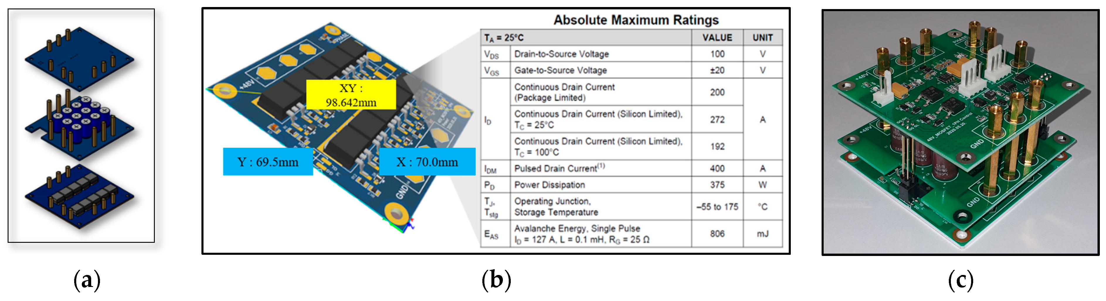
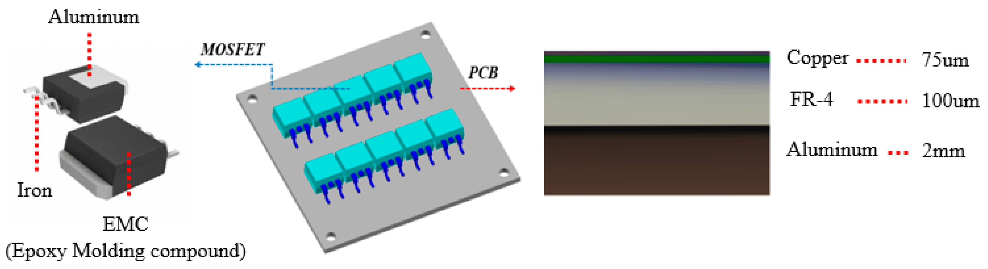
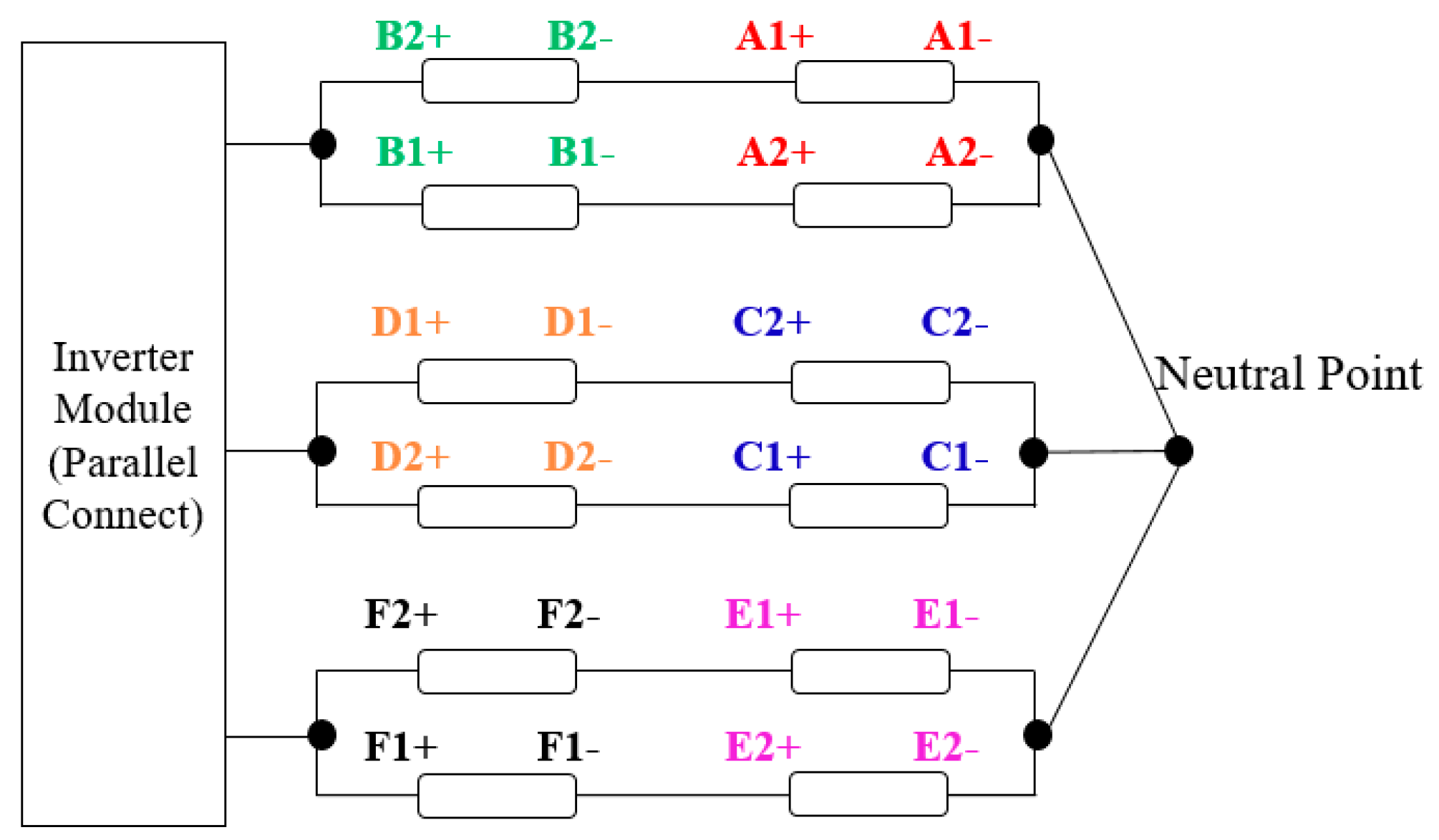
2. Inverter Design and Structure for Multi-Phase Motor Drive System
3. Simulations for Multi-Phase Inverter Design
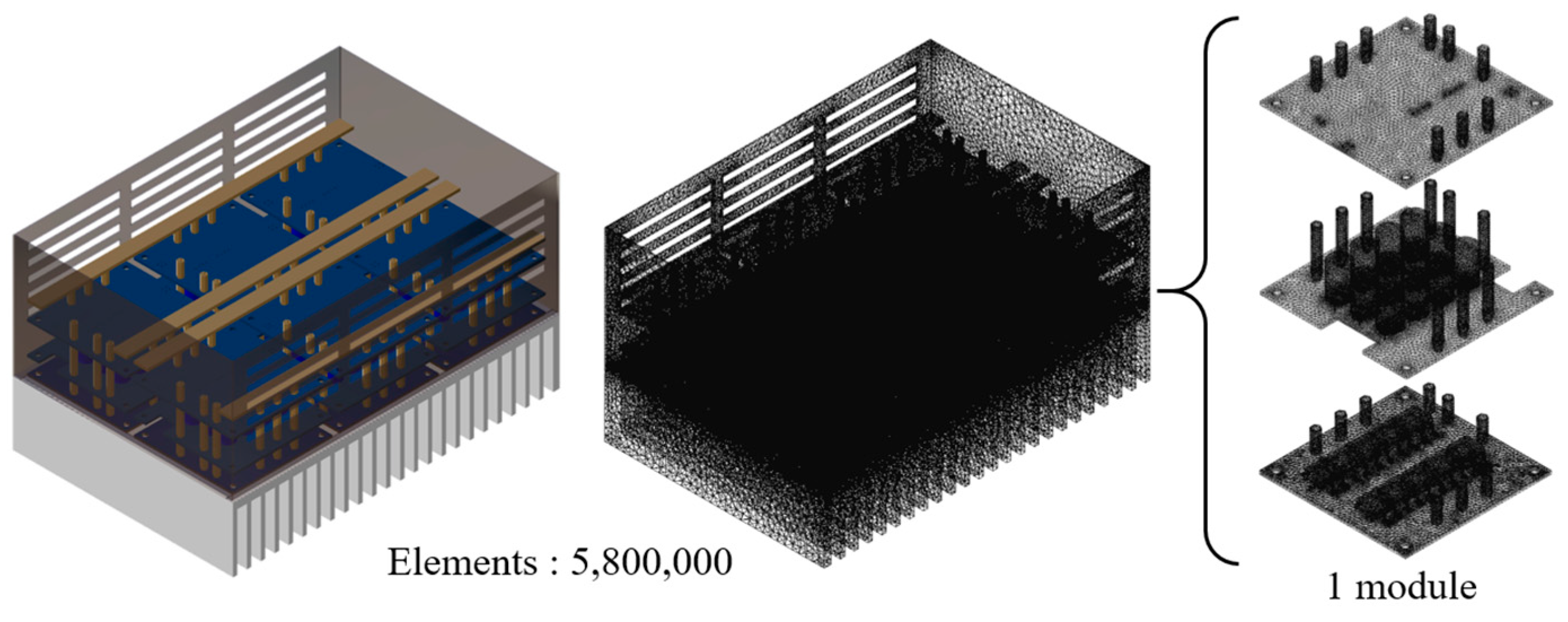
3.1. Power Analysis for Inverter Module and CFD Analysis
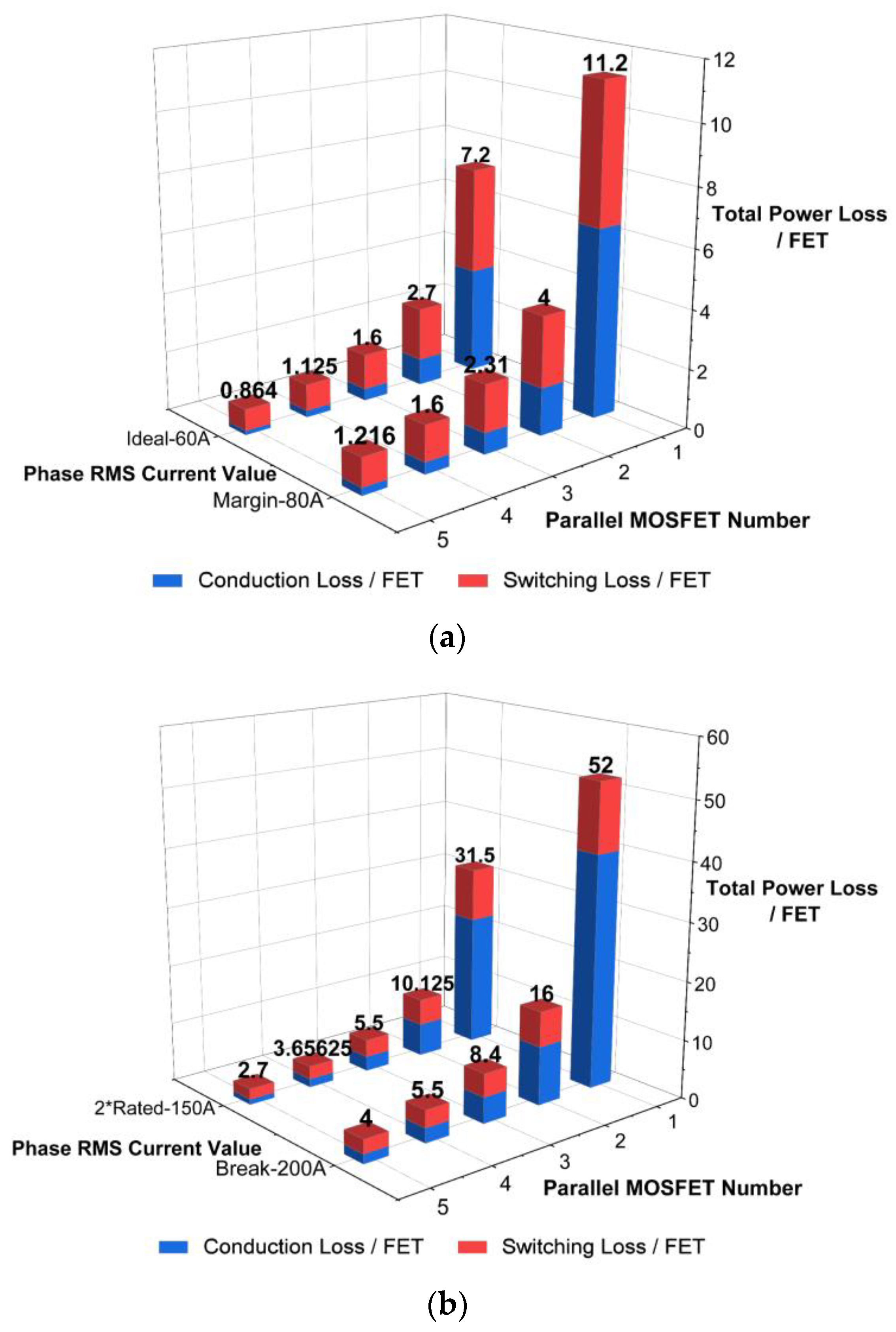
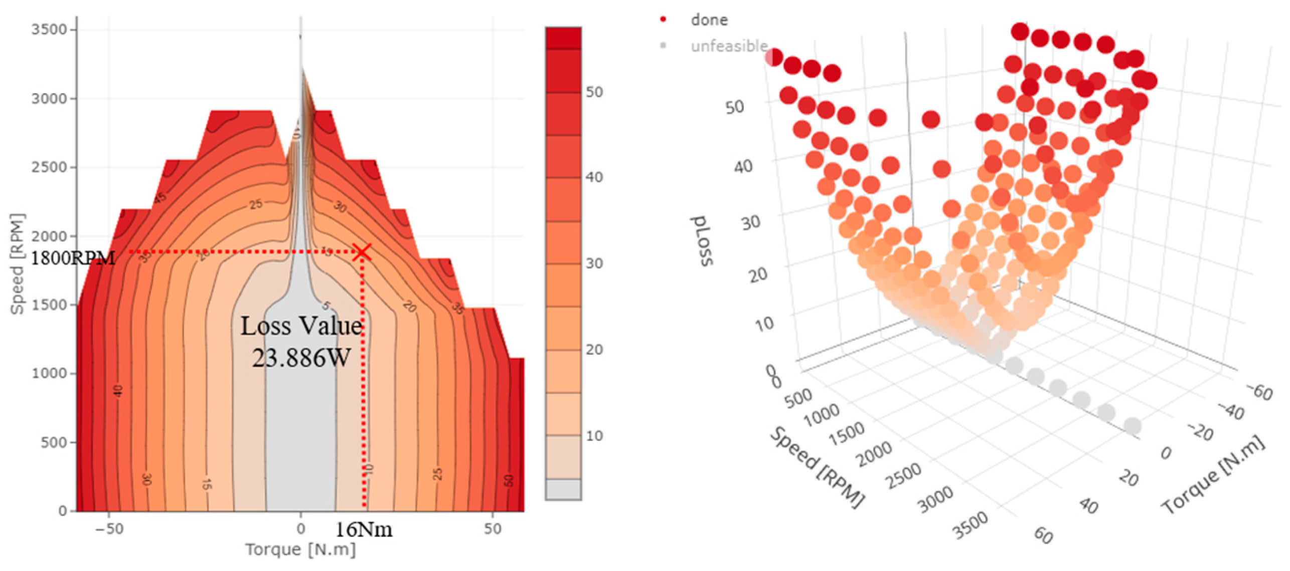
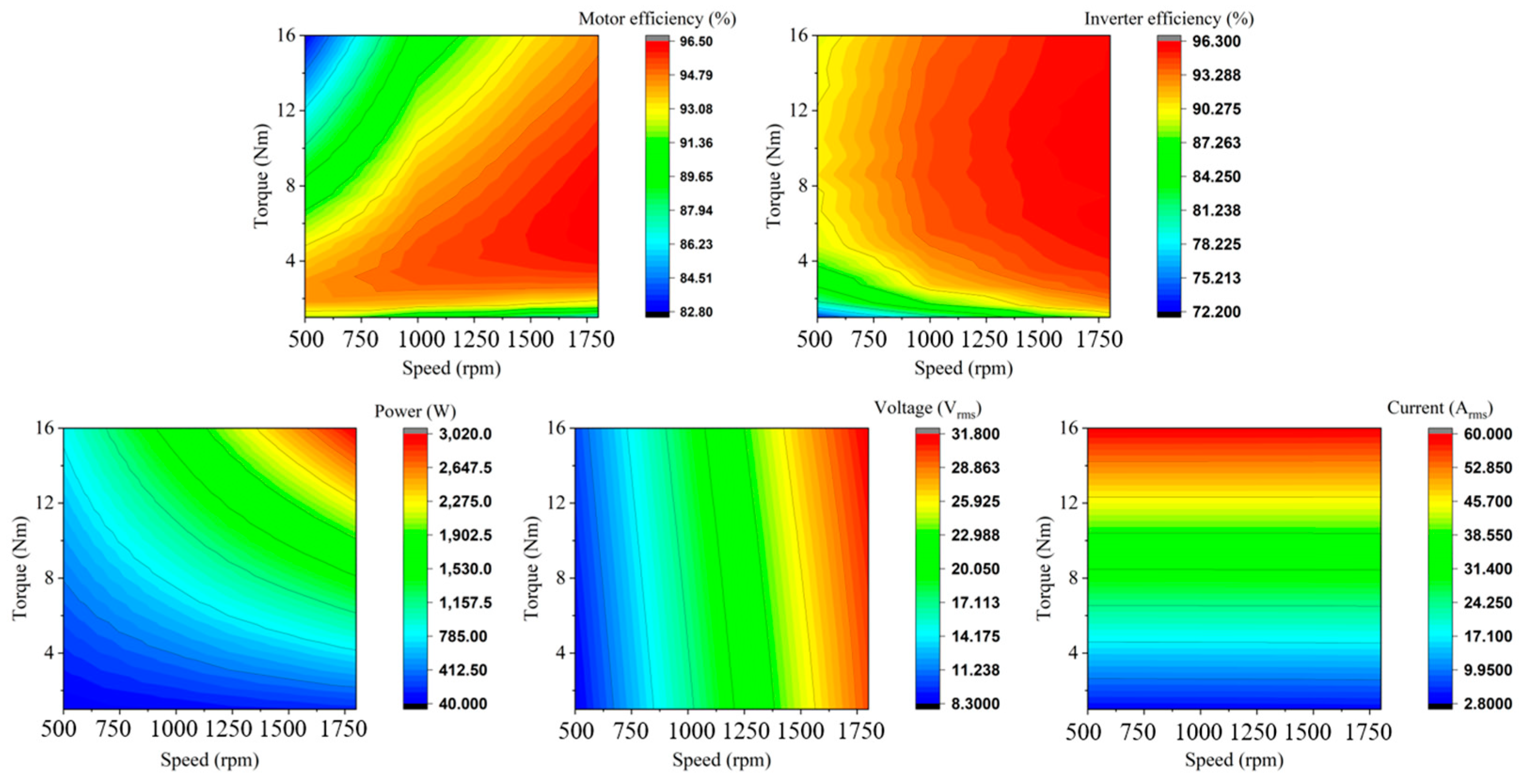
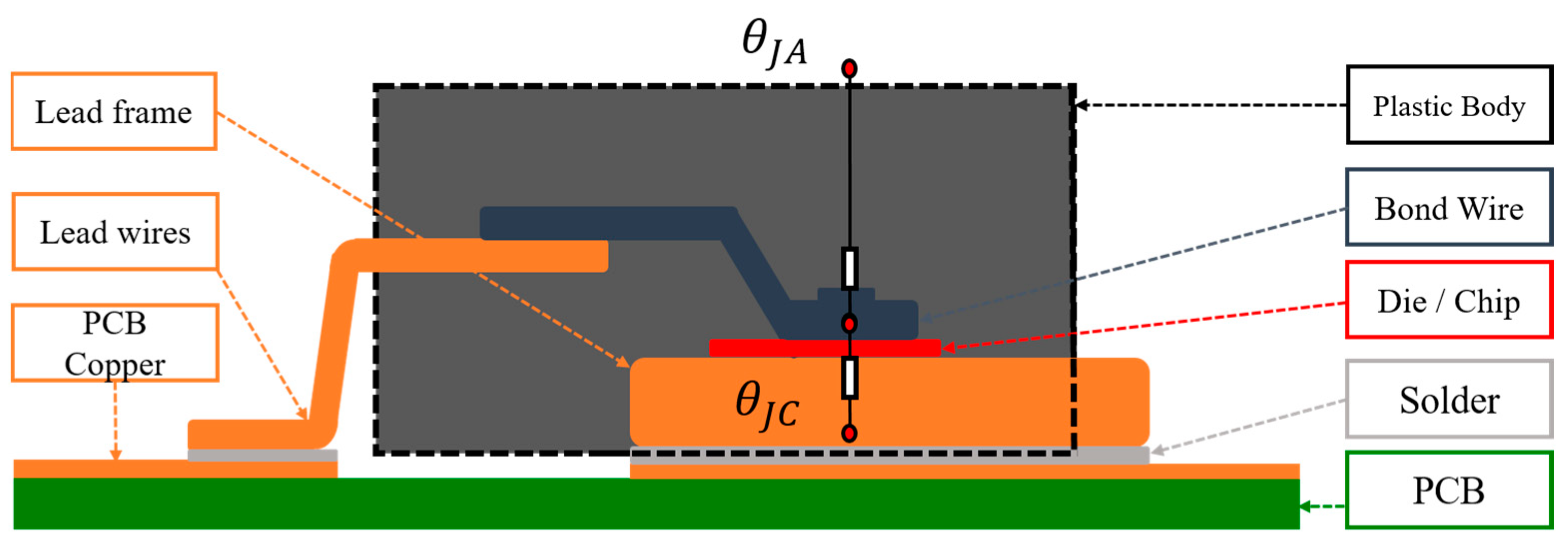
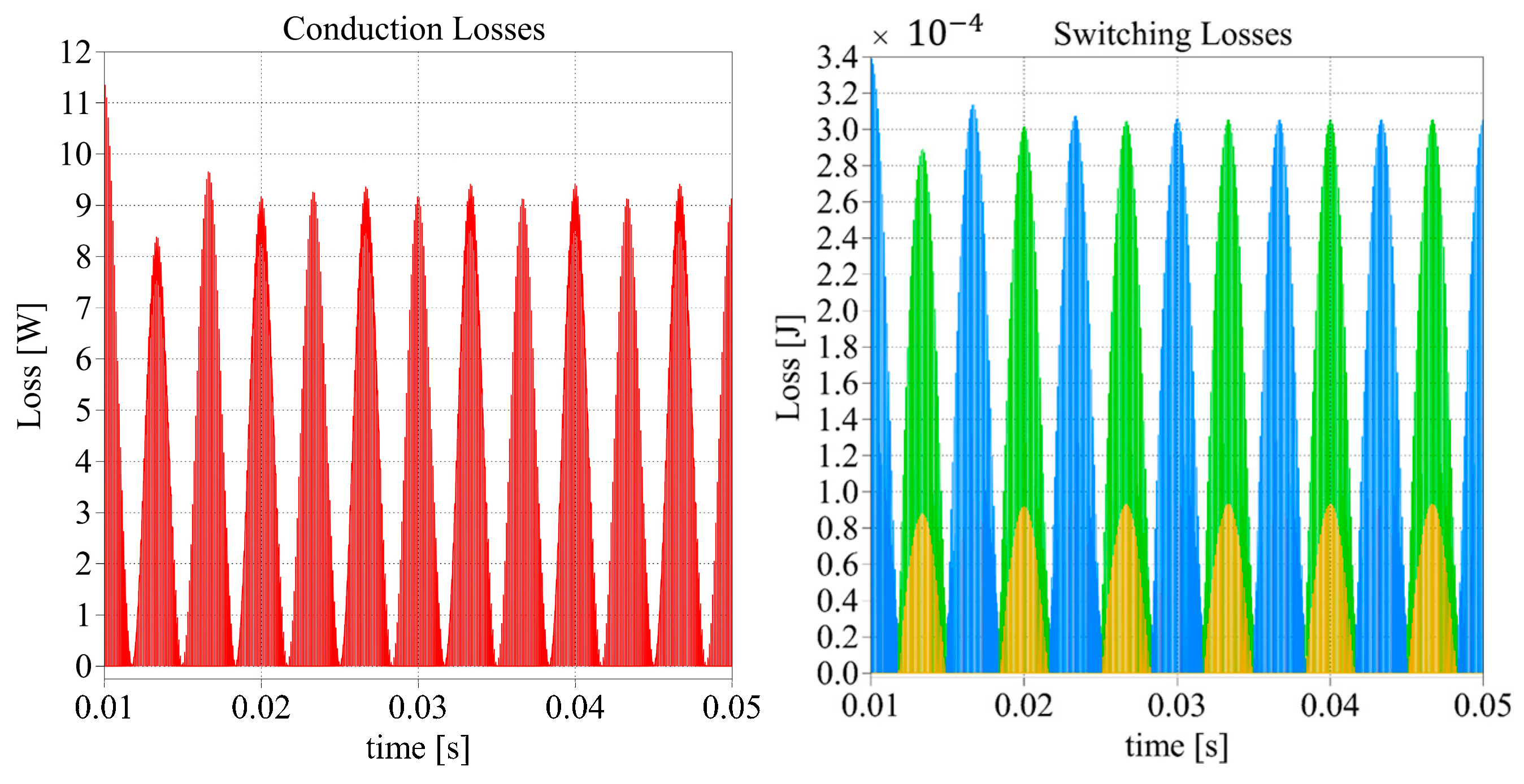
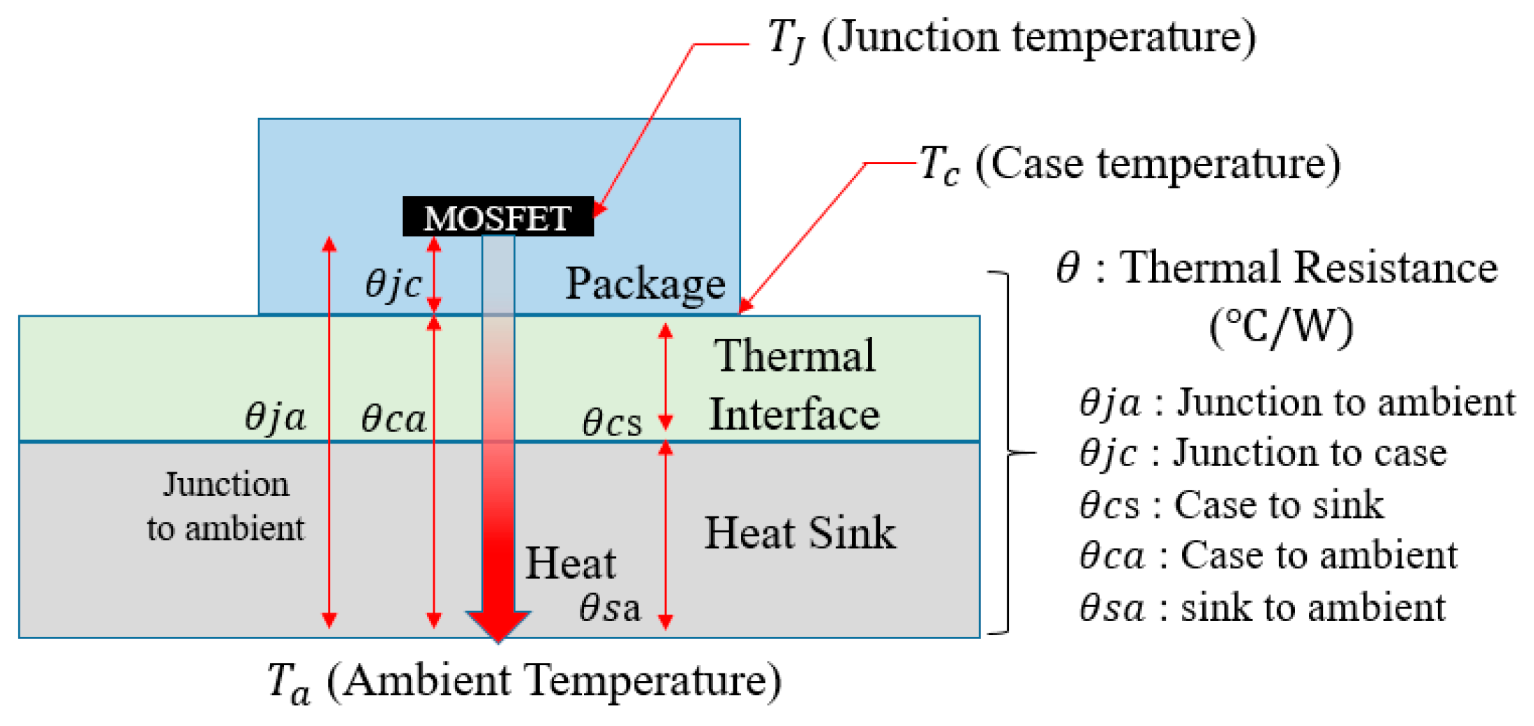
3.1.1. Power Electronics Analysis
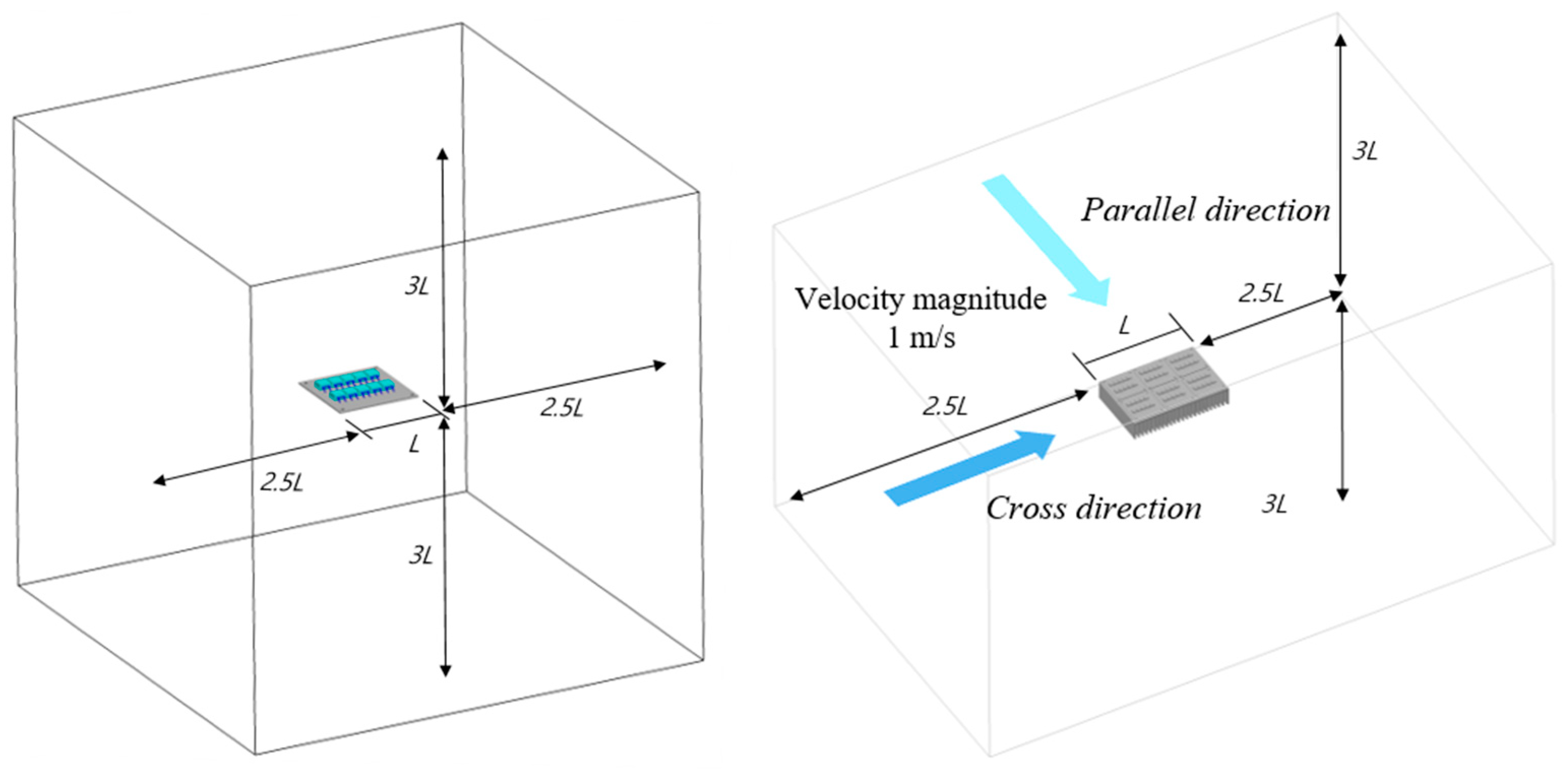
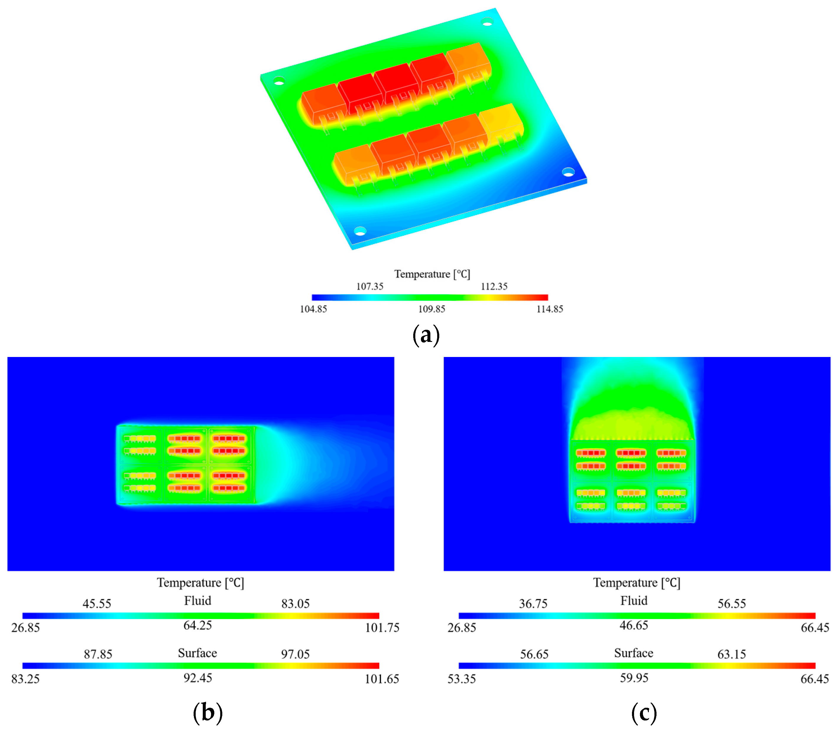
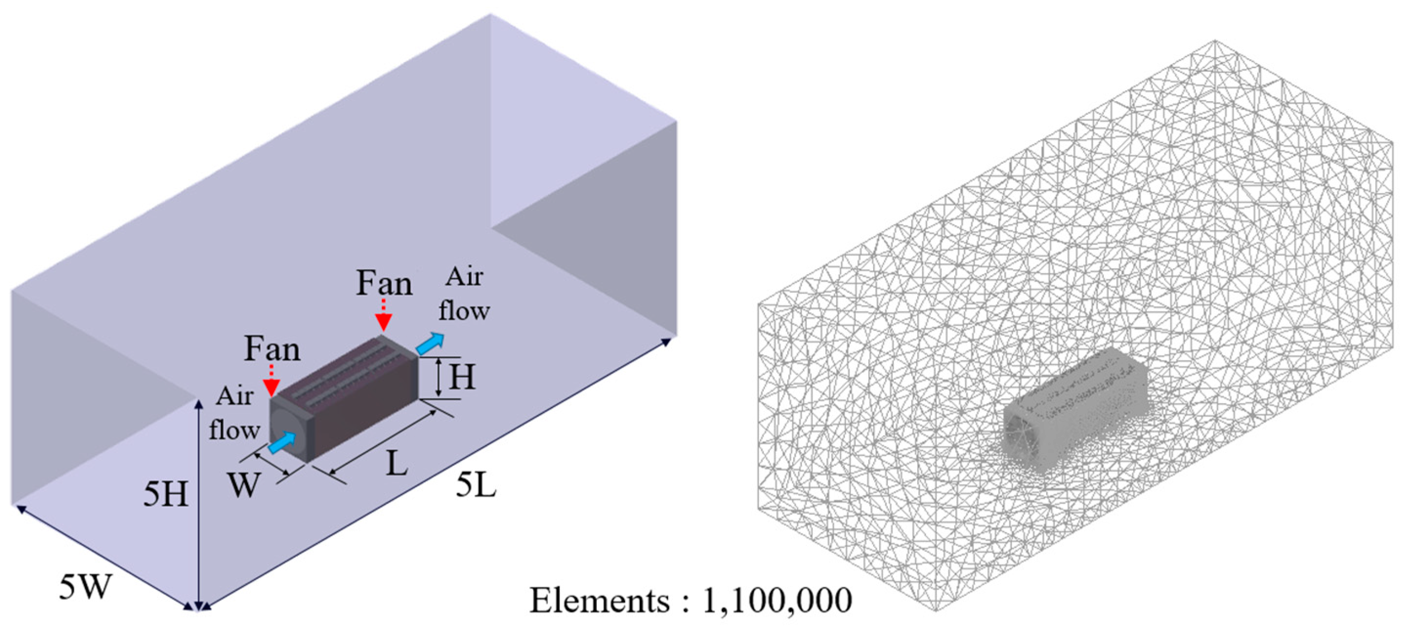
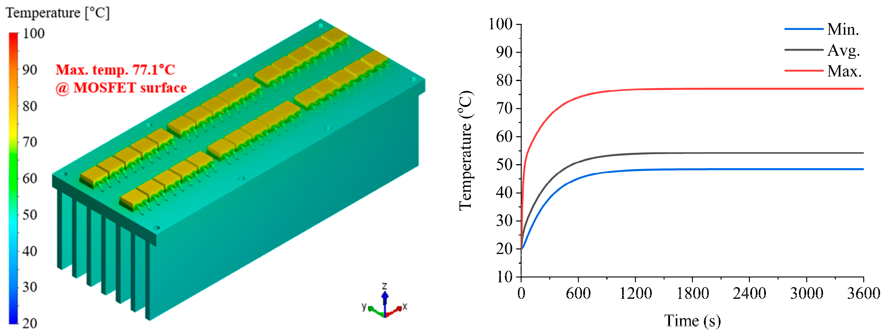
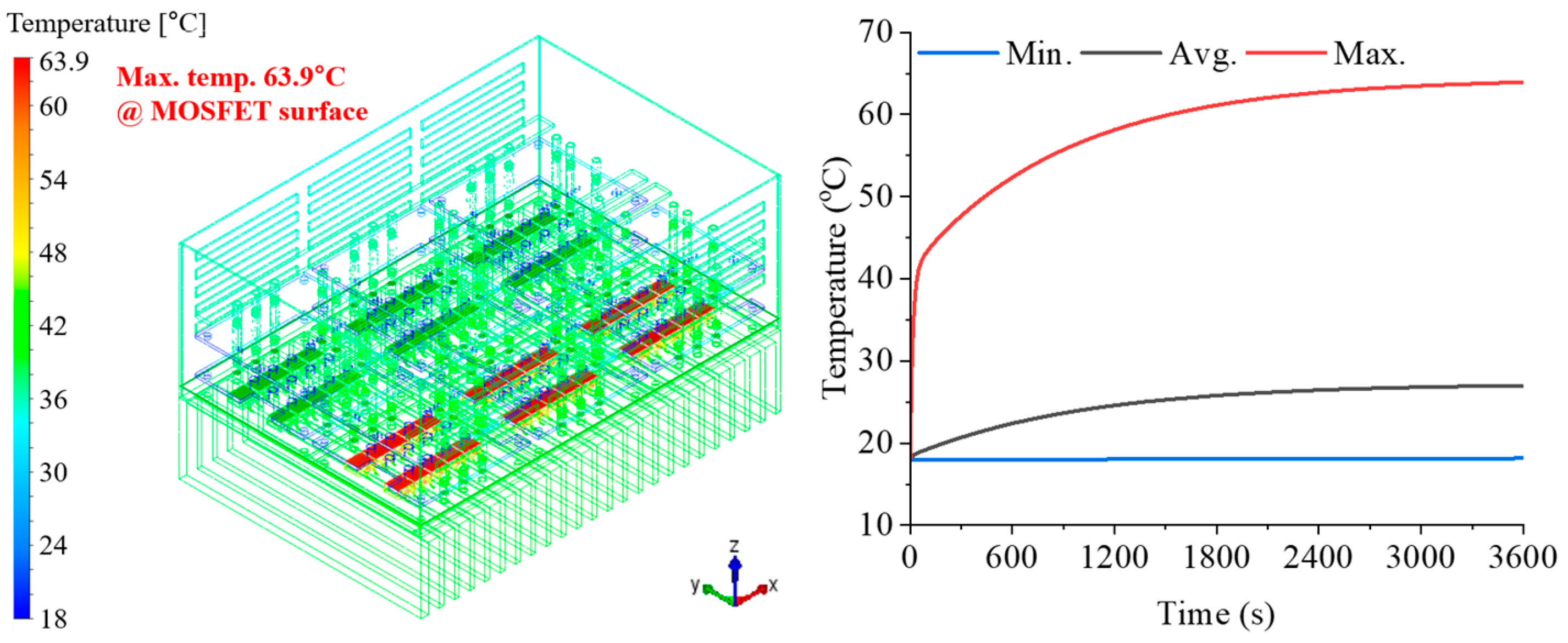
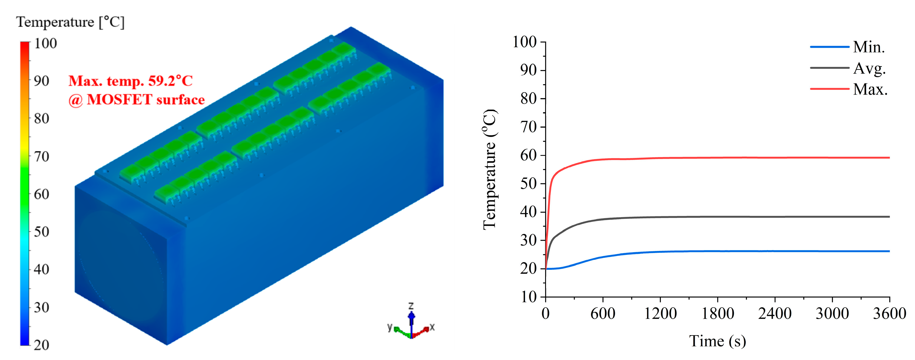
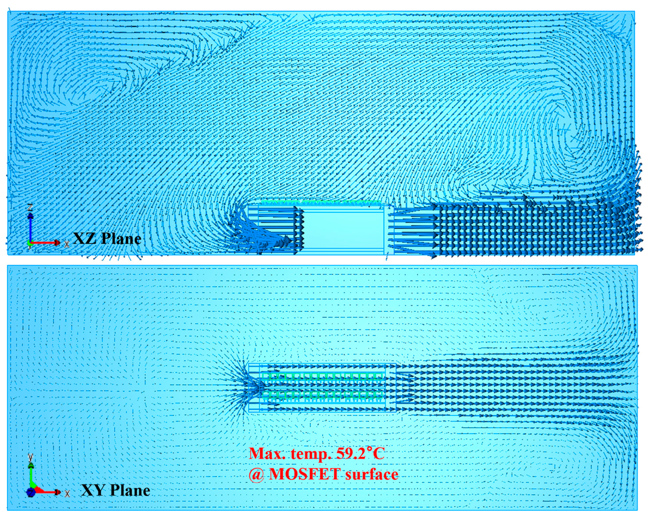
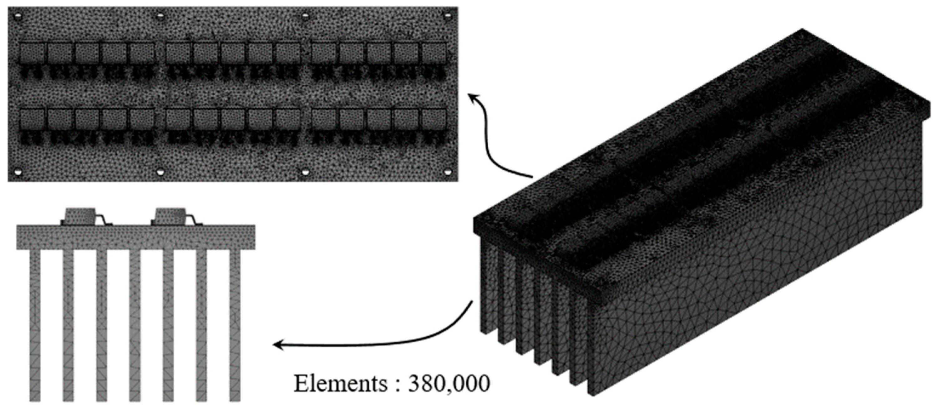
3.1.2. CFD Analysis
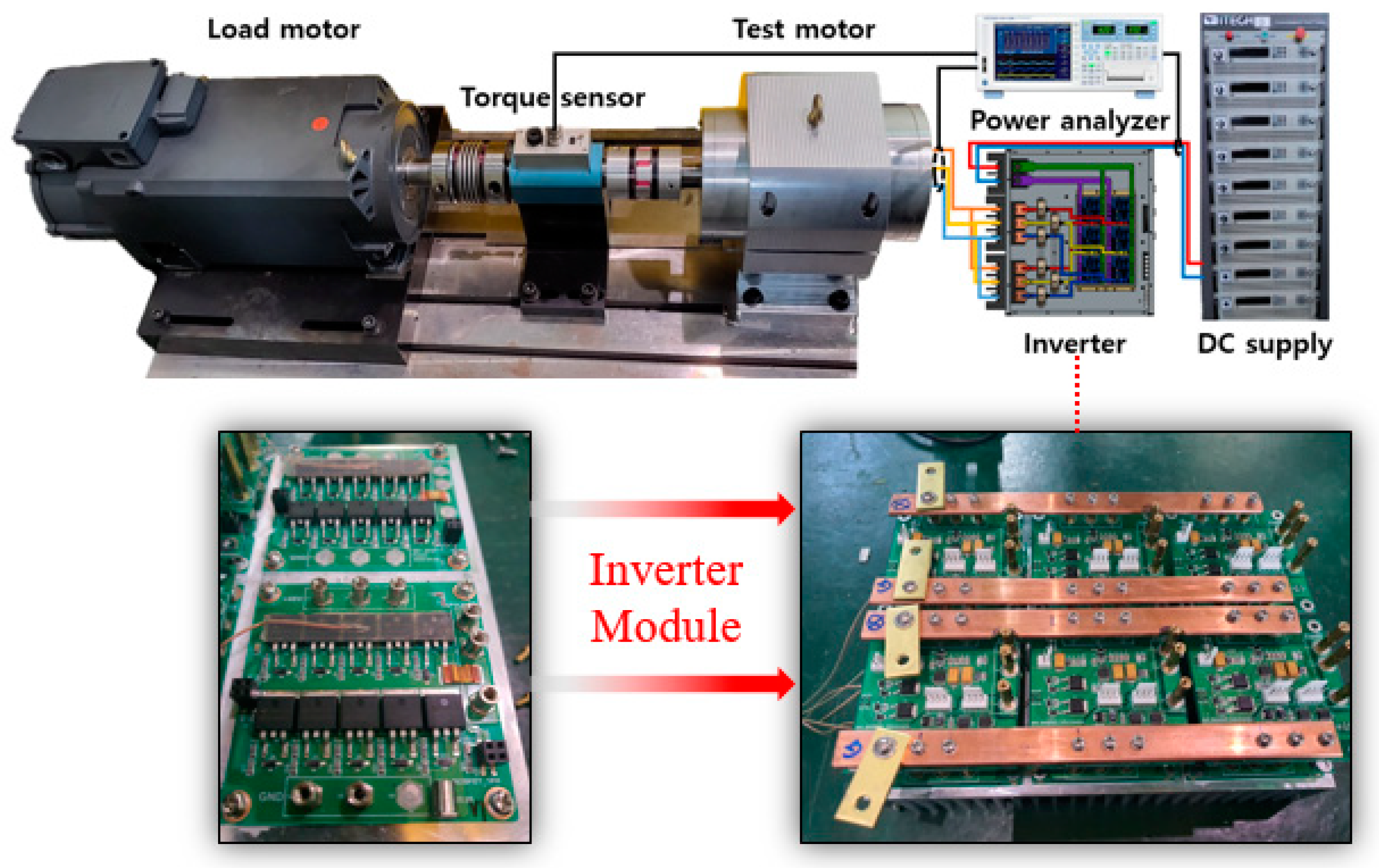
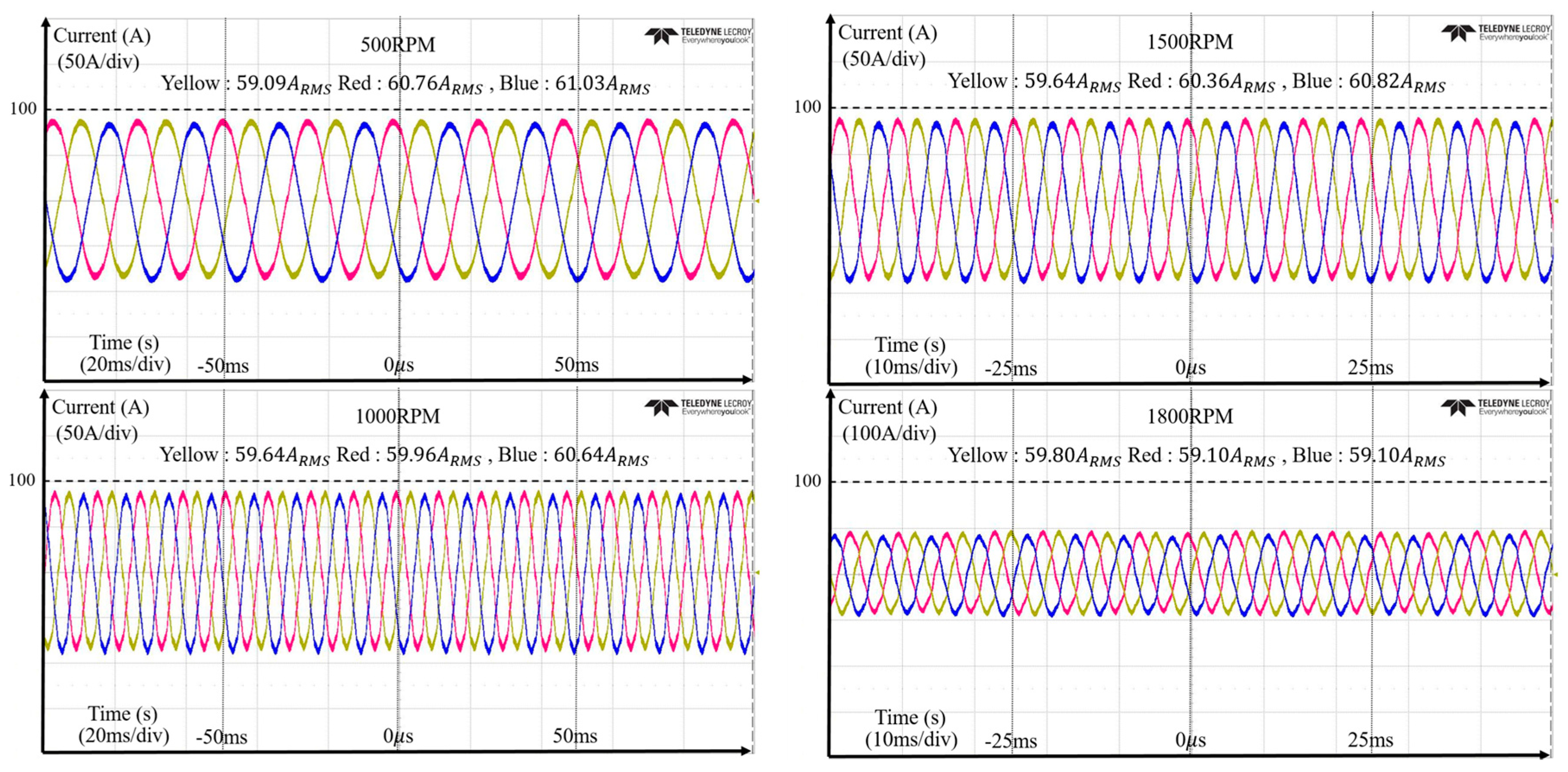
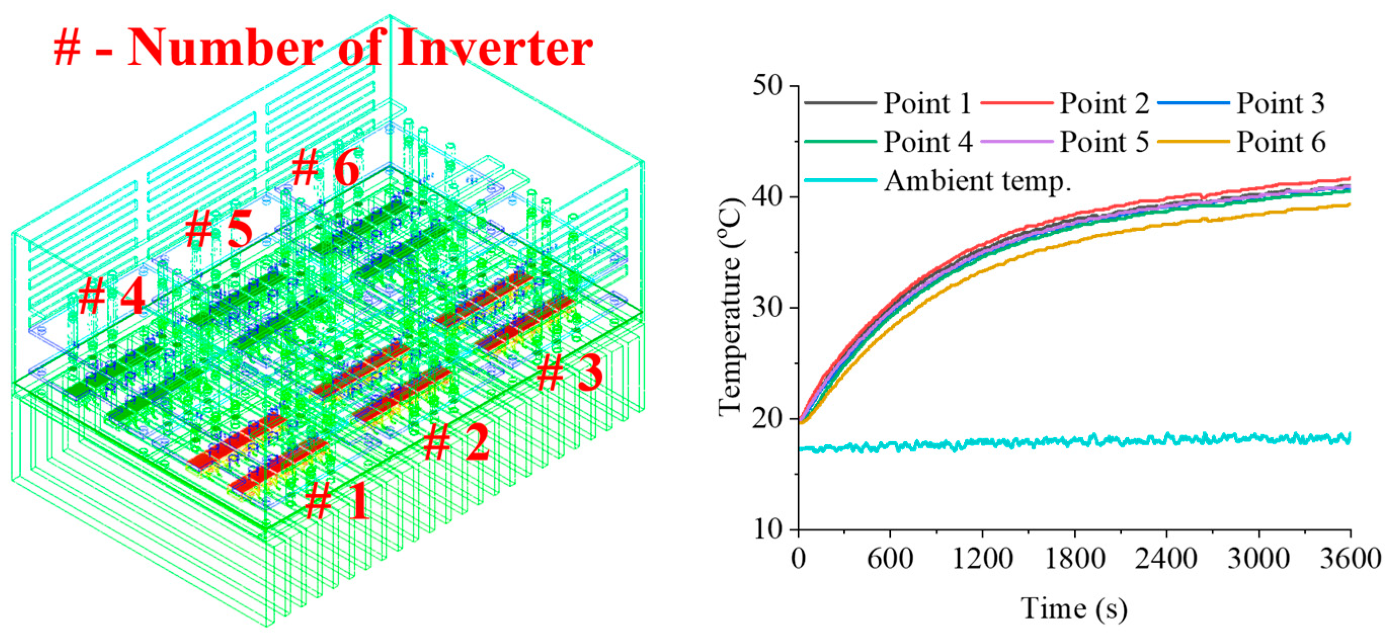
3.2. Experimental Verification
4. Conclusions
Author Contributions
Funding
Conflicts of Interest
References
- Quere, C.; Andrew, R.; Friedlingstein, P.; Kaushik, R.; Sitch, S.; Hauck, J.; Pongratz, J.; Picker, P.; Ivar, K.; Peters, G.; et al. Global Carbon Budget 2018. Earth Syst. Sci. Data 2018, 10, 2147–2194. [Google Scholar] [CrossRef]
- Tan, Y.; Nookuea, W.; Li, H.; Thorin, E.; Yan, J. Property impacts on Carbon Capture and Storage (CCS) processes: A review. Energy Convers. Manag. 2016, 118, 204–222. [Google Scholar] [CrossRef]
- Barbara, B.; Maurizio, A.; Emilio, A.; Dario, B. Process analysis of a molten carbonate fuel cell on-board application to reduce vessel CO2 emissions. Chem. Eng. Process. Process Intensif. 2023, 190, 109415. [Google Scholar]
- Kaushik, R. Present Status and Future Trends in Electric Vehicle Propulsion Technologies. J. Emerg. Sel. Top. Power Electron. IEEE 2013, 1, 3–10. [Google Scholar]
- Dinesh, K.; Firuz, Z. A Comprehensive Review of Maritime Microgrids: System Architectures, Energy Efficiency, Power Quality, and Regulations. IEEE Access 2019, 7, 67249–67277. [Google Scholar]
- Husain, I.; Ozpineci, B.; Islam, M.S.; Gurpinar, E.; Su, G.J.; Yu, W.; Chowdhury, S.; Xue, L.; Rahman, D.; Sahu, R. Electric Drive Technology Trends, Challenges, and Opportunities for Future Electric Vehicles. Proc. IEEE 2021, 109, 1039–1059. [Google Scholar] [CrossRef]
- Liu, Z.; Wu, J.; Hao, L. Coordinated and fault-tolerant control of tandem 15-phase induction motors in ship propulsion system. IET Electr. Power Appl. 2018, 12, 91–97. [Google Scholar] [CrossRef]
- Sandro, C.; Daniel, F.; Roberto, P.; Mauro, B.; Mario, M.; Alberto, T. A Fully-Integrated Fault-Tolerant Multi-Phase Electric Drive for Outboard Sailing Boat Propulsion. In Proceedings of the 21st European Conference on Power Electronics and Applications, Genova, Italy, 3–5 September 2019. [Google Scholar]
- Mohamed, A.F.; Julien, C.; Kritika, D.; Yassine, B.; Mohamed, E.B.; Omar, H. Multiphase Motors and Drive Systems for Electric Vehicle Powertrains: State of the Art Analysis and Future Trends. Energies 2023, 16, 768. [Google Scholar]
- Matus, K.; Ludek, B.; Petr, B. Compensation methods of interturn short-circuit faults in dual three-phase PMSM. In Proceedings of the IECON 2020 The 46th annual Conference of the IEEE Industrial Electronics Society, Singapore, 18–21 October 2020; pp. 4833–4838. [Google Scholar]
- Sun, W.; Liu, J.; Wei, S.; Gong, X. Heat dissipating structure design of an inverter with direct-cooling IGBT module for EV. In Proceedings of the IEEE Conference and Expo Transportation Electrification Asia-Pacific (ITEC Asia-Pacific), Beijing, China, 3 September–31 November 2014. [Google Scholar]
- Aldo, K.; Andrea, C.; David, S.; Martin, S.; Markus, M.; Carlos, M. Evolution and Modern Approaches for Thermal Analysis of Electrical Machines. IEEE Trans. Ind. Electron. 2009, 56, 871–882. [Google Scholar]
- Ye, J.; Yang, K.; Ye, H.; Emadi, A. A Fast Electro-Thermal Model of Traction Inverters for Electrified Vehicles. IEEE Trans. Power Electron. 2017, 32, 3920–3934. [Google Scholar] [CrossRef]
- Dong, J.; Huang, Y.; Jin, L.; Lin, H.; Yang, H. Thermal Optimization of a High-Speed Permanent Magnet Motor. IEEE Trans. Magn. 2014, 50, 7018504. [Google Scholar] [CrossRef]
- Ren, Y.; Xu, M.; Zhou, J.; Lee, F.C. Analytical loss model of Power MOSFET. IEEE Trans. Power Electron. 2006, 21, 310–319. [Google Scholar]
- Shen, Z.J.; Xiong, Y.; Cheng, X.; Fu, Y.; Kumar, P. Power MOSFET Switching Loss Analysis: A New Insight. In Proceedings of the Conference Record of the 2006 IEEE Industry Applications Conference Forty-First IAS Annual Meeting, Tampa, FL, USA, 8–12 October 2006. [Google Scholar]
- Utkarsh, J.; Faisal, M.; Hamid, A.M.; Peyush, P.; Mayank, C.; Sima, D. A Method for Selection of Power MOSFETs to Minimize Power Dissipation. Electronics 2021, 10, 2150. [Google Scholar]
- Toni, L.; Reinhold, E. Current sharing of paralleled power MOSFETs at PWM operation. In Proceedings of the IEEE Power Electronics Specialists Conference 2016, Jeju, South Korea, 18–22 June 2006. [Google Scholar]
- «POWERFORGE, Multi-Level by Design» Power Design Technologies SA. Available online: https://powerforge.powerdesign.tech (accessed on 30 September 2023).
- «PLECS, The Simulation Platform for Power Electronic Systems» Plexim. Available online: https://www.powersimtech.com (accessed on 30 September 2023).
- «Autodesk Simulation CFD». Available online: https://help.autodesk.com (accessed on 30 September 2023).
- «Altair CFD». Available online: https://www.altair.com (accessed on 30 September 2023).
- Singh, Y.; Bhattacharyya, S.K.; Idichandy, V.G. CFD approach to modelling, hydrodynamic analysis and motion characteristics of a laboratory underwater glider with experimental results. J. Ocean Eng. Sci. 2017, 2, 90–119. [Google Scholar] [CrossRef]
- Mo, Q.; Guan, H.; He, S.; Liu, Y.; Guo, R. Guidelines for the computational domain size on an urban-scale VAWT. J. Phys. 2021, 1820, 012177. [Google Scholar] [CrossRef]
- Jochen, F.; Christopher, M.; Wolfgang, R.; Lionel, T. Highly resolved large-eddy simulation of separated flow in a channel with streamwise periodic constriction. J. Fluid Mech. 2005, 526, 19–66. [Google Scholar]
- Frank, P. Incropera’s Principles of Heat and Mass Transfer; Global Ed.; Wiley: Hoboken, NJ, USA, 2017. [Google Scholar]
- Buchmann, H.-F. Properties and Applications of Epoxy Moulding Compounds, 1st ed.; Duresco GmbH: Witterswil, Switzerland, 2019; pp. 1–13. [Google Scholar]
- Lee, S.H.; Doe, J.K.; Song, H.H.; Kim, S.W.; Kang, K.H.; Lee, W.S. Thermophysical poperties of epoxy molding compound for microelectronic packaging. In Proceedings of the Seventeenth European Conference on Thermophysical Properties (ECTP), Bratislava, Slovak Republic, 5–8 September 2005. [Google Scholar]
- Caplinq Blog. Available online: https://www.caplinq.com/blog/heat-capacity-of-epoxy-molding-compound_102/ (accessed on 25 September 2023).
- Tang, H.; Li, W.; Li, J.; Gao, H.; Wu, Z.; Shen, X. Calculation and Analysis of the Electromagnetic Field and Temperature Field of the PMSM Based on Fault-Tolerant Control of Four-Leg Inverters. IEEE Trans. Energy Convers. 2020, 35, 2141–2151. [Google Scholar] [CrossRef]
- Li, W.; Li, L.; Gao, H.; Li, D.; Zhang, X.; Fan, Y. Influence of direct-connected inverter with one power switch open circuit fault on electromagnetic field and temperature field of permanent magnet synchronous motor. IET Electr. Power Appl. 2018, 12, 815–825. [Google Scholar] [CrossRef]


| Cell | Device | Package | Number of MOSFETs in | ||
|---|---|---|---|---|---|
| Cell 1 Bottom | Si MOSFET (CSD19536KTT) | TO-263 | 5 (Connected in Parallel) | 100 V | 272 A |
| Cell 1 Top | 5 (Connected in Parallel) | ||||
| Cell 2 Bottom | 5 (Connected in Parallel) | ||||
| Cell 2 Top | 5 (Connected in Parallel) | ||||
| Cell 3 Bottom | 5 (Connected in Parallel) | ||||
| Cell 3 Top | 5 (Connected in Parallel) |
| Parameters | Symbols | Values |
|---|---|---|
| DC-link voltage | 48 V | |
| Rated speed | RPM | 1800 RPM |
| Rated torque | 16 | |
| Number of poles | - | 10 |
| Switching frequency | Hz | 10,000 Hz |
| Direct-axis inductance | H | 76.5 μH |
| Quadrature-axis inductance | H | 81.4 μH |
| Stator resistance | Ω | 17.1 mΩ |
| Flux linkage | Wb | 24.3 mWb |
| Cell | Conduction Type | (W) | ||||
|---|---|---|---|---|---|---|
| Cell 1 Bottom | ||||||
| Forward | 50.5 | 1.93 | 0.449 | 1.01 | 3.39 | |
| Reverse | 19.4 | 0.287 | 0.304 | - | 0.591 | |
| Total | 54.1 | 2.217 | 0.753 | 1.01 | 3.981 |
| Conditions | Condition Details | Values |
|---|---|---|
| Governing equations | Equations | Navier–Stokes eq. |
| Energy equation | Advective diffusive | |
| Turbulence modeling | N/A (laminar) | |
| Boundary conditions | Domain walls with radiation | -- |
| HTC (heat transfer coefficient) | ||
| Temperature | 27 (300 K) | |
| Environmental conditions (air) | Density | 1.225 |
| Dynamic viscosity | 1.781 | |
| Temperature | 27 (300 K) | |
| Convection effect | HTC (heat transfer coefficient) | |
| Temperature | 27 (300 K) | |
| Radiation effect | Emissivity | |
| Y+ check | <20.0 | 1.5 |
| Mesh type/number | Boundary layer mesh | 1.2 M< |
| Heat density | Each per MOSFET | 9.768 (W/mm3) |
| Analysis type | Transient (time step) | 1 s |
| Material | Density (kg/ | Thermal Conductivity (W/m) | Specific Heat (J/kg) |
|---|---|---|---|
| Aluminum | 2707 | 204 | 896 |
| Copper | 8934 | 380 | 380 |
| EMC | 1900 [27] | 0.8 [28] | 800 [29] |
| FR-4 | 1820 | 0.29 | 1150 |
| Iron | 7849 | 59 | 460 |
| Parameters | Symbols | Values |
|---|---|---|
| Power | kW | 10 kW |
| Rated speed | RPM | 1800 RPM |
| Rated torque | 53.05 | |
| Number of poles | - | 10 |
| Rated current | 200 | |
| Direct-axis inductance | H | 36.66 μH |
| Quadrature-axis Inductance | H | 36.05 μH |
| Quadrature-axis Flux linkage | Wb | 25.19 mWb |
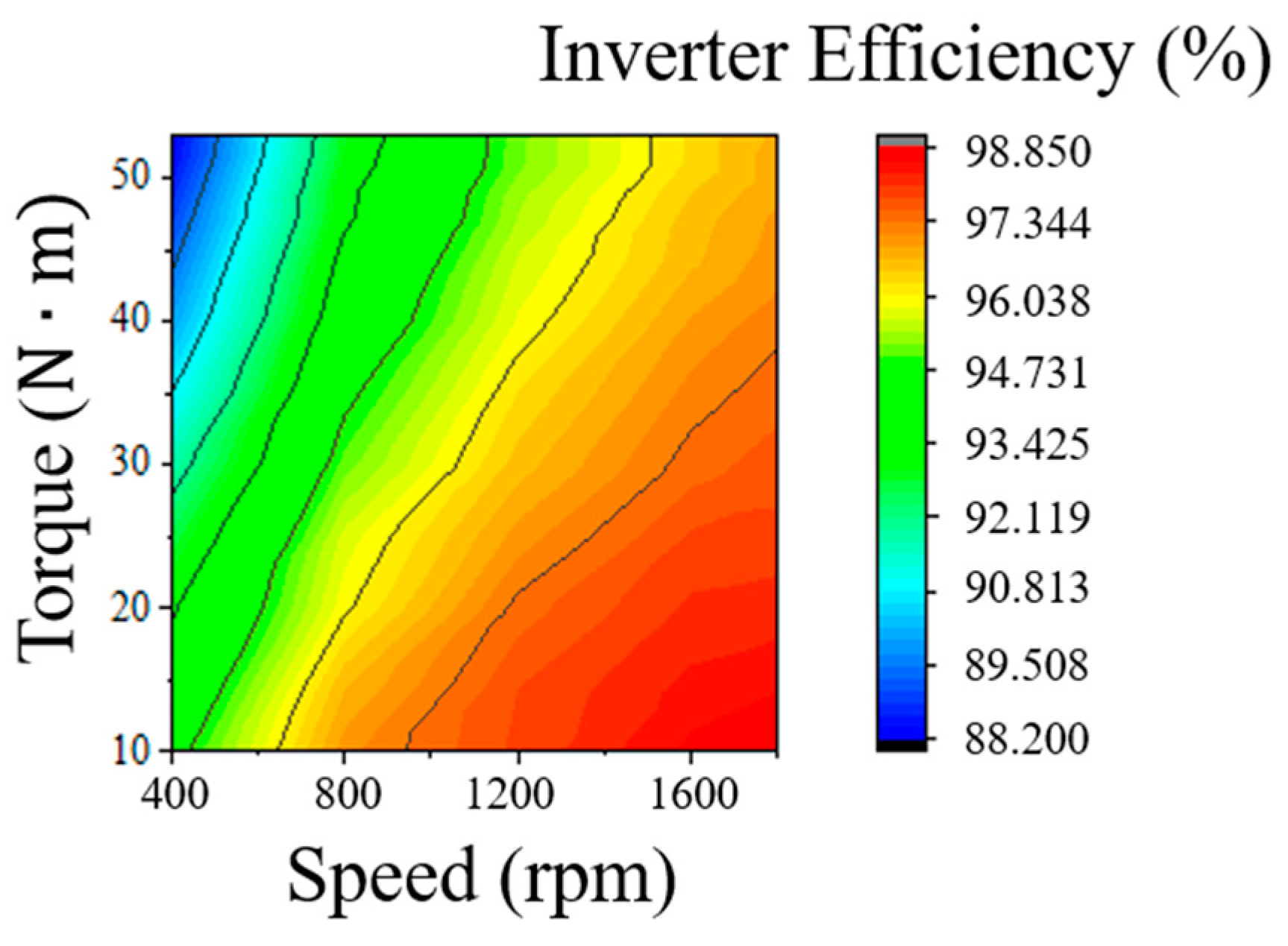
| 10 kW | U_1 | U_2 | U_3 | I_1 | I_2 | I_3 | P | Efficiency |
|---|---|---|---|---|---|---|---|---|
| 1800 RPM | 40.32 | 40.61 | 40.40 | 188.29 | 189.20 | 190.26 | 10.9k | 96.746 |
| 40.33 | 40.62 | 40.41 | 188.29 | 189.21 | 190.27 | 10.9k | 96.743 | |
| 40.33 | 40.62 | 40.40 | 188.28 | 189.21 | 190.2 | 10.9k | 96.763 |
Disclaimer/Publisher’s Note: The statements, opinions and data contained in all publications are solely those of the individual author(s) and contributor(s) and not of MDPI and/or the editor(s). MDPI and/or the editor(s) disclaim responsibility for any injury to people or property resulting from any ideas, methods, instructions or products referred to in the content. |
© 2023 by the authors. Licensee MDPI, Basel, Switzerland. This article is an open access article distributed under the terms and conditions of the Creative Commons Attribution (CC BY) license (https://creativecommons.org/licenses/by/4.0/).
Share and Cite
Park, J.-S.; Lee, T.-W.; Lee, J.-W.; Park, B.-G.; Kim, J.-W. Optimization of Multi-Phase Motor Drive System Design through Thermal Analysis and Experimental Validation of Heat Dissipation. Electronics 2023, 12, 4177. https://doi.org/10.3390/electronics12194177
Park J-S, Lee T-W, Lee J-W, Park B-G, Kim J-W. Optimization of Multi-Phase Motor Drive System Design through Thermal Analysis and Experimental Validation of Heat Dissipation. Electronics. 2023; 12(19):4177. https://doi.org/10.3390/electronics12194177
Chicago/Turabian StylePark, Jun-Shin, Tae-Woo Lee, Jae-Woon Lee, Byoung-Gun Park, and Ji-Won Kim. 2023. "Optimization of Multi-Phase Motor Drive System Design through Thermal Analysis and Experimental Validation of Heat Dissipation" Electronics 12, no. 19: 4177. https://doi.org/10.3390/electronics12194177
APA StylePark, J.-S., Lee, T.-W., Lee, J.-W., Park, B.-G., & Kim, J.-W. (2023). Optimization of Multi-Phase Motor Drive System Design through Thermal Analysis and Experimental Validation of Heat Dissipation. Electronics, 12(19), 4177. https://doi.org/10.3390/electronics12194177