Inverter Fault Diagnosis for a Three-Phase Permanent-Magnet Synchronous Motor Drive System Based on SDAE-GAN-LSTM

Abstract

In this study, a novel intelligent inverter fault diagnosis approach based on a stacked denoising autoencoder–generative adversarial network–long short-term memory (SDAE-GAN-LSTM) under an imbalanced sample is proposed for a three-phase permanent-magnet synchronous motor (PMSM) drive system. The proposed method can address the problem of unbalanced fault data samples and improve the accuracy of fault classification. Concretely speaking, firstly, the stacked denoising autoencoder (SDAE) is pre-trained to obtain the optimum decoder network. Afterward, a new generator of generative adversarial networks (GANs) is designed to generate high-quality samples by migrating the pre-trained optimal decoder network to the hidden layer and output layer of the generator of GANs. Additionally, a new model of long short-term memory (LSTM) based on the second discriminator of the GANs is presented for fault diagnosis. The generator of GANs is cross-trained using the reconstruction error gained by SDAE and the fault diagnosis error obtained by LSTM, resulting in the generation of high-quality samples for fault discrimination. Simulation and experimental results demonstrate the effectiveness of the proposed fault diagnosis approach, and the average fault identification accuracy reaches 98.63%.

1. Introduction

The three-phase permanent-magnet synchronous motor (PMSM) drive systems are widely utilized in manufacturing, electric vehicle applications, the metallurgical industry, etc., due to their high reliability and efficiency [1,2]. The PMSM faults cause the deteriorating performance of the device and affect the safe operation of equipment. More seriously, faults can even cause significant safety and casualty accidents. Therefore, timely and accurate fault diagnosis of such machinery is attracting the attention of scholars to reduce unexpected downtime, economic losses, and personal injuries [3]. The fault diagnosis model is established through data feature extraction technology [4,5,6]. Finally, fault diagnosis is completed using machine learning techniques [7] or deep learning methods.

As known to us all, the fault diagnosis model is established through data feature extraction technology [8]. Fault signals of many mechanical systems are typically non-stationary time series because the fault is caused by the accumulation of degradation over a long period of time. They are also long-term-dependent in the temporal domain and interrelated in the spatial dimension. In reference [9], a deep learning-based observer, which combines the CNN and the LSTM, was employed in the fault detection of the nonlinear driving control system. Yixuan Mao et al. [10] came up with a novel hybrid approach based on an LSTM neural network and a support vector machine (LSTM-SVM), which revealed great performance in mooring failure detection. In reference [11], a dual deep learning reference classifier, utilizing CNN and LSTM, was specifically designed for the classification of synchronous motor electrical faults. Haitao Zhao et al. [12] used the LSTM neural network to directly classify raw processed data, which provided good fault diagnosis performance. In reference [13], an LSTM-regulated deep residual network was proposed for data-driven fault detection, which achieved good results in the accuracy of detection. Hence, the fault diagnosis problem can be converted to time series identification. LSTM received more scholarly attention when it was proposed due to its exemplary recognition and identification capabilities for time series. Reference [14] introduced a data-driven fault diagnosis method that leveraged long short-term memory (LSTM) networks for detecting multiple open-circuit switch faults in the back-to-back converter of a doubly fed induction generator-based wind turbine system. Ping Zou et al. [15] used LSTM to adaptively fuse IMF component information and extract features from rotating electrical machines to intelligently classify and recognize bearing status. Admittedly, these existing methods have high accuracy, but it is undeniable that the results depend on the huge amount of balanced data. Simultaneously, only a few of the samples are normal, and most of the samples are faulty due to the high-reliability design of the PMSM drive system. That is, the sample is distributed in a long tail, which is small and unbalanced.

With the rapid development of data-driven artificial intelligence, generative adversarial networks (GANs) were proposed by researchers in 2014 [16]. GAN has been widely used in various fields because of its powerful ability to learn the original sample distribution and generate similar data distributions [17]. Hence, many scholars have employed GAN to solve the problem of unbalanced and small samples. Reference [18] proposed a fault diagnosis method based on LSTM and GAN for wind turbines. GAN uses the generator to solve the problem of insufficient data labels, and the Bayesian optimized LSTM prediction accuracy is better. To meet the large number of requirements for intermittent fault diagnosis and degradation assessment, the LSTM-GAN-based method is presented in reference [19]. Although these methods have obtained good fault diagnosis results across diverse systems, the authors in this paper have identified suboptimal performance of the LSTM-GAN-based method in fault diagnosis for PMSM. The accuracy is only about 94%. As a result, the main issue of this paper is how to improve the accuracy of fault diagnosis.

As known to us all, the performance of fault diagnosis depends on both feature extraction and pattern recognition [20,21,22]. In the existing references [23,24,25,26], it can be seen that combining multiple intelligent feature extraction methods from larger feature quantities can better improve the accuracy of the classification model. Consequently, one can see that effective means of feature extraction may contribute to GAN-LSTM-based fault diagnosis. In reference [27], the autoencoder (AE) is used to perform critical temporal feature extraction and dimension reduction; thus, the fault diagnosis performance of the LSTM-GAN-based method is improved. However, the AE can only approximately copy inputs similar to the training data; that is, it is a compressed representation of the data and easily causes overfitting problems. To solve this problem, DAE [28] is proposed to enhance the robustness of the trained encoder by adding noise to the input data. On this basis, SDAE [29] is presented to obtain better data representation with the deep neural network. Recently, DAE and SDAE were employed with other deep learning methods for diagnosis, achieving good applicational progress [30,31]. Unfortunately, the fault diagnosis design of the structure that combined GAN-LSTM with SDAE has not been widely applied in practice.

Considering the above shortcomings and advantages, this paper proposes a fault diagnosis method based on SDAE-GAN-LSTM. Among the three neural network frameworks proposed in this paper, the advantage of SDAE in extracting deep features from nonlinear data is fully utilized, while the ability of LSTM to deal with the dependence of time series information is fully utilized for effective classification and recognition. Furthermore, the proposed method designed a new generator to generate higher-quality samples, which can be applied to fault identification. Meanwhile, the training of the generator is optimized by utilizing the ability of SDAE to extract deep fault features and the fault diagnosis error of LSTM to generate high-quality samples. Therefore, the fault diagnosis accuracy of the three-phase PMSM inverter is improved.

The main innovations of this paper are as follows:

• We designed a new generator to generate fault features rather than fault data. First, stacked denoising autoencoders are pre-trained to obtain optimal parameters. Then, the optimized parameters are migrated to the generator layer of GAN, where the generated fault features are decoded to obtain fake samples.
• We designed a new discriminator. The LSTM fault diagnosis model is added to the real discriminator of the traditional GAN network, which overcomes the defect of the traditional GAN not filtering low-quality samples. The new discriminator needs to identify the authenticity of the sample while considering the results of the fault diagnosis of the generated sample.
• Furthermore, the model demonstrates enhanced capabilities in generating samples and conducting fault diagnosis. Improvements have been achieved in the sample generation ability of the generator, the discriminator’s discriminative performance, and the fault diagnosis capability of the LSTM.

The rest of this article is arranged as follows. Section 2 introduces the basic theory of SADE, GAN, and LSTM; Section 3 elaborates on the imbalanced sample data fault diagnosis algorithm based on SDAE-GAN-LSTM; Section 4 illustrates the simulation results; Section 5 presents the conclusion.

2. Theoretical Background

The theoretical background will be provided in this section, including the stacked denoising autoencoder, LSTM, and GAN.

2.1. Stacked Denoising Autoencoder

An autoencoder (AE) is a deep learning model consisting of an encoder network and a decoder network. Its primary objective is to preserve the input distribution as closely as possible to the output. It excels at feature extraction from input data. Subsequently, the network parameters of the AE undergo optimization through a process known as fine-tuning. The denoising autoencoder (DAE) is designed to filter input data affected by noise, thereby enhancing the network’s robustness. The stacked denoising autoencoder (SDAE) is constructed by combining multiple denoising autoencoders, as illustrated in Figure 1. Within the SDAE architecture, the output of the encoder in $DA{E}_n$ serves as the input of the decoder in $DA{E}_{n+1}$. Through multiple rounds of pre-training, the parameters of the end of the DAE are iteratively improved. Upon completion of SDAE pre-training, the optimal network parameters are ascertained.

Figure 1. The structure of SDAE.

In the autoencoder, the original input, denoted as x, is passed through the encoder to the hidden layer to obtain the feature h. Additionally, the output value $\widehat{x}$ is obtained by reconstructing the hidden layer features via the decoder. The mathematical expression of the autoencoder network is expounded through Equations (1) and (2):

$$h=\sigma \left(\omega ·x+b\right)$$

(1)

$$\begin{array}{c}\hfill \widehat{x}=\sigma \left({\omega }^{\prime }·h+b^{\prime }\right)\end{array}$$

(2)

where $\sigma$ denotes the nonlinear activation function sigmoid, $\omega$ and ${\omega }^{\prime }$ are the weight matrices, b and $b^{\prime }$ are the bias vectors. h is obtained by encoding the input x, and $\widehat{x}$ is the reconstruction value.

The network parameters of the AE are optimized by minimizing the error, denoted as J, which measures the distance between the input and the reconstructed value. This optimization process is formally represented in Equation (3).

$$argmin\left(J(x,\widehat{x})\right)=\sum _k^n{∥x-\widehat{x}∥}_2^2$$

(3)

where k is the number of samples. In the stacked denoising autoencoder, Equation (3) is also adopted as the loss function.

2.2. Generative Adversarial Network

The standard generative adversarial network (GAN) consists of a generator network and a discriminator network. The architectural framework of the GAN is illustrated in Figure 2. The role of the generator network is used to generate samples that are consistent with the sample distribution, while the discriminator network is used to identify the authenticity of the generated samples. In the GAN network, the generator employs Gaussian-distributed random noise, denoted as z, to synthesize samples $G\left(z\right)$ that are consistent with the distribution of real samples. Subsequently, the discriminator assesses both the generated and real samples, while the generator parameters are updated accordingly. This adversarial interplay between the generator and discriminator persists until the achievement of the global optimum. The optimization objective of the discriminator is to maximize Equation (4):

$$D\_loss=logD\left(x\right)+log(1-D(G\left(z\right)\left)\right)$$

(4)

Figure 2. The structure of GAN.

The optimization goal of the generator is to minimize Equation (5):

$$G\_loss=log(1-D(G\left(z\right)\left)\right)$$

(5)

Based on the loss functions, $D\_loss$ and $G\_loss$, the training process of the standard GAN continues until the attainment of the global optimum, referred to as $D\_loss=G\_loss=0.5$, is completed. It is at this juncture that the standard GAN achieves a Nash equilibrium state, providing evidence that the generated samples closely resemble the real samples.

2.3. Long Short-Term Memory

The long short-term memory (LSTM) network represents an enhanced version of the recurrent neural network (RNN). The LSTM adds three gate units: the forget gate, the input gate, and the output gate, which collectively heighten the network’s capacity to retain crucial feature information [32]. By incorporating memory units to capture long-term dependencies between time series information, LSTM can effectively address the issues of gradient explosion and gradient disappearance phenomena. As shown in Figure 3, the structure of LSTM incorporates five activation functions, among which, $f_t$, $i_t$, and $O_t$ are all sigmoid functions, while $g_t$ and $m_t$ are tanh functions.

Figure 3. The structure of LSTM.

First, the role of the forget gate is to selectively forget irrelevant information from the memory cells; the mathematical expression for this process is provided in Equation (6):

$$f_t=\sigma \left({\omega }_f·x_t+{\omega }_f·h_{t-1}+b_f\right)$$

(6)

where ${\omega }_f$ and $b_f$ denote the weight matrix and bias of the forget gate, respectively. $h_{t-1}$ is the state of the last hidden layer and $x_t$ is the input.

Simultaneously, the purpose of the input gate is to determine and reserve relevant information. The mathematical expression for this function is represented in Equation (7):

$$i_t=\sigma \left({\omega }_i·x_t+{\omega }_i·h_{t-1}+b_i\right)$$

(7)

where ${\omega }_i$ and $b_i$ denote the weight matrix and bias of the input gate, respectively.

Furthermore, the mathematical representation for the input candidate information $g_t$ is detailed in Equation (8):

$$g_t=tanh\left({\omega }_g·x_t+{\omega }_g·h_{t-1}+b_g\right)$$

(8)

The current memory cell state, denoted as $C_t$, can be formally expressed in Equation (9):

$$C_t=C_{t-1}\odot f_t+g_t\odot i_t$$

(9)

Additionally, the function of the output gate is to output the characteristics of the hidden layer in a non-linearly activated manner. The mathematical representation of this operation is provided in Equation (10):

$$O_t=\sigma \left({\omega }_o·x_t+{\omega }_o·h_{t-1}+b_o\right)$$

(10)

where ${\omega }_o$ and $b_o$ denote the weight matrix and bias of the output gate, respectively.

Moreover, $h_t$ represents the subsequent updated hidden state, and the mathematical expression is presented in Equation (11):

$$h_t=O_t\odot tanh\left(C_t\right)$$

(11)

A Softmax classifier is implemented on top of the LSTM layer. This paper trains the Softmax classifier using the state $H_t=\left\{h_1,h_2,\cdots h_N\right\}$ and data label $\left\{1,2,\cdots N\right\}$. The optimization of the Softmax classifier is to minimize the loss function Equation (12). The specific optimization process will be described in Section 3.

$$L_{LSTM-\mathrm{loss}}=J\left(\Theta \right)$$

(12)

where $\Theta =\left\{{\theta }_f,{\theta }_i,{\theta }_g,{\theta }_O\right\}$ is the parameters of the LSTM. To meet the requirements of LSTM for fault diagnosis, the network parameters are constantly fine-tuned by backpropagation.

3. Fault Diagnosis Algorithm Based on SDAE-GAN-LSTM

Due to the high reliability and highly stringent design principles of PMSM, the motor drive systems typically operate under normal conditions during their operational phases. It is worth mentioning that the fault signals are characterized by a long-tailed distribution, which brings a challenge to data-driven intelligent fault diagnosis technology due to the imbalanced sample distribution. In this paper, the advantages of three neural network frameworks are combined to address this issue. First, this paper harnesses the deep feature extraction capabilities of SDAE to extract nonlinear features from the data. Second, this experiment utilizes GAN to tackle the problem of imbalanced samples. Finally, LSTM networks are employed to process time series data and perform classification recognition. The basic principles of the specific model and the introduction of the diagnostic process are elucidated in this section.

3.1. Design of Generator

In this paper, a novel generator is designed for the generation of features in imbalanced sample datasets. The generator network is optimized by using real features so that the generator can generate the features of the imbalance samples. Then, the generated features are decoded to generate samples. To initiate this process, a random noise distribution, denoted as z, is used as the input of the generator to obtain $X_{feature-fake}$. Its process can be expressed as Equations (13) and (14):

$$h_z=f_{{\theta }_{G1}}\left(z\right)=\mathrm{Re}lu\left({\omega }_z·z+b_z\right)$$

(13)

$$\begin{array}{c}\hfill X_{feature-fake}=f_{{\theta }_{G2}}\left(h_z\right)=\sigma \left({\omega }_G·z+b_G\right)\end{array}$$

(14)

where ${\theta }_{G1}=\left\{{\omega }_{\mathrm{z}},{\mathrm{b}}_z\right\}$ and ${\theta }_{G2}=\left\{{\omega }_G,{\mathrm{b}}_G\right\}$ are the weight matrix and bias of the generator input layer and hidden layer, respectively. Both $\sigma$ and $\mathrm{Re}Lu$ are activation functions.

To ensure that the generated sample $X_{fake}$ aligns with the requirements of fault diagnosis, this paper uses SDAE to decode $X_{feature-fake}$. The SDAE is trained in this study by using the imbalanced sample $X_{real}$. The detailed training process is outlined as follows:

Step 1:

The original signal $X_{real}$ is processed by adding noise to obtain the input ${\stackrel{⌢}{X}}_{real}$, which makes the decoder network robust.

Step 2:

According to Equation (15), the input ${\stackrel{⌢}{X}}_{real}$ is encoded to obtain the first layer feature: ${X_{feature-real}}_{{}_1}$;

$$\begin{array}{c}\begin{array}{c}\begin{array}{c}{X_{feature-real}}_1=f\left({\stackrel{⌢}{X}}_{real}\right)=\sigma ({\omega }_1·{\stackrel{⌢}{X}}_{real}+b_1)\end{array}\end{array}\end{array}$$

(15)

where ${\theta }_1=\left\{{\omega }_1,{\mathrm{b}}_1\right\}$ are the weight matrix and bias of the first $DA{E}_1$.

Step 3:

Then ${X_{feature-real}}_{{}_1}$ is used as the input of the second $DA{E}_2$. Repeat Step 2–Step 3 until the ${X_{feature-real}}_N$ is decoded by the N-th $DA{E}_N$. According to Equation (16), the ${X_{feature-real}}_N$ is decoded to obtain the output ${\widehat{X}}_{real}$.

$$\begin{array}{c}\hfill \begin{array}{c}\hfill {\widehat{X}}_{real}=f_{{{\theta }_N}^{\prime }}\left({X_{feature-real}}_N\right)=\sigma \left({\omega }_N{}^{\prime }·{X_{feature-real}}_N+{b_N}^{\prime }\right),\end{array}\end{array}$$

(16)

Therefore, the process of decoding the $X_{feature-fake}$ to the $X_{fake}$ can be represented by Equation (17) as:

$$\begin{array}{c}\hfill \begin{array}{c}\hfill X_{fake}=f_{{{\theta }_N}^{\prime }}\left(X_{feature-fake}\right)=\sigma \left({\omega }_N{}^{\prime }·X_{feature-fake}+{b_N}^{\prime }\right)\end{array}\end{array}$$

(17)

where ${\theta }_N{}^{\prime }=\left\{{\omega }_N{}^{\prime },b_N{}^{\prime }\right\}$ are the weight matrix and bias of the decoder layer.

3.2. Design of Discriminator

In this section, the improved discriminator is described. The proposed discriminator adds a fault diagnosis layer, which is comprised of the LSTM network, while the traditional discriminator is retained, unaltered. The specific designs of both discriminators are as follows.

3.2.1. Preserve the Traditional Discriminator, Which Can Discern Authenticity

The purpose of the traditional discriminator is to discern authenticity. The traditional discriminator, in this paper, is composed of three layers of BP neural networks. Since the output layer of the traditional discriminator only has one neuron, it is necessary to set the labels of the real and generated samples. Therefore, the proposed discriminator is a supervisory model. The label used can be represented by Equation (18).

$$\begin{array}{c}\hfill \left\{\begin{array}{c}Labe{l}_{X_{real}}=1\hfill \\ Labe{l}_{X_{fake}}=0\hfill \end{array}\right.\end{array}$$

(18)

Then, the parameters of the discriminator network are updated by backpropagation to improve the ability to discern the authenticity of the discriminator network. The cross-entropy loss function is shown in Equation (19):

$$\begin{array}{c}\hfill L_d=-\frac{1}{k}\sum _{i=1}^{k}LabellogD\left(x\right)-\frac{1}{k}\sum _{i=1}^k(1-Label)log(1-D(G\left(z\right)\left)\right)\end{array}$$

(19)

where k is the number of samples, and $D\left(x\right)$ and $D\left(G\right(z\left)\right)$ represent traditional discriminant results, respectively.

3.2.2. Add a Fault Diagnosis Discriminator Based on LSTM

The LSTM is pre-trained with the given real dataset $X_{real}=\left[X_{fault},X_{normal}\right]$, where $X_{fault}$ represents the fault sample for each fault type with a large sample size, and $X_{normal}$ represents the normal sample without fault with an imbalanced sample size.

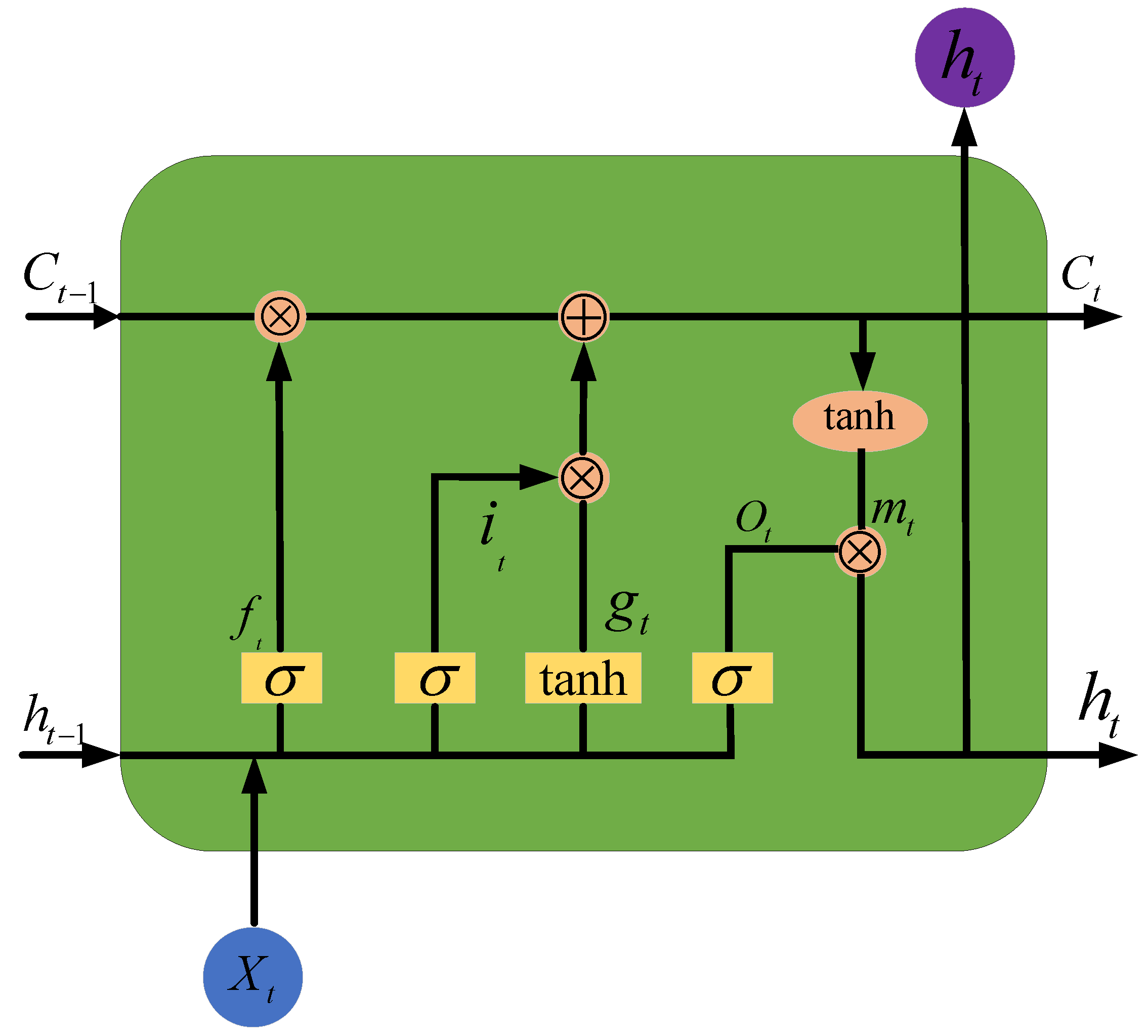
According to the basic principle of LSTM in Section 2, the neural network based on LSTM can be constructed by Equation (20).

$$NE{T}_{LSTM}=\left[X_{real};{\theta }_f,{\theta }_i,{\theta }_g,{\theta }_O;L_{LSTM-\mathrm{loss}}\right]$$

(20)

where ${\theta }_f=\left\{{\omega }_f,b_f\right\}$, ${\theta }_i=\left\{{\omega }_i,b_i\right\}$, ${\theta }_g=\left\{{\omega }_g,b_g\right\}$, ${\theta }_O=\left\{{\omega }_O,b_O\right\}$ stand for the parameters of the forget gate, input gate, input candidate information, and output gate, respectively. $L_{LSTM-\mathrm{loss}}$ represents loss function, which is the same as Equation (12). We optimize the Softmax classifier by minimizing the cost function of Equation (21).

$$L_{LSTM-\mathrm{loss}}=-\frac{1}{t}[\sum _{i=1}^t\sum _{j=1}^N\left\{Label\left(N\right)\right\}·log\frac{{\mathrm{e}}^{h_j}}{{\displaystyle \sum _{l=1}^t}{e}^{{}_{h_l}}}]$$

(21)

where t is the number of states.

3.3. Loss Function Description

For traditional GAN, it is only necessary to optimize the generator by minimizing the cross-entropy loss function shown in Equation (22) and try to make the generated samples consistent with the original sample distribution.

$$L_g=-\frac{1}{k}\sum _{\mathrm{i}=1}^{k}logD{\left(x\right)}_i$$

(22)

To generate more qualified fault samples for fault diagnosis classification, this paper optimizes the training of the generator based on the fault diagnosis results of LSTM and the reconstruction error between $X_{feature-real}$ and ${\widehat{X}}_{feature-real}$. Therefore, the parameters of the generator are optimized by the new loss function defined by the minimization Equation (23) to ensure that the generated samples can be consistent with the original sample distribution and meet the requirements of fault diagnosis.

$$\begin{array}{c}\hfill \begin{array}{c}{L}_{g\_new}=L_g+J_{loss}+L_{LSTM-loss}\hfill \\ =-\frac{1}{k}{\displaystyle \sum _{i=1}^k}logD\left(x\right)\hfill \\ +\frac{1}{J}{\displaystyle \sum _{J=1}^J}{∥X_{feature-real}-X_{feature-fake}∥}_2^2+L_{LSTM-loss}\hfill \end{array}\end{array}$$

(23)

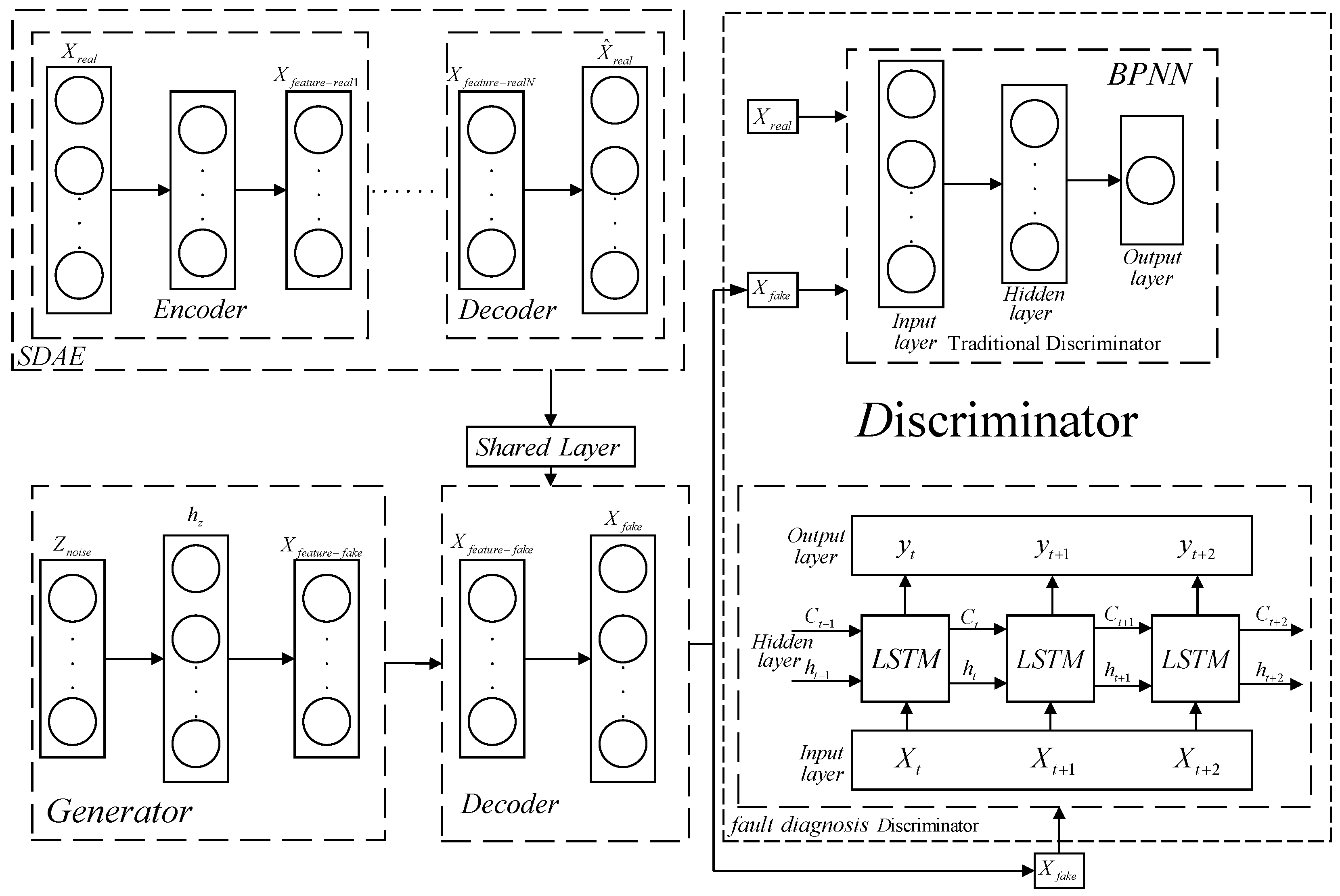
where k is the number of samples, J is the number of deep features extracted from SDAE. The SDAE-GAN-LSTM network structure is shown in Figure 4.

Figure 4. The structure of the SDAE-GAN-LSTM network.

3.4. Diagnosis Process Based on SDAE-GAN-LSTM

The specific iteration steps are as follows:

Step 1

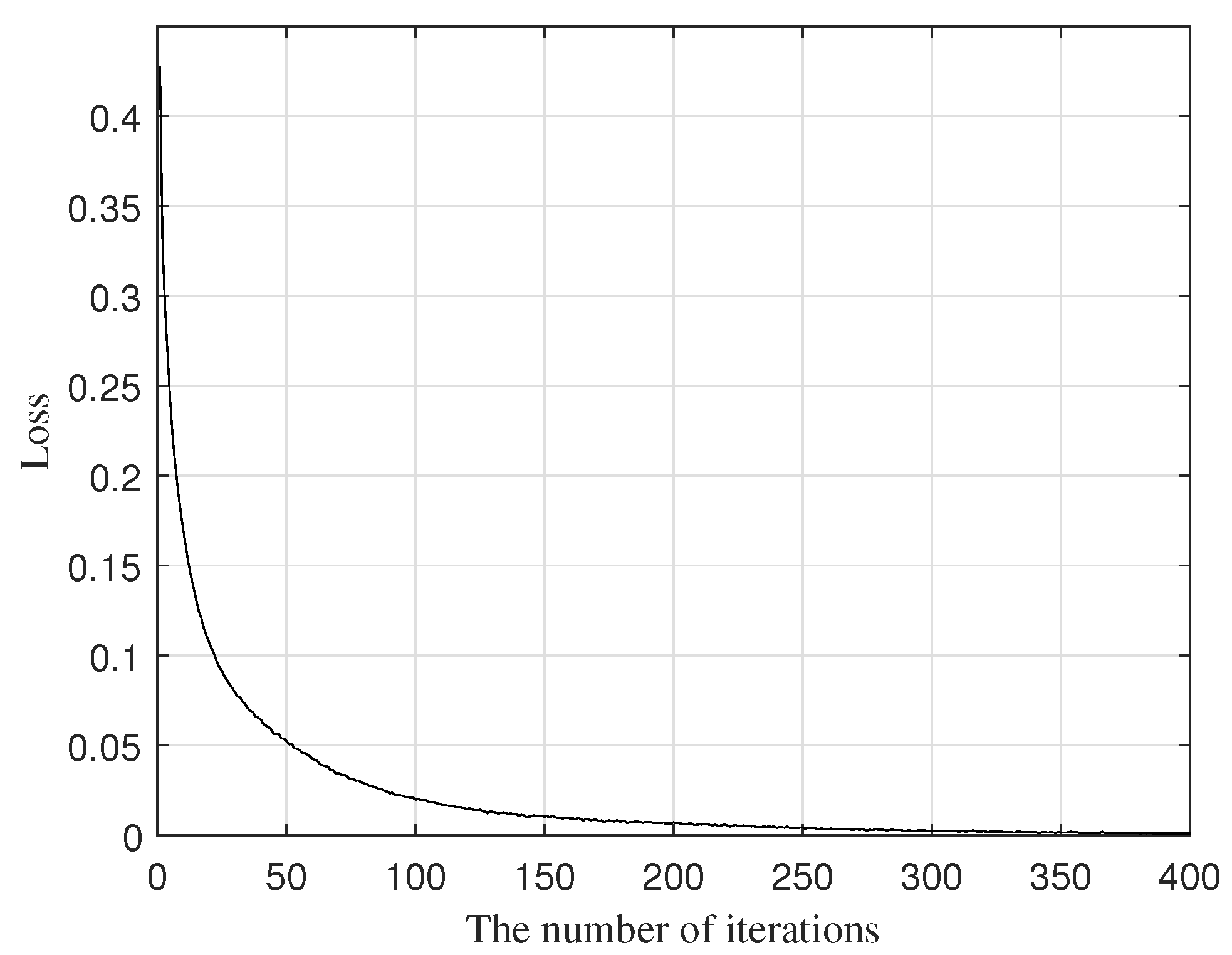
Pre-train the stacked denoising autoencoder.

Given the original fault sample $X_{real}$ as the input, the optimal decoder network can be obtained by following Step 1 to Step 3 in Section 3.1.

Step 2:

Expand the fault sample dataset.

According to Equation (14), the fault features $X_{feature-fake}$ are obtained, and the fault features are decoded by Equation (17) to obtain a new fault sample dataset. Details are shown in Equation (24):

$$X_{data}=\left[X_{real},X_{fake}\right]$$

(24)

Step 3:

Train the traditional discriminator.

Taking $X_{data}$ as the input of the traditional discriminator, the parameters of the discriminator are optimized by minimizing Equation (19).

Step 4:

Pre-train the LSTM-based fault diagnosis discriminator.

Using $X_{data}$ as the input, the fault diagnosis discriminator based on LSTM is trained. In addition, the parameters of Equation (20) are optimized by minimizing Equation (21) to improve the fault identification capability.

Step 5:

Optimize the generator.

$L_d$ and $L_{LSTM-\mathrm{loss}}$ are obtained by optimizing the two discriminators through the generated sample $X_{fake}$ and original fault sample $X_{real}$. We use Equation (23) to optimize the parameters of the generator.

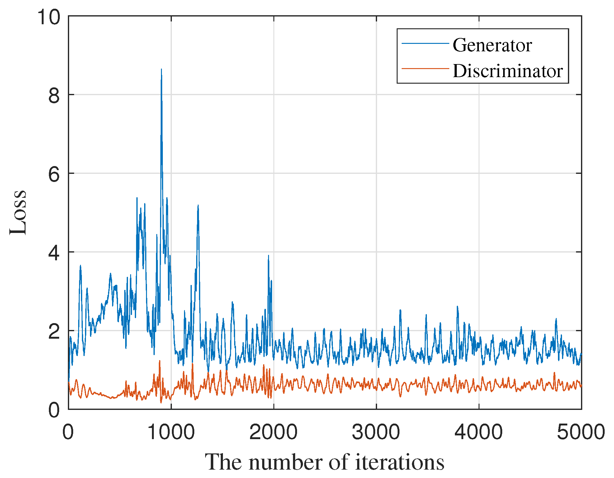
After several iterations, repeat Step 1–Step 5. Record the generator and discriminator loss functions for each iteration. This indicates that the training converges when the Nash equilibrium is reached. Meanwhile, the generator can generate fake samples that are consistent with the distribution of real fault samples to achieve the effect of false confusion. At the same time, the generated samples can achieve high accuracy fault identification requirements based on the LSTM fault diagnosis discriminator.

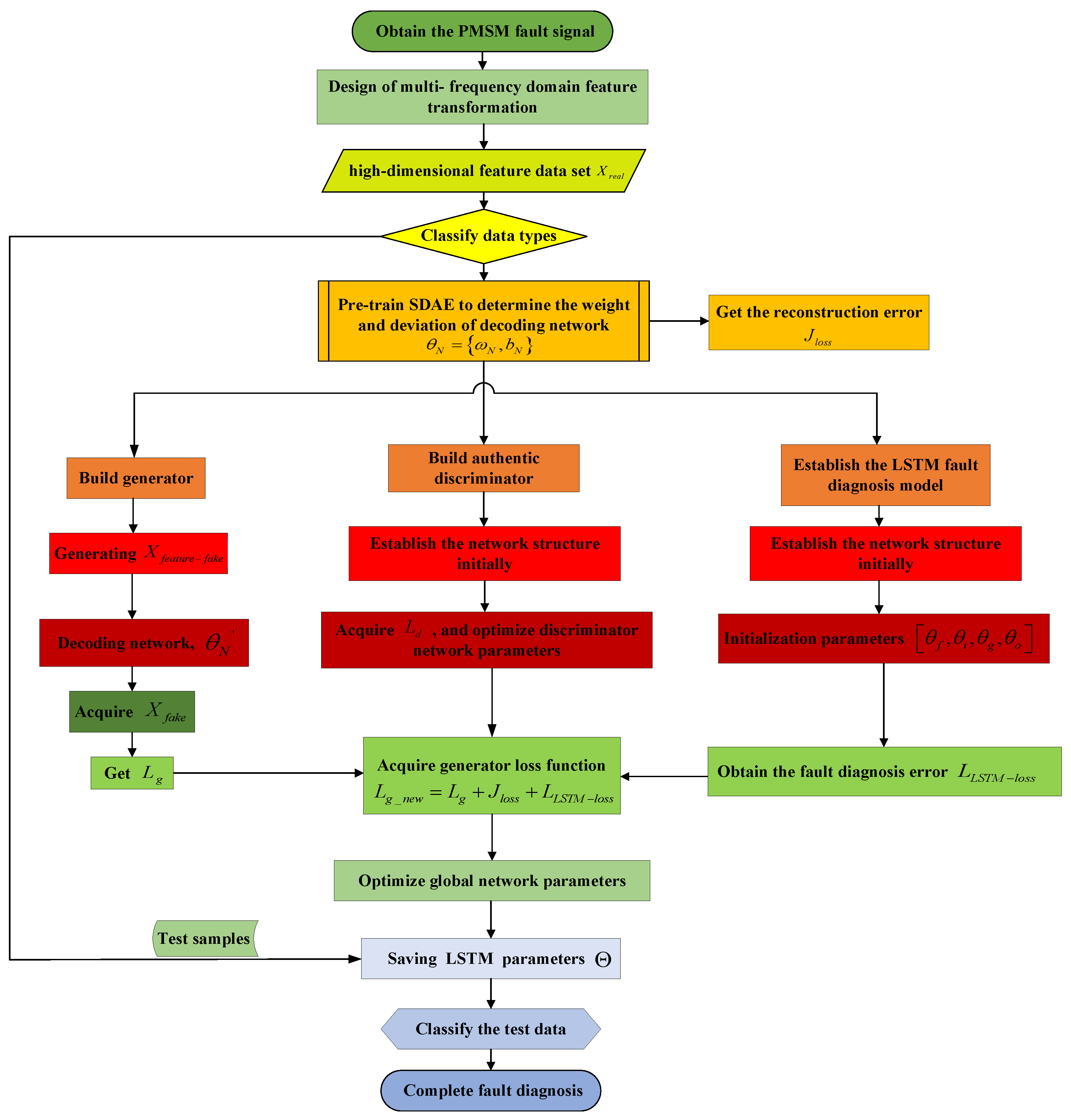
The flow chart of the fault diagnosis algorithm based on SDAE-GAN-LSTM is shown in Figure 5.

Figure 5. Flow chart of fault diagnosis.

4. Simulation Results and Analysis

In this section, the effectiveness of the proposed method is verified by comparing SDAE-GAN-LSTM with typical fault diagnosis methods. The specific experimental analysis will be introduced in detail in this section.

4.1. Experiment

Based on the study of single-bridge arm faults and double-bridge arm faults with a high frequency of inverter open-circuit faults, the fault types can be roughly divided into the following four types:

• Open-circuit fault occurs in the single-bridge arm of the single phase;
• Open-circuit fault occurs in the same side bridge arm of the double phase;
• Open-circuit fault occurs in the double-bridge arm of the single phase;
• Open-circuit fault occurs in the cross-side bridge arm of the double phase.

Based on the study of the inverter phase current’s short-circuit fault, the types of short-circuit faults can be roughly divided into the following three categories:

• Single-phase short circuit;
• Two-phase short circuit;
• Three-phase short circuit.

Next, the above types of open-circuit faults and short-circuit faults are simulated. In the experiment, the pulse signal control strategy is used to control the switch of the IGBT, which can realize the open-circuit fault. Experimental validations were conducted on a three-phase PMSM, with the parameters listed in Table 1 to verify the effectiveness of the proposed method. The block diagram of the three-phase permanent-magnet synchronous motor drive system is shown in Figure 6. And the topology of the three-phase voltage source inverter is shown in Figure 7. In Figure 7, A, B and C represent three-phase bridge arms.

Table 1. Main device parameters.

Items	Specifications
DC Voltage $U_{\mathrm{dc}}$ (V)	311
DC capacitance (mF)	2
Phase resistance R ($\Omega$)	2.875
Phase inductance L (H)	0.0085
Output current frequency (Hz)	60
Output current amplitude (A)	10

Figure 6. The block diagram of the three-phase permanent-magnet synchronous motor drive.

Figure 7. Topology of the three-phase voltage source inverter.

Part of the experiment has high voltage parameters and large current parameters, so it is dangerous to verify the validity of the fault diagnosis method by physical verification. Thus, the MATLAB/Simulink simulation experiment platform was used to verify the effectiveness of this method. The parameters used in the experiment are shown in Table 1. The experimental platform has high precision and can be used as the software simulation environment to verify the fault diagnosis method in this paper.

4.2. Dataset Description

Based on Section 4.1, in the open-circuit fault experiment, the analog current signals are continuously intercepted in one cycle. In the parameter settings, the sampling frequency is 1000 Hz, and the motor load is 0 horsepower. In the simulation, 960 sampling points of three-phase current signals are intercepted in each fault working state. The three-phase current signal under each fault operating state is transformed by the fast Fourier transform, the Short-time Fourier transform, the Gabor transform, the wavelet transform, the Empirical mode decomposition, and the linear canonical transform, respectively. Thus, 3 × 6 groups of feature vectors are obtained for each fault signal to form a multi-feature dataset, and each group has 480 sampling points. Then, under the premise that the feature structure is relatively unchanged, in order to reduce the calculation errors caused by data differences, the max–min normalization method shown in Equation (25) is used to normalize all sets of feature data to the range of [0, 1]. In the simulation, there are 480 × 5 sampling points of data in 5 working conditions, which includes 4 fault working conditions and 1 fault-free working condition. After the samples are scrambled, 50% of the data samples are randomly selected as the training set, and the remaining 50% of the data samples are selected as the test set. The three-phase stator current fault data are described in Table 2.

$$x^{*}=\frac{x-x_{min}}{x_{max}-x_{min}}$$

(25)

Table 2. Description of the three-phase stator current fault data.

Faulty Type	Number of Samples	Tag
Fault-free	480	T1
The single-bridge arm of the single phase	480	T2
The same-side bridge arm of the double phase	480	T3
The double-bridge arm of the single phase	480	T4
The cross-side bridge arm of the double phase	480	T5

4.3. Detailed Structure and Parameter Selection of SDAE-GAN-LSTM

We created the network model structure shown in Figure 4. In the experiment, according to the steps in Section 3.1, the original fault samples were used for pre-training SDAE to obtain the optimal decoding network. In order to obtain the result of the global optimal fault diagnosis, the optimal hyperparameters of the program were obtained through several iterative simulation experiments. The reconstruction error of the SDAE training is shown in Figure 8. As seen in Figure 8, with the increase in iterations, the training error began to decrease, showing a trend of convergence.

Figure 8. Change of SDAE loss.

From the perspective of improving the efficiency of the model and reducing the repetitive training of the model, this paper uses the characteristics of transfer learning to migrate the optimized decoder network into the generator to decode $X_{feature-fake}$, and constantly optimize the improved GANs until Nash equilibrium is reached. The unbalanced samples are classified based on the LSTM network. Finally, the imbalance sample fault diagnosis classification is performed based on the LSTM network. The parameters of the SDAE-GAN-LSTM optimal network model established in this part of the simulation test are shown in Table 3.

Table 3. The optimal detailed structures and parameters of SDAE-GAN-LSTM.

Training Parameter	Pre-Training Model	Generator	Discriminator	Fault Diagnosis Model
Number of layers	5	4	3	3
Number of neurons on each layer	18/50/30/18/5	18/50/30/18	18/50/1	18/30/5
Learning rate	0.1	0.01	0.01	auto
Bach size	6	480	480	20
Maximum of iteration times	400	5000	5000	100
The denoising	0.5	/	/	/
Optimizer	/	Adam	Adam	Adam
		Leaky relu	Leaky relu	Sigmoid
Activation function on each layer	Sigmoid	Leaky relu	Sigmoid	Tanh
		Sigmoid

4.4. Analysis of Results

In order to avoid the contingency of simulation experiments, this paper conducts 10 repeated simulations and takes the one with the highest accuracy as an example. The generative adversarial network continuously updates the gradient according to the improved loss function equation, i.e., Equation (23). The generator’s network parameters and the discriminator’s network parameters are gradually optimized so that the generator generates discriminative fault data samples that are closer to reality. The generator loss and discriminator loss are obtained after 5000 iterations, as shown in Figure 9. It can be seen from Figure 9 that the generator and discriminator achieve Nash equilibrium. In this case, the distribution of the generated samples is similar to that of the actual samples, which can be used as input for fault diagnosis.

Figure 9. Change of GAN loss.

In this simulation experiment, each group has 480 sampling points of training data. To reduce the impact of randomness, 1000 sets of generated samples are produced by the generator for each group, resulting in a total of 1480 data sampling points within each group. This aggregation yields five categories, amounting to a combined dataset of 7400 sampling points. To ensure the generalization of the method, 50% of the data samples are randomly selected as the training set, and the remaining 50% of the data samples are used as the test set.

The parameters of the simulation experiment are as shown in Table 4; the LSTM neural network hidden layer neurons are 30. The maximum number of training iterations is 100 and the batch size is set to 20. The optimizer used is Adam. The gradient threshold is set to 1. After setting the simulation parameters, the simulation verification is carried out. The actual classification diagram and predictive classification diagram of the five fault types are shown in Figure 10. The red dots represent the predicted classification results, and the blue circles represent the actual classification results. The coincidence of red dots and blue circles indicates that the fault diagnosis result is correct. Otherwise, the diagnosis is incorrect.

Table 4. Network model parameters of a typical fault diagnosis model.

Method	Pre-Training Model	Generator	Discriminator	Fault Diagnosis Model
SAE	Number of layers	/	/	5
	Number of neurons on each layer	/	/	18/50/30/18/5
	Learning rate	/	/	0.1
	Maximum of iteration times	/	/	400
GAN-SAE	Number of layers	4	3	5
	Number of neurons on each layer	18/50/30/18	18/50/1	18/50/30/18/5
	Learning rate	0.01	0.01	0.1
	Maximum of iteration times	5000	5000	200
LSTM	Number of layers	/	/	3
	Number of neurons on each layer	/	/	18/30/5
	Learning rate	/	/	Auto
	Maximum of iteration times	/	/	200
GAN- LSTM	Number of layers	4	3	3
	Number of neurons on each layer	18/50/30/18	18/50/1	18/30/5
	Learning rate	0.01	0.01	Auto
	Maximum of iteration times	5000	5000	100
BPNN	Number of layers	/	/	3
	Number of neurons on each layer	/	/	18/100/5
	Learning rate	/	/	0.1
	Maximum of iteration times	/	/	300

Figure 10. The fault classification result diagram of SDAE-GAN-LSTM under the open-circuit fault.

It is concluded from Figure 10 that the accuracy of the proposed method in the multi-classification is as high as 98.919%, which proves that the method can effectively complete the fault diagnosis classification. From the classification results, the proposed method is assisted due to the multi-dimensional fault features, making the proposed model achieve a better classification effect.

Figure 11 clearly shows the confusion matrix of SDAE-GAN-LSTM (using the highest accuracy as an example). It should be noted that the columns represent the actual classifications and the rows represent the predicted classifications. It can be concluded from the diagram that the main error comes from the fifth fault category. Meanwhile, Table 5 reveals the F-measure and sensitivity of the proposed method in multi-classification, which demonstrates that the method has a good classification effect.

Figure 11. Confusion matrix of SDAE-GAN-LSTM under the open-circuit fault.

Table 5. Classification evaluation index.

Name	Tag1	Tag2	Tag3	Tag4	Tag5	macroAVG
sensitivity	100%	99.01%	99.19%	98.80%	97.60%	98.92%
F-measure	99.86%	98.32%	99.39%	99.06%	97.93%	98.91%

In the experiment on short-circuit faults, three types of short-circuit faults are classified and identified by the proposed method. The parameters of the simulation experiment are the same as those of the open-circuit fault experiment. It can be concluded from Figure 12 that in the case of short-circuit faults, the method proposed in this paper also plays a good role in the classification and identification of fault diagnosis, with an accuracy rate of 99.96%. As seen in Figure 13, there is only one sample discrimination error, which proves the effectiveness of this method in data-driven engineering fault diagnosis.

Figure 12. The fault classification result diagram of SDAE-GAN-LSTM under the short-circuit fault.

Figure 13. Confusion matrix of SDAE-GAN-LSTM under the short-circuit fault.

4.5. Comparison between Fault Diagnosis Results under Different Transformations

To verify that a multi-feature dataset can improve the accuracy of fault identification by the diagnosis model, the proposed multi-feature fusion method in this paper is used for fault diagnosis in comparison with the single feature dataset. To avoid contingencies, based on the SDAE-GAN-LSTM model, this paper conducted 10 repeated experiments to obtain the average accuracy, maximum accuracy, and standard deviation of different feature datasets. The comparison of results is shown in Figure 14. As can be seen from Table 6, the multi-feature dataset has a significant improvement, which is better than the fault diagnosis recognition rate under a single feature dataset. Furthermore, the standard deviation of the diagnosis result of the multi-feature is smaller, which proves that the model stability is higher. According to the classification results, the multi-feature dataset enhances the classification effect, which verifies the effectiveness of the multi-feature fusion method.

Figure 14. Fault diagnosis accuracy for different transformations.

Table 6. Fault identification accuracy under different transformations.

Feature Transform Method	Mean Diagnostic Accuracy	Maximum Diagnostic Accuracy	Standard Deviation
FFT	53.73%	76.78%	0.2028
STFT	52.14%	67.84%	0.0681
Gabor	30.28%	33.95%	0.0796
Wavelet	84.23%	87.81%	0.0163
EMD	84.19%	85.73%	0.0119
Linear transformation	79.93%	85.05%	0.0719
Multi-feature fusion	98.63%	98.92%	0.0036

4.6. Comparison with Typical Fault Diagnosis

In order to evaluate the superiority of the proposed method, this paper compares SDAE-GAN-LSTM with five typical fault diagnosis methods, including SAE, GAN-SAE, GAN-LSTM, LSTM, and back propagation neural network (BPNN). The network model parameters established by simulation are shown in Table 4.

The mean diagnostic accuracy, maximum diagnostic accuracy, and standard deviation of each diagnostic method are calculated. The simulation results are recorded in Table 7. The smaller the standard deviation, the more stable the result is. Figure 15 shows the fault diagnosis accuracy curves of SAE, GAN-SAE, LSTM, GAN-LSTM, BPNN, and SDAE-GAN-LSTM, respectively.

Table 7. Fault recognition accuracy under different models.

Fault Diagnostic Models	Mean Diagnostic Accuracy	Maximum Diagnostic Accuracy	Standard Deviation
SAE	92.70%	94.83%	0.0129
GAN-SAE	90.18%	91.18%	0.0094
LSTM	91.10%	93.25%	0.0123
GAN- LSTM	93.96%	94.68%	0.0043
BPNN	92.40%	94.79%	0.0143
SDAE-GAN-LSTM	98.63%	98.92%	0.0036

Figure 15. Diagnostic accuracies of the 10 trials.

After repeated simulations, the SDAE-GAN-LSTM method has demonstrated remarkable accuracy in fault diagnosis. It can be seen from Table 7 and Figure 15 that the SDAE-GAN-LSTM not only exhibits the smallest standard deviation but also showcases the narrowest fluctuation range among the six methods under consideration. In reference [33], the authors employed stacked autoencoders (SAE) to compress the original data for gear pitting fault diagnosis, highlighting the effectiveness of the proposed SDAE-GAN-LSTM method in comparison. Furthermore, reference [34] proposed a fault diagnosis method, GAN-SAE, to address data imbalance issues, particularly in diagnosing electric feed pump faults. This approach significantly improved fault diagnosis accuracy, serving as a foundation for evaluating the effectiveness of the SDAE-GAN-LSTM method across diverse applications. In the context of time series data, reference [35] introduced an enhanced model structure tailored toward tackling sample imbalance problems. This method, employing LSTM as the classifier, achieved progressively higher accuracy as the number of fault samples increased. Additionally, the incorporation of GAN further bolstered the model’s resistance to noise. Notably, this approach exhibited excellent performance in diagnosing faults in three-phase PMSM drive system inverters, leading to improved classification and recognition accuracy. Comparative tests conducted in references [34,35], involving various algorithms, revealed that the proposed SDAE-GAN-LSTM method consistently produced experimental results either comparable to or superior to existing methods. This substantiates the superiority and effectiveness of the SDAE-GAN-LSTM approach in fault diagnosis. For a concise summary, please refer to Table 8, which presents a comprehensive comparison between the methods discussed in the current literature and those proposed in this paper. This comparison unequivocally demonstrates that the proposed SDAE-GAN-LSTM method outperforms others in terms of fault diagnosis accuracy and provides stable diagnosis results.

Table 8. Comparison between the methods in this paper and those in the current literature.

Fault Diagnostic Models	Diagnostic Accuracy	Application Object
SAE in [33]	93.46%	Gear pitting
GAN-SAE in [34]	98.89%	Electrically driven feed pump
GAN- LSTM in [35]	69.67%	Aircraft
SDAE-GAN-LSTM	98.92%	PMSM

5. Conclusions

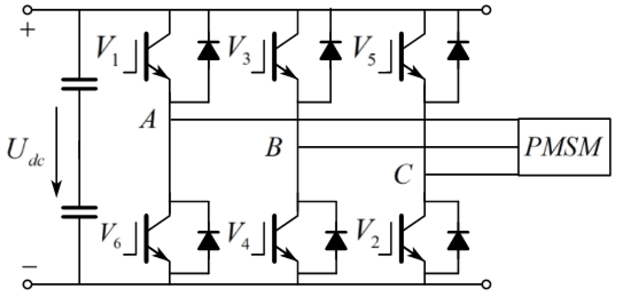
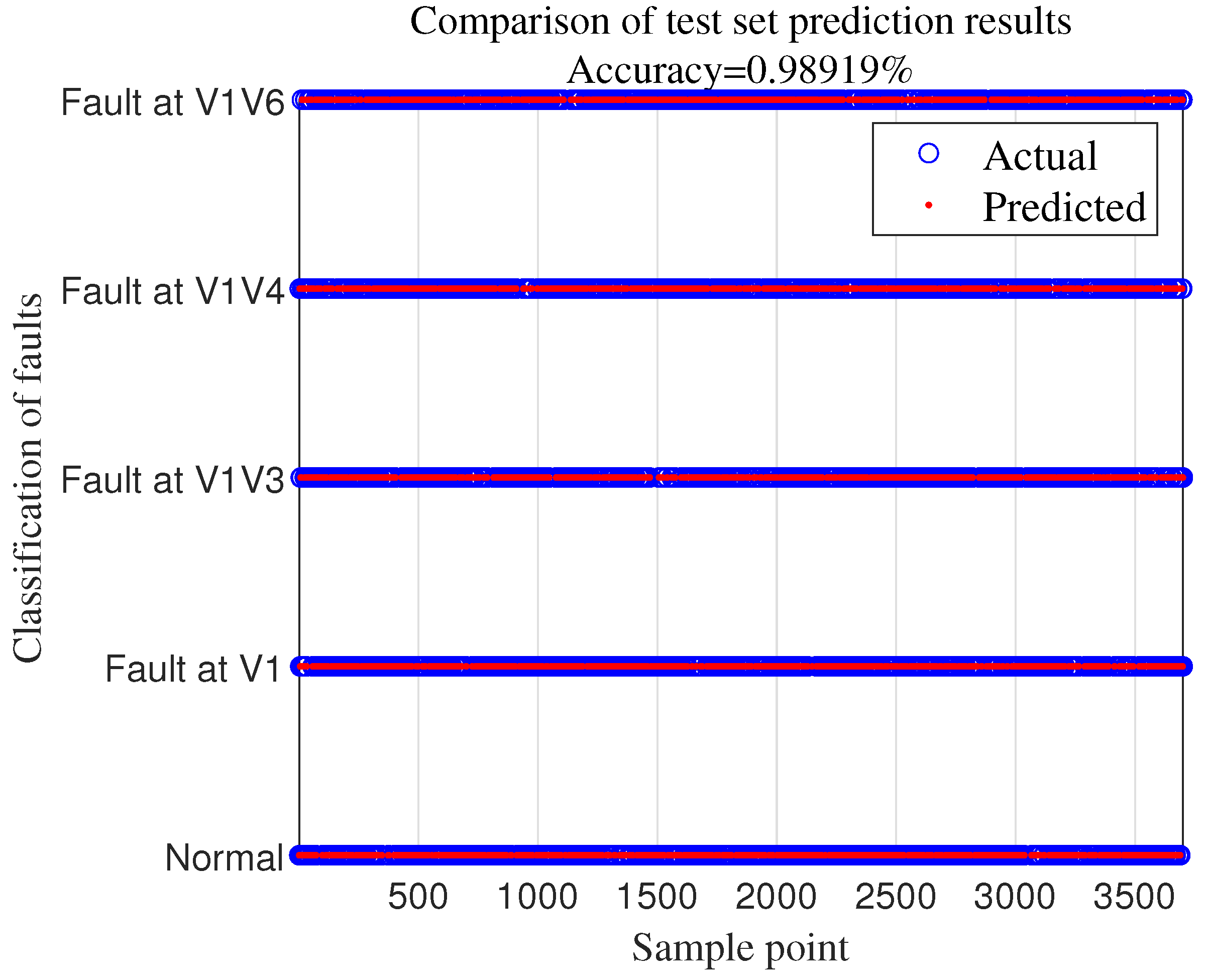
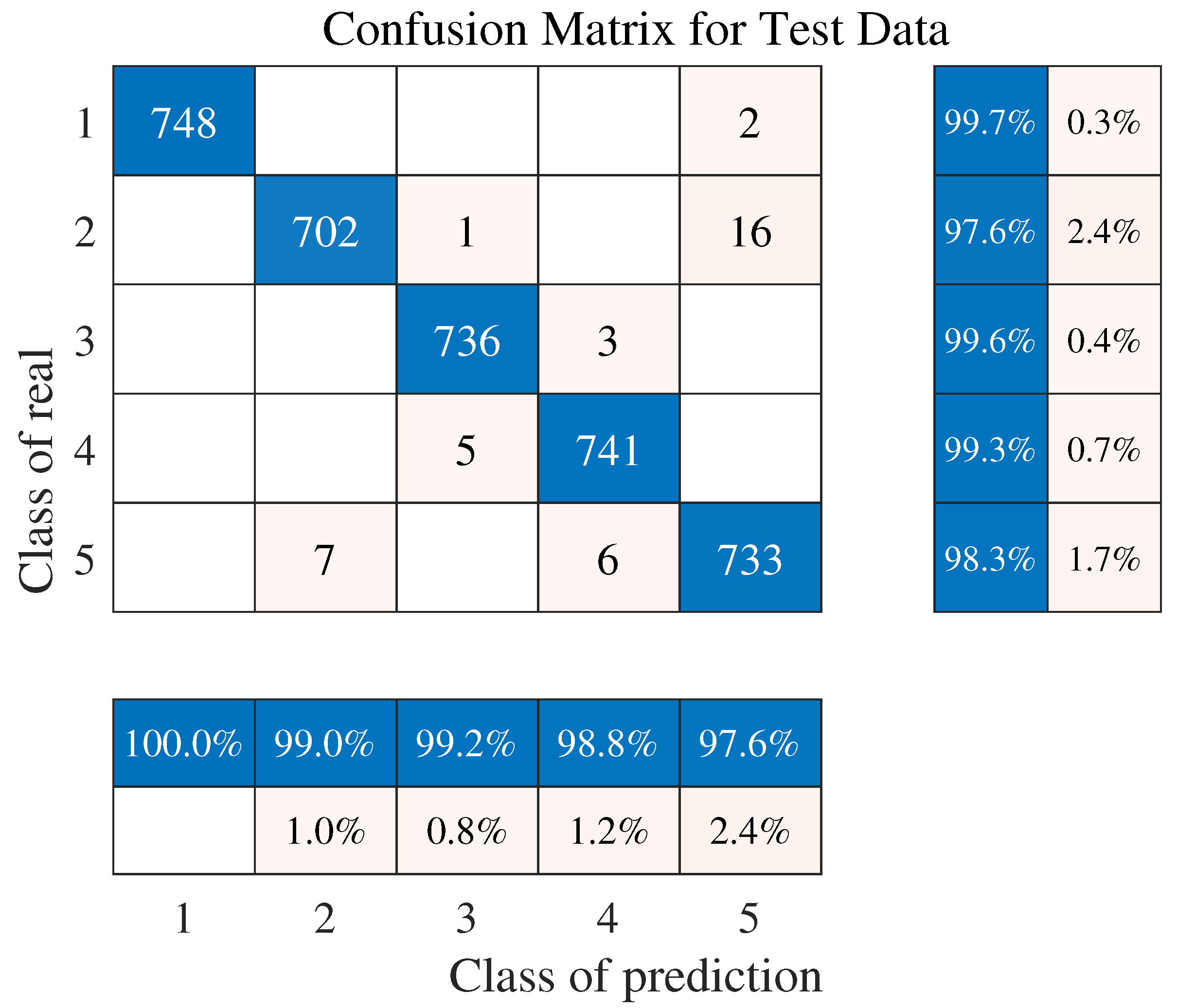
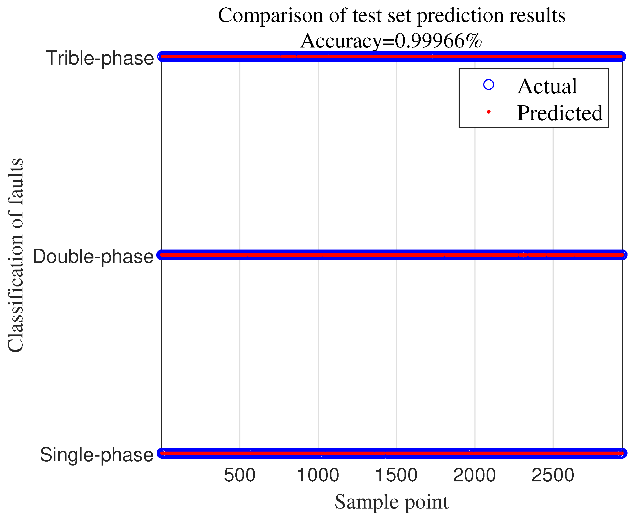
An improved fault diagnosis method is proposed, which can diagnose the open-circuit fault and short-circuit fault of the inverter in a three-phase permanent-magnet synchronous motor drive system. The main advantages of this method are as follows. First, the pre-trained SDAE network decodes the fake features, enhancing the model’s robustness, and ensuring that the generated samples meet the requirements of fault identification. Secondly, leveraging the potent sample generation capabilities and data feature extraction ability of the GANs, high-quality samples with similar distributions—satisfying fault discrimination—are generated. Finally, the adaptive learning capabilities of the LSTM network in processing time series data are leveraged to further integrate feature information and predict fault diagnosis outcomes. Through a series of comparative experiments on open-circuit fault diagnosis in the inverter of a three-phase PMSM drive system, the classification accuracy of the proposed method can reach 98.92%, which shows the effectiveness of the proposed method. Furthermore, for inverter short-circuit faults in the three-phase permanent-magnet synchronous motor drive system, the classification and identification accuracy reaches an impressive 99.96%. In contrast, the accuracies of SAE, GAN-SAE, LSTM, GAN-LSTM, and BPNN are 94.83%, 91.18%, 93.25%, 94.68%, and 94.79%, respectively. Consequently, this method holds significant reference value for open-circuit fault and short-circuit fault diagnosis in three-phase permanent-magnet synchronous motor drive systems.

It is important to acknowledge that the above research comes with certain limitations. The fault experiment of the permanent-magnet synchronous motor drive system was completed in a very ideal state in the simulation software while ignoring the influence of external objective factors, such as temperature and load on the motor work. In light of these limitations, future research endeavors will aim to address these gaps. Specifically, in future research, we intend to investigate the operation and failure modes of the permanent-magnet synchronous motor drive system in more complex and realistic environments. This will involve conducting experiments that account for the influence of temperature fluctuations and varying loads on motor performance, providing a more comprehensive understanding of system behavior. Additionally, in terms of algorithmic advancements, we plan to delve deeper into the problem of adaptive optimization in future work. This will involve exploring and developing algorithms that can further enhance the adaptability and performance of our proposed method in diverse operational scenarios. In future research, efforts should be made to continuously improve the experimental procedure to improve the generalization and robustness of the method and ensure its applicability in the actual environment. In conclusion, while this study has produced promising results, this paper acknowledges that further exploration and refinement are needed to make the proposed method more resilient and adaptable in practical applications.

References

1. Delpoux, R.; Hetel, L.; Kruszewski, A. Parameter-dependent relay control: Application to PMSM. IEEE Trans. Control. Syst. Technol. 2014, 23, 1628–1637. [Google Scholar] [CrossRef]
2. Zhang, Q.; Yu, R.; Li, C.; Chen, Y.; Gu, J. Servo Robust Control of Uncertain Mechanical Systems: Application in a Compressor/PMSM System. Actuators 2022, 11, 42. [Google Scholar] [CrossRef]
3. Lei, Y.; Li, N.; Guo, L.; Li, N.; Yan, T.; Lin, J. Machinery health prognostics: A systematic review from data acquisition to RUL prediction. Mech. Syst. Signal Process. 2018, 104, 799–834. [Google Scholar]
4. Wang, T.; Liu, L.; Zhang, J.; Schaeffer, E.; Wang, Y. M-EKF fault detection strategy of insulation system for marine current turbine. Mech. Syst. Signal Process 2019, 115, 269–280. [Google Scholar] [CrossRef]
5. Zhou, F.N.; Wen, C.L.; Leng, Y.B.; Chen, Z.G. A data-driven fault propagation analysis method. Chem. Ind. Eng. China 2010, 61, 1993–2001. [Google Scholar]
6. Wang, T.; Wu, H.; Ni, M.; Zhang, M.; Dong, J.; Benbouzid, M.E.H.; Hu, X. An adaptive confidence limit for periodic non-steady conditions fault detection. Mech. Syst. Signal Process 2016, 72, 328–345. [Google Scholar] [CrossRef]
7. Priyadharshini, P.; Archana, M.V.; Elsayed, E.M.; Vivek, D. A Model for an Application to Biomedical industry through Viscoinelastic nanofluid flow. Mach. Learn. 2023, 2, 10–19. [Google Scholar]
8. Guan, H.; Hao, G.; Yan, Z. A novel fault diagnosis method for smart grid based on data drive theory. Adv. Sci. Technol. Lett. 2014, 73, 67–74. [Google Scholar]
9. Wang, T.; Zhang, L.; Wang, X. Fault detection for motor drive control system of industrial robots using CNN-LSTM-based observers. CES Trans. Electr. Mach. Syst. 2023, 7, 23389105. [Google Scholar] [CrossRef]
10. Mao, Y.; Zheng, M.; Wang, T.; Duan, M. A new mooring failure detection approach based on hybrid LSTM-SVM model for semi-submersible platform. Ocean Eng. 2023, 275, 114161. [Google Scholar] [CrossRef]
11. Sun, Z.; Machlev, R.; Wang, Q.; Belikov, J.; Levron, Y.; Dmitry, B. A public data-set for synchronous motor electrical faults diagnosis with CNN and LSTM reference classifiers. Energy AI 2023, 14, 100274. [Google Scholar] [CrossRef]
12. Zhao, H.; Sun, S.; Jin, B. Sequential fault diagnosis based on LSTM neural network. IEEE Access 2018, 6, 12929–12939. [Google Scholar] [CrossRef]
13. Mohammad-Alikhani, A.; Nahid-Mobarakeh, B.; Hsieh, M.F. One-Dimensional LSTM-Regulated Deep Residual Network for Data-Driven Fault Detection in Electric Machines. IEEE Trans. Ind. Electron. 2023, 71, 3083–3092. [Google Scholar] [CrossRef]
14. Xue, Z.Y.; Xiahou, K.S.; Li, M.S.; Ji, T.Y.; Wu, Q.H. Diagnosis of multiple open-circuit switch faults based on long short-term memory network for DFIG-based wind turbine systems. IEEE J. Emerg. Sel. Top. Power Electron. 2019, 8, 2600–2610. [Google Scholar] [CrossRef]
15. Zou, P.; Hou, B.; Lei, J.; Zhang, Z. Bearing fault diagnosis method based on EEMD and LSTM. Int. J. Comput. Commun. Control. 2020, 15. [Google Scholar] [CrossRef]
16. Goodfellow, I.; Pouget-Abadie, J.; Mirza, M.; Xu, B.; David, W.F.; Sherjil, O.; Aaron, C.; Yoshua, B. Generative Adversarial Nets in Advances in Neural Information Processing Systems (NIPS); Curran Associates, Inc.: Red Hook, NY, USA, 2014; Volume 10, pp. 2672–2680. [Google Scholar]
17. Carrasco, X.A.; Elnagar, A.; Lataifeh, M. A Generative Adversarial Network for Data Augmentation: The Case of Arabic Regional Dialects. Procedia Comput. Sci. 2021, 189, 92–99. [Google Scholar] [CrossRef]
18. Chen, B. A Research on Fault Diagnosis of Wind Turbine CMS Based on Bayesian-GAN-LSTM Neural Network. J. Phys. Conf. Ser. IOP Publ. 2022, 2417, 012031. [Google Scholar]
19. Shi, J.; Ding, Y.; Lv, Z. An intermittent fault data generation method based on lstm and gan. In Proceedings of the 2021 Global Reliability and Prognostics and Health Management (PHM-Nanjing), Nanjing, China, 15–17 October 2021; pp. 1–4. [Google Scholar]
20. Lu, S.; Ding, Y.; Liu, M.; Yin, Z.; Yin, L.; Zheng, W. Multiscale feature extraction and fusion of image and text in VQA. Int. J. Comput. Intell. Syst. 2023, 16, 54. [Google Scholar]
21. Ma, P.; Ren, J.; Sun, G.; Zhao, H. Multiscale superpixelwise prophet model for noise-robust feature extraction in hyperspectral images. IEEE Trans. Geosci. Remote Sens. 2023, 61, 1–12. [Google Scholar] [CrossRef]
22. Wu, P.; Wang, Z.; Zheng, B.; Li, H.; Alsaadi, F.E.; Zeng, N. AGGN: Attention-based glioma grading network with multi-scale feature extraction and multi-modal information fusion. Comput. Biol. Med. 2023, 152, 106457. [Google Scholar]
23. Xie, J.; Li, Z.; Zhou, Z.; Liu, S. A novel bearing fault classification method based on XGBoost: The fusion of deep learning-based features and empirical features. IEEE Trans. Instrum. Meas. 2020, 70, 1–9. [Google Scholar] [CrossRef]
24. Jia, F.; Lei, Y.; Lin, J.; Zhou, X.; Lu, N. Deep neural networks: A promising tool for fault characteristic mining and intelligent diagnosis of rotating machinery with massive data. Mech. Syst. Signal Process. 2016, 72, 303–315. [Google Scholar]
25. Bin, G.F.; Gao, J.J.; Li, X.J.; Dhillon, B.S. Early fault diagnosis of rotating machinery based on wavelet packets—Empirical mode decomposition feature extraction and neural network. Mech. Syst. Signal Process. 2012, 27, 696–711. [Google Scholar] [CrossRef]
26. Fei, S. Fault diagnosis of bearing based on wavelet packet transform-phase space reconstruction-singular value decomposition and SVM classifier. Arab. J. Sci. Eng. 2017, 42, 1967–1975. [Google Scholar] [CrossRef]
27. Liu, H.; Zhao, H.; Wang, J.; Yuan, S.; Feng, W. LSTM-GAN-AE: A promising approach for fault diagnosis in machine health monitoring. IEEE Trans. Instrum. Meas. 2021, 71, 1–13. [Google Scholar] [CrossRef]
28. Vincent, P.; Larochelle, H.; Bengio, Y.; Manzagol, P.A. Extracting and composing robust features with denoising autoencoders. In Proceedings of the 25th International Conference on Machine Learning, Helsinki, Finland, 5–9 July 2008; pp. 1096–1103. [Google Scholar]
29. Du, X.; Jia, L.; Haq, I.U. Fault diagnosis based on SPBO-SDAE and transformer neural network for rotating machinery. Measurement 2022, 188, 110545. [Google Scholar]
30. Fu, Q.; Wang, H. A novel deep learning system with data augmentation for machine fault diagnosis from vibration signals. Appl. Sci. 2020, 10, 5765. [Google Scholar] [CrossRef]
31. Chen, Y.; Liu, Y.; Jiang, D.; Zhang, X.; Dai, W.; Xiong, H.; Tian, Q. Sdae: Self-distillated masked autoencoder. In European Conference on Computer Vision; Springer Nature: Cham, Switzerland, 2022; pp. 108–124. [Google Scholar]
32. Greff, K.; Srivastava, R.K.; Koutnik, J.; Steunebrink, B.R.; Schmidhuber, J. LSTM: A Search Space Odyssey. IEEE Trans. Neural Netw. Learn. Syst. 2017, 28, 2222–2232. [Google Scholar] [CrossRef]
33. Li, J.; Li, X.; David, H.; Yangzhi, Q. LSTM: A novel method for early gear pitting fault diagnosis using stacked SAE and GBRBM. Sensors 2010, 19, 758. [Google Scholar] [CrossRef]
34. Han, H.; Hao, L.; Cheng, D.; Xu, H. GAN-SAE based fault diagnosis method for electrically driven feed pumps. PLoS ONE 2020, 15, e0239070. [Google Scholar]
35. Shen, K.; Zhao, D. A Fault Diagnosis Method under Data Imbalance Based on Generative Adversarial Network and Long Short-Term Memory Algorithms for Aircraft Hydraulic System. Aerospace 2023, 10, 164. [Google Scholar] [CrossRef]