Explained Learning and Hyperparameter Optimization of Ensemble Estimator on the Bio-Psycho-Social Features of Children and Adolescents

Abstract

For decades, projects have been carried out in various countries to assess the developmental status of children and adolescents using anthropometry and specific kinesiological measurements. There is a need for the ability to evaluate this developmental status using a sufficiently simple method or a calculation to be applicable in practice. The most commonly used feature for this purpose is currently body mass index (BMI). From recent experience, this feature may cause problems if used indiscriminately in the developmental phase of life. Therefore, we aimed to find a more suitable feature set. We used data from Artos, the national program monitoring school children and adolescents in Slovenia. The data was analyzed using machine learning (ML) tools to find the most important features to predict a motor efficiency index (MEI), which has been shown to correlate strongly with a person’s health prospects. After data preparation and training a baseline model, a feature selection process was performed, which promoted some features as candidates to predict the motor efficiency index sufficiently. By implementing a hyperparameter optimization, we tuned the ML model to improve its generalization and present the feature interaction more elaborately. We show that besides the single feature’s importance, the features’ interaction should be considered. In the case of MEI, we find that the skin fold thicknesses can complement BMI and contribute to a better development status assessment of children and adolescents.

1. Introduction

Several countries have established regular campaigns to examine the growth and development of the young population—children and adolescents. The National Health and Nutrition Examination Survey is performed yearly in the USA, and in Holland, The Amsterdam Growth and Health Longitudinal Study is conducted [1]. In Slovenia, the Faculty of Sport at the University of Ljubljana initiated a pioneering project called Artos in the decade of 1960, which is still ongoing today [2]. The project investigates the interconnection between children’s motor development and their functional capacities and bodily, emotional, mental, and social status dimensions, as well as the impact of the environment. All these features combined define quality of life and health in a broad sense. The measurements consist of assessing various motoric tasks and measurements of body dimensions. Additionally, the participants complete two surveys. All the anthropometry is performed noninvasively; no samples of body liquids or tissues are collected. The lengths, widths, and circumferences of limbs and torso are measured using meters, scales, calipers, and special compasses. These measurements as a whole are termed bio-psycho-social properties. Project Artos has been conducted to the present and continues.

In the scientific literature, most attention among the anthropometric data has been paid to the body mass index (BMI), defined as body mass divided by the square of the body height (kg/m²). Practitioners have simple tools at their disposal to assess the status of an individual in the form of growth charts that are percentile based and drawn from population surveys over many years. However, some doubts about the use of BMI arise because there are still some problems with scientific evidence [3]. In addition to overweight and obesity, thinness also poses health problems [4]. Other indicators have been proposed, e.g., the Slaughter formula [5], which is not ideal either.

Hence, our aim is to:

• Find more conclusive evidence of the role that BMI plays in the healthy development of children and adolescents or to
• Find other features that could substitute or amend it.

The method presented in this study used to find such features among the collected data is feature selection, specifically the greedy feature selection (GFS) method [6]. This method selects the most important feature first and then adds other features that improve prediction the most. The research question is about which features influence the motor efficiency index (MEI) the most, so the GFS is a natural choice for this task.

We then use graphic tools to show the model decisions. Such tools are needed because the selected machine learning method acts like a black box—the model has too many parameters to be easily comprehensible. These tools can help us to better tune model hyperparameters into the desired direction suitable for our goals.

Studies [7,8] show that high blood lipid levels can be linked to both BMI and insufficient physical activity. Studies also show that it is possible to reduce health risks by increasing physical activity. It is shown that children with high BMI and a high level of aerobic effectiveness have a lower risk of metabolic syndrome than those with high BMI and lower aerobic capacity [9]. It has also been shown that the epidemic dimension of obesity can be primarily attributed to physical inactivity rather than excessive caloric intake. As a preventive and corrective measure, it is suggested that persons with high BMI should increase physical activity and, consequently, their fitness, which can improve their health prospects for later life [10]. In this sense, we try to analyze the Artos data and find its relationship with MEI. It is defined as a function of the results of motoric tests according to EUROFIT [11] and SLOfit [12] protocols, which are also part of the Artos data. This index is an indicator of fitness. It serves as the predicted variable, and predictions are made from other features.

In the Experiment section, we present the necessary steps to preprocess the data and the initial machine learning tests. Then, in the Feature Selection and Evaluation section, we present intermediate results. In the Tuning by Optimization section, we develop the process of tuning the model parameters to obtain clearer insights into the data. Additionally, in the Spearman’s Rank Coefficient as a Source of Feature Importance Information section, we present another view of the data through their statistical properties. In the Discussion section, we present the current study’s limitations, compare our work with related publications, and envision possible directions for future work. Finally, in the Conclusions, we summarize the important findings.

2. Materials and Methods

2.1. Data Pre-Processing

We analyzed the Artos data from the last completed measurement campaign from the years 2013 and 2014. The data were obtained in another study following protocol [2] and under the supervision of their original authors; therefore, explicit ethical approval was not needed. The children and adolescents were selected from various primary and secondary schools so that a nationally representative sample was obtained with regard to sex, age, size of city or town, geographical region, and, in the case of secondary schools, program. All further details about the sample are available in the study protocol [2].

The first step in the preparation of the Artos data was to divide the dataset in two groups based on sex. The reason for this division is that the development in the studied age period is different for each sex. The feature set is also different for each sex. All the data preparatory activities were performed separately for each sex.

The motor efficiency index was calculated in three components following the same principle as defined in [13]:

• Neuromuscular Fitness (NMF),
• Muscular Fitness (MF), and
• Cardiorespiratory Fitness (CRF).

Each MEI component is dependent on a subset of the physical performance features. These features were discretized by centiles inside the age group. Each MEI component was obtained by averaging the centile values of their respective constitutive features analogously to the physical fitness index calculation in [13]. The constitution of MEI components is listed in

Table 1. MEI components and their constitutive features.

MEI Component	Feature List	Feature Descriptions
Neuromuscular Fitness (NMF)	MTAP20	Arm Plate Tapping
	MPON	Backwards Obstacle Course
	MBOB	20-s Drumming Test
	MFLAM	Flamingo Balance Test
	MPRKS	Sit and Reach
	MVZI	Bent Arm-hang
Muscular Fitness (MF)	MT30	30-m Dash
	MSDM	Standing Long Jump
	MDINAM	Hand Grip
	MVZG	Bent Arm-hang
	MDT20	20-s Sit-ups
Cardiorespiratory Fitness (CRF)	M600Mcas	600-m Run
	VO2maxMaharKvadrat	VO2max (by T. Mahar, 2011)

.

For each model training run, only one of the MEI components was added to the dataset as the output value. After adding that MEI component to the dataset, all the features constituting any of the MEI components were removed from the dataset. All other anthropometric features were also discretized by centiles inside the age group.

Finally, there remained 704 features on 2514 samples from the boys (M) and 705 features on 2444 samples from the girls (F).

2.2. Basic Model Training on Whole Datasets

The machine learning task was performed using the Scikit-learn Python package, version 0.24.2 [14]. Initially, we compared prediction scores obtained from various estimators (RandomForestRegressor—RFR, ExtraTreesRegressor—ETR, GradientBoostingRegressor—GBR). These estimators have the bagging mechanism in common [15]. This gives us overfitting protection without cross-validation, which would take a longer computation time proportionally with the number of folds.

For the results to be comparable, we used the mean squared error score in the cross-validation procedure for all the experiments because it is appropriate with all of the estimators we used.

With all the estimators, the hyperparameter space was defined following the procedure defined in [6] and is as follows:

• max_features: 1, 2, 4, 8, 16, 32, 64, 128, 256, 512, 705;
• n_estimators: 100, 121, 144, 169, 196, 225, 256, 289;
• max_depth: 4, 9, 16, 25, 36, 49.

For the gradient boosting estimator, we showed additionally the reduced hyperparameter space, which also allowed us to gain a very high score in a short time:

• max_features: 1, 2, 4, 8, 16;
• n_estimators: 32, 64, 128;
• max_depth: 4, 9, 16.

3. Results

3.1. Basic Model Training Evaluation

The results obtained on the complete set of features are presented in

Table 2. Prediction results from tested regressors.

Estimator	Best Score	Approx. Learning Time (mm:ss)	Best Hyperparameters
			max_features	n_estimators	max_depth
RFR—M	−42.5296	21:12	128	196	49
RFR—F	−42.8821	19:56	64	256	49
ETR—M	−42.3239	13:09	512	225	49
ETR—F	−42.9873	12:30	705	256	36
GBR—M	−1.2543 × 10−24	32:38	705	289	49
	−0.00016	00:06	16	128	16
GBR—F	−1.3177 × 10−24	25:16	705	289	36
	−7.4307 × 10−5	00:06	16	128	16

. Note that the results from the full range of the hyperparameters will nevertheless be used in the rest of the experiments for the results to be fully comparable.

Among these basic predictions of MEI components, the gradient boosting estimator achieved the best score, even with very low hyperparameter values, and was obtained in a drastically shorter time. Because of this, all the rest of the experiments were performed using this estimator.

We can also stress that the gradient boosting estimator achieved a high score even though the distributions of the MEI components’ values are not uniform, and a very small number of samples represents the values on both sides of their range (tails) (see Figure 1).

These results serve only as a baseline and as a support for the choice of the estimator, and we will not present them in any more detail.

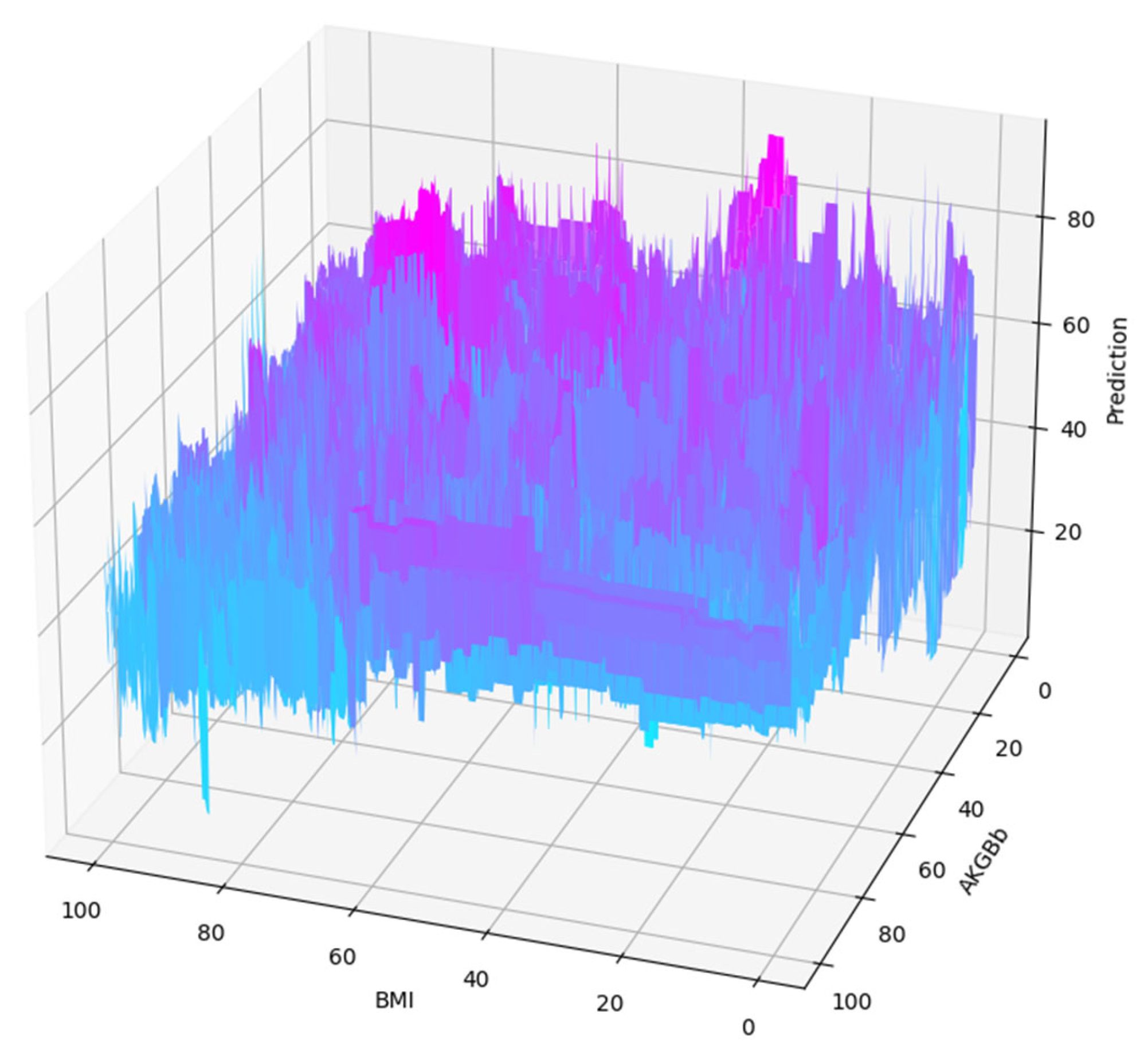
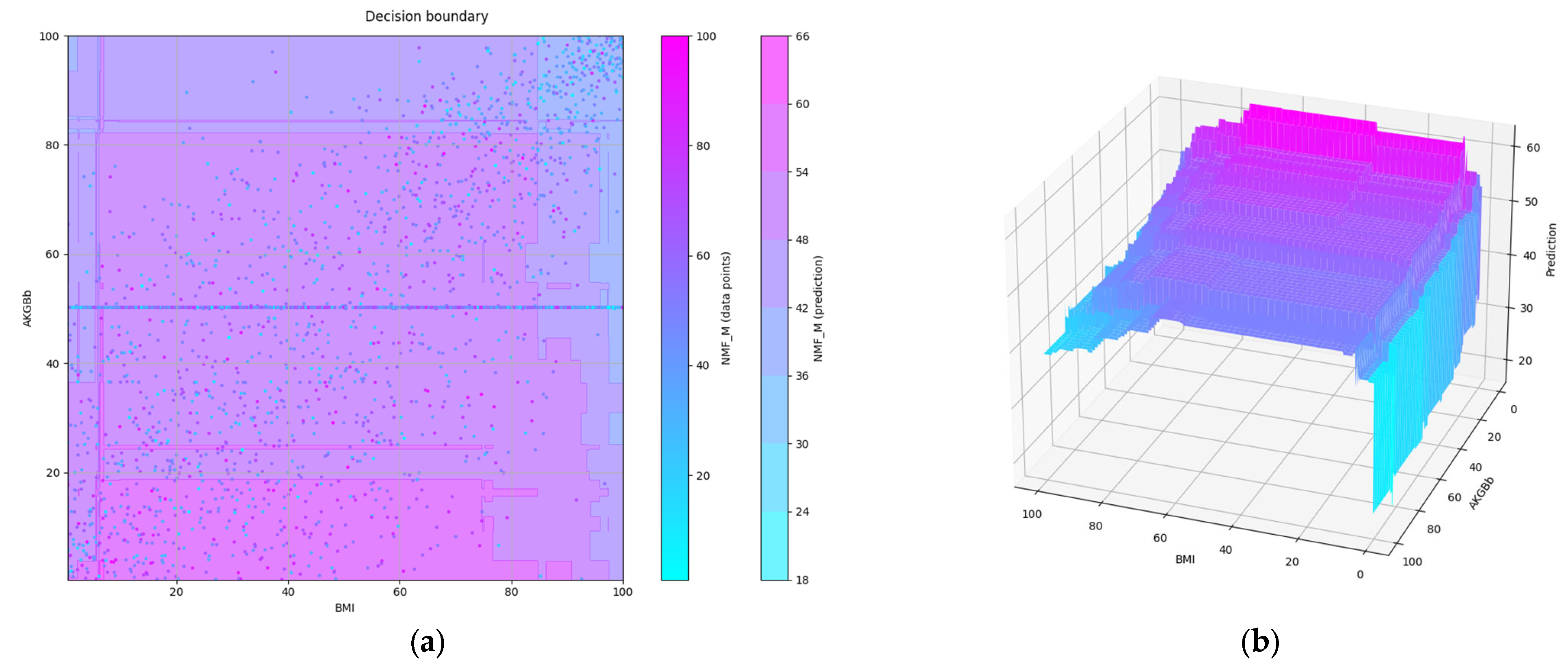
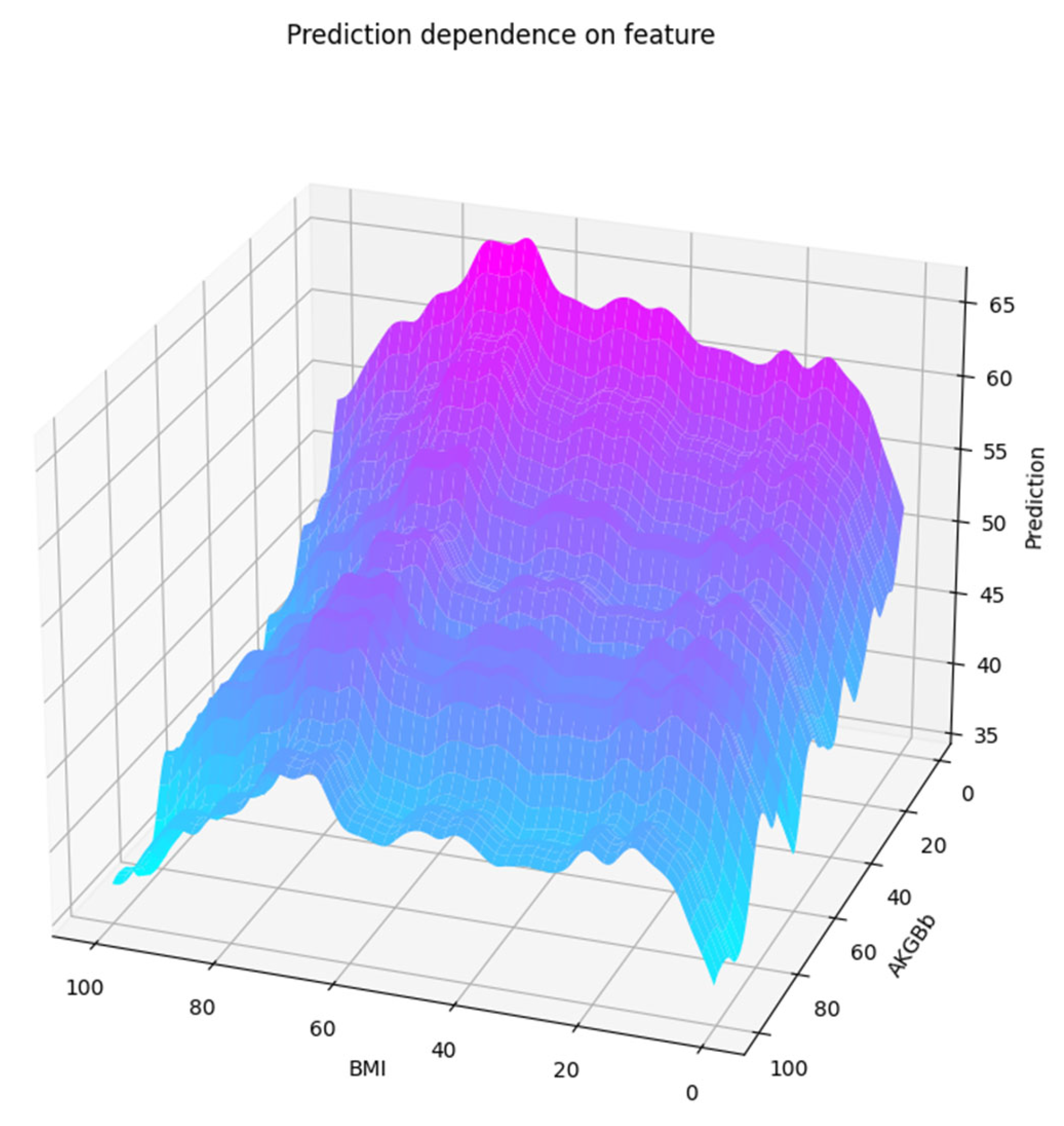
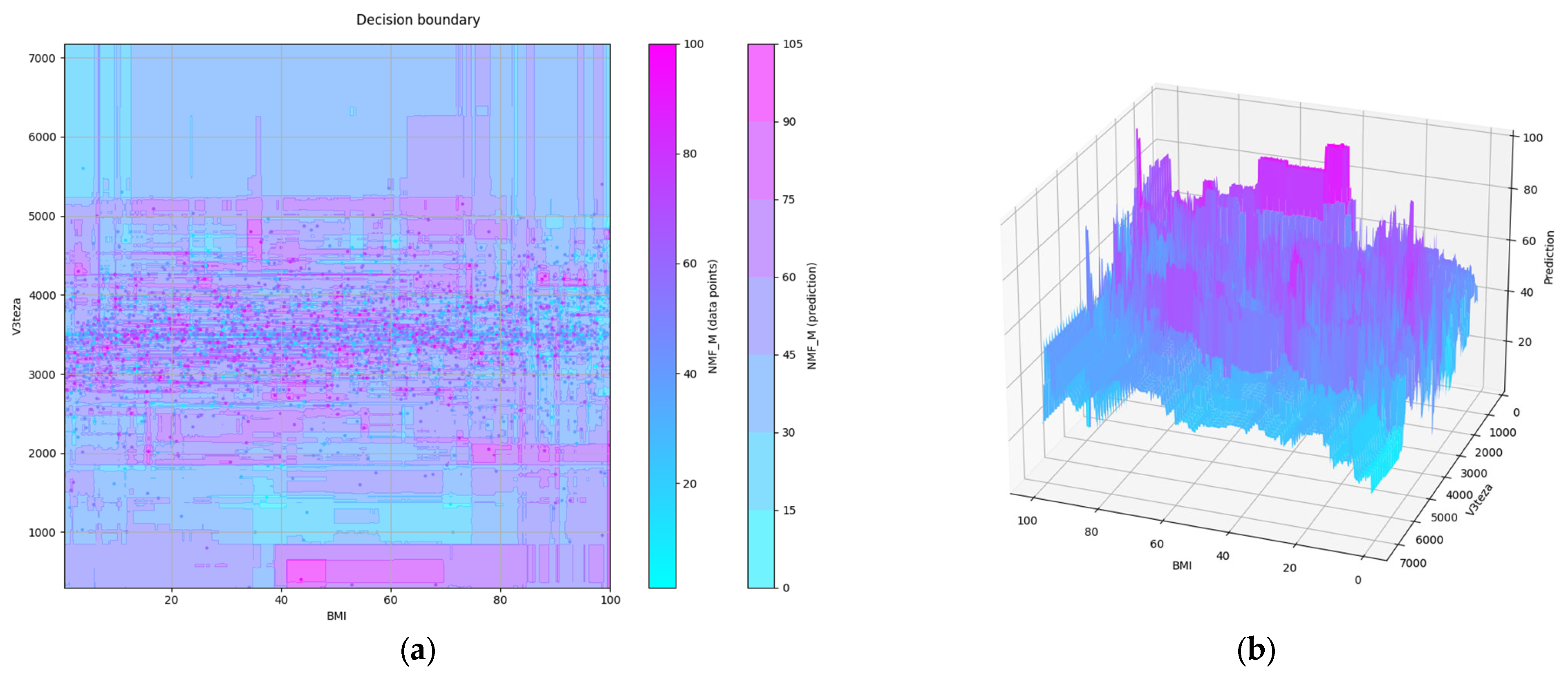
3.2. Feature Selection and Evaluation of Selected Features

The feature selection process was performed using the GFS method [6]. Initially, the hyperparameter space was retained as with the basic training process.

In the following, for the presentation to remain concise, the NMF as the MEI component will be analyzed as an example.

The first selected feature was predominantly the BMI. The relation between BMI and NMF, as modeled in the first step of the feature selection process, is displayed in Figure 2. Besides the partial dependence plot in blue superimposed over the red samples, we also show the moving average of the predicted values over ±1% of the feature values range in orange. The partial dependence plot reveals extensive jumps in prediction for even a small change in the selected feature value, which motivated us to find a smoother solution.

It is known from the theoretical foundations of gradient boosting that by tuning the number of nodes in the trees used in the ensemble, it is possible to improve the prediction of the estimator given specific data [16] (see Section 10.11). Generally, the higher values of the parameter J (implemented as max_depth in the software used) improve the prediction score. However, higher values mean large trees, which cause more computation, so it should be set around 4–8 and finetuned to achieve the best predictions. We take advantage of the fact that lower values limit the interaction between features, and in the case of value J = 2, the estimator uses only one feature in each tree.

Ensemble estimators are of a black-box nature, and for them to be more understandable, one of the explainability techniques must be used. A simple technique is visual and involves plotting a partial dependence plot, which presents the predicted value in relation to the value of a certain feature. The plot can be three-dimensional (3D) and display the interaction of a pair of features so that the prediction appears in the third dimension. A partial dependence plot in 3D becomes a partial dependence surface. Such a plot can be flattened to 2 dimensions and encode the third dimension in a color scheme.

Displaying the partial dependence plots for different, especially lower, values of hyperparameters shows the change in the behavior of the estimator. By limiting the hyperparameter space to lower values of the max_depth parameter, we can observe that the partial dependence curve flattens (see Figure 3).

At the value max_depth = 2, the predictions stay close to the average line. In this case, the relation between the BMI and predicted NMF is almost constant in the prevalent part of the range, except at percentiles lower than six and higher than 74.

The partial dependence plot at lower values of the max_depth parameter is close to the median curve of the samples, as plotted using the ExpectileGAM method, shown in Figure 4. In Python, this method from the family of Generalized Additive Models (GAM) [16] is implemented in the package pygam (the version used was 0.8.0) [17].

We show the prediction score achieved on the first step of the feature selection process because the first selected feature has the biggest prediction power. In the subsequent steps of the process, the score grows further, but the increments are smaller. Higher values of the first step score also imply fewer features needed to achieve prediction comparable to the baseline estimator. Among the score functions that are commonly used, we chose the mean squared error (MSE) because it is more intuitive than others (e.g., R²). It is implemented as negated in the Scikit-learn package to comply with the principle that a higher value is better.

Note that larger values of the hyperparameters mentioned incur more computation time.

We can see on the PDP of two features selected in the first two steps (BMI, V3teza) that MEI depends on both. V3teza is weight at birth. The PDP of these two features is shown in Figure 5, both in 2D and 3D versions. We can notice roughly three areas where lower values are predicted: at highest values of both features, high V3teza and low BMI, and low values of both features.

All the figures, 3D included, are obtained using the matplotlib [18] package, version 3.6.1. 3D figures can, at runtime, be tilted and rotated utilizing mouse dragging to understand the dependence contour’s shape better. They are all shown from the same perspective for comparison (elevation = 25°, azimuth = 110°, roll = 0°).

Other selected features show less similarity between the partial dependence plot and the median curve. Their contribution to the overall prediction is complementary—they add information through feature interaction. This conclusion also stems from the fact that the prevalent part of the score gain is obtained in the first two or three steps of the GFS process. We can indeed assume that the excellent predictions of the baseline estimator, which used all the features, are due to the multiple feature interactions and, to some extent, to overfitting.

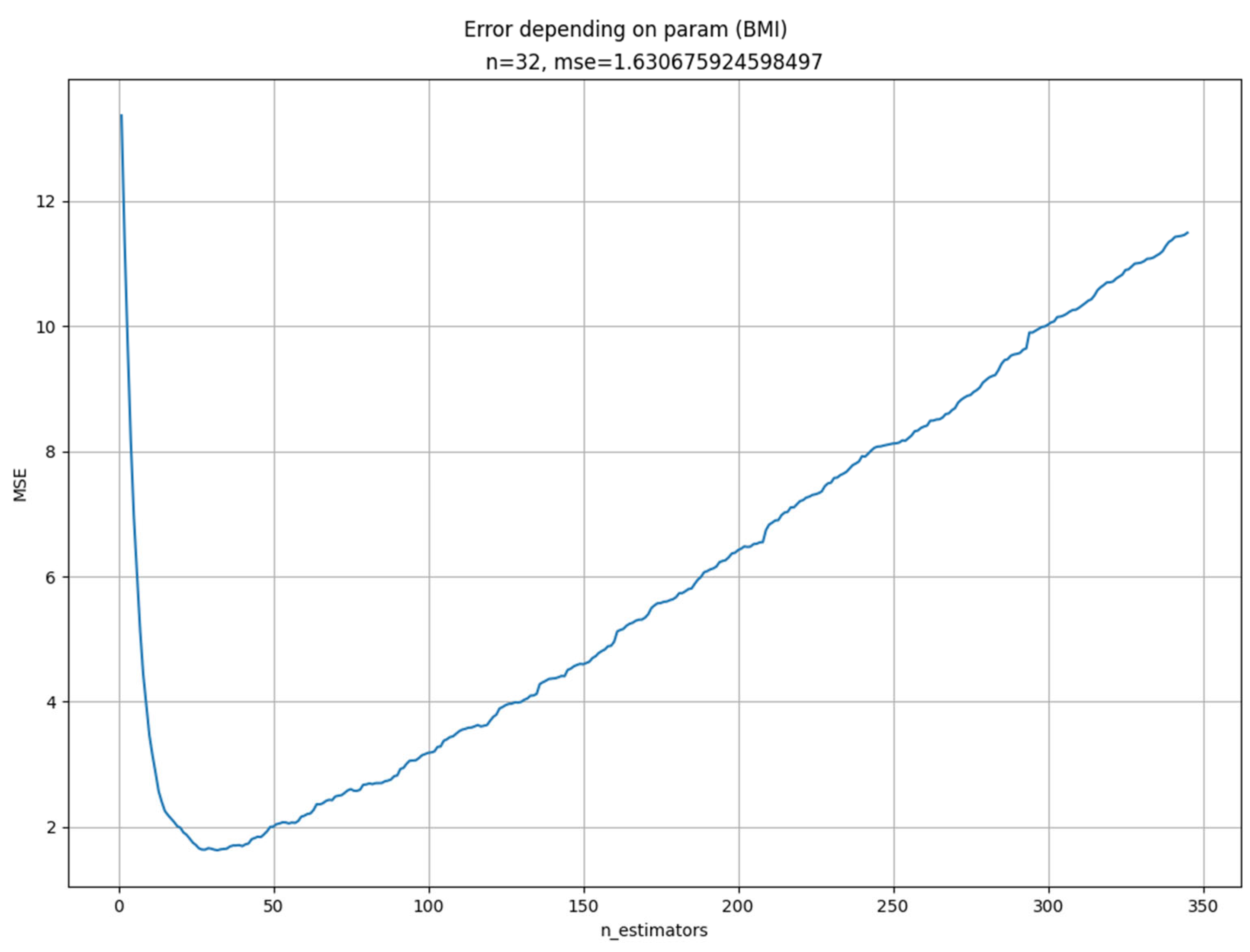
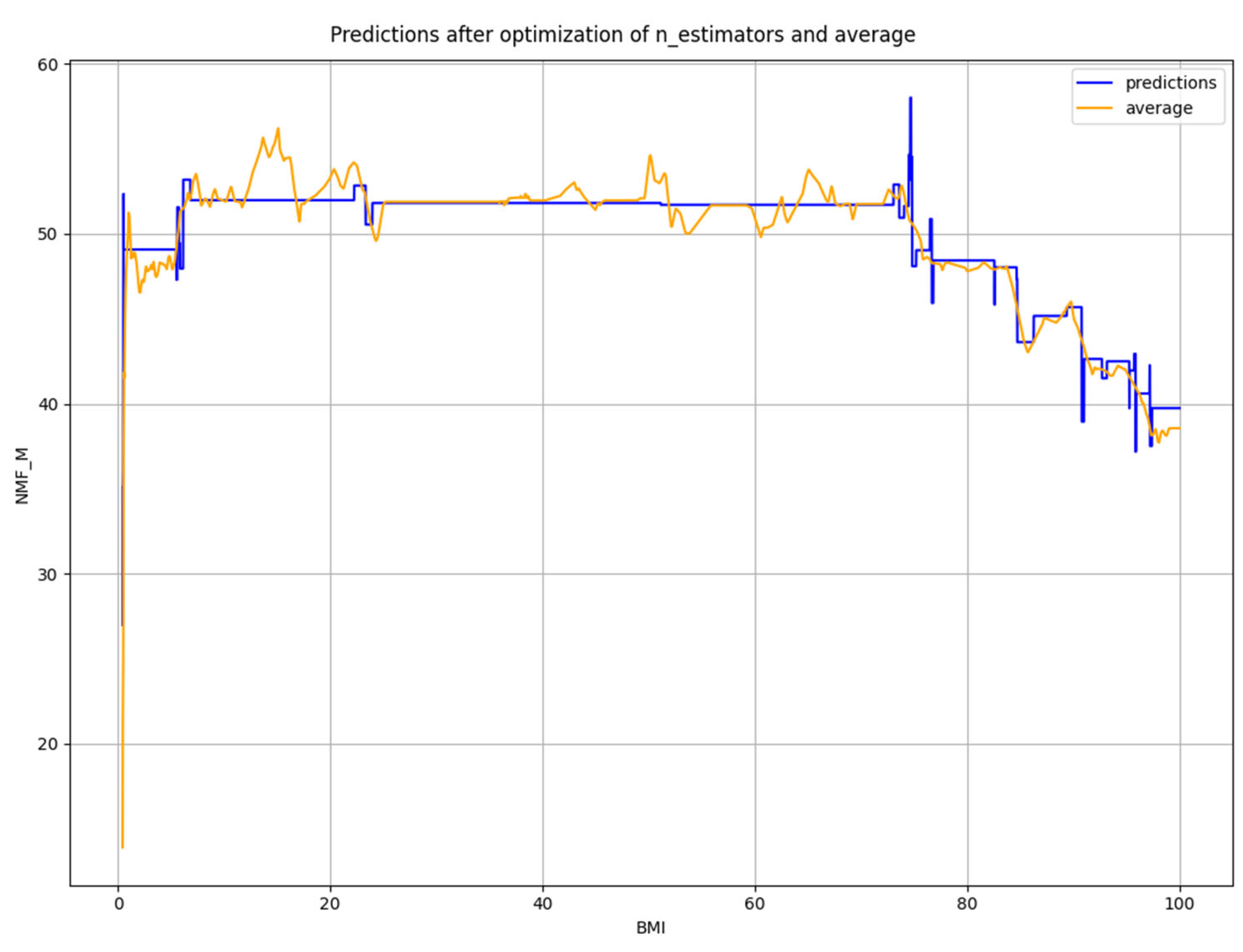
3.3. Tuning by Optimization

Increasing the n_estimators parameter to a very high level can compensate for lower prediction scores of the limited max_depth parameter, as seen in

Table 3. Prediction scores and selected features at the first step depending on hyperparameter values.

Max_depth	N_estimators	Score (MSE) at the First Step	Most Important Feature
Auto (GFS) = 16	Auto (GFS) = 128	−57.8407	BMI
9	225	−96.3913	BMI
6	225	−172.6295	BMI
5	225	−199.7296	BMI
4	225	−241.0850	BMI
3	225	−276.6921	BMI
2	10000	−51.6795	BMI
2	3200	−133.0671	BMI
2	225	−304.6900	BMI
1	10000	−311.9504	AKGNb
1	225	−329.6298	AOSG
16	100	−67.9481	BMI
16	50	−114.7980	BMI
16	25	−178.4560	ATT
16	12	−205.6439	ATT
16	6	−244.0879	ATT
16	3	−284.1534	ATT
16	2	−302.2829	ATT
16	1	−324.9178	ATT

. Decreasing this parameter helps to smooth the partial dependence plot and to get it closer to the sliding average line, but not monotonously. A minimum exists, past which the partial dependence plot departs substantially from the sliding average line. To optimize the n_estimators parameter value, we implemented a criterion function that sums the mean squared difference between the prediction for a given n_estimators parameter value and the sliding average line from GFS predictions. We performed optimization using this criterion function for all features selected in the GFS process. Because the minima for different features differ and the estimator can only take one value, we had to make a compromise, choosing the maximal one to avoid overly large errors. A typical plot of the prediction error depending on the n_estimators parameter value for the BMI is shown in Figure 6.

The smoothed prediction of NMF from BMI using the optimized n_estimators parameter value compared to the sliding average line is shown in Figure 7.

Using a limited max_depth and optimized n_estimators parameter value is also beneficial in estimating the joint influence of selected features on the predictions. In the following, we show the 3D plots of predicted values after the limiting and optimization for comparison with the one from before this process.

It is easier to discern a feature influence from a smoothed plot in Figure 8 than from the original one in Figure 5. Here, the feature interaction is more obvious and less obstructed by excessive detail.

Despite limiting the tree depth to 2, by which the individual tree depends on a single feature only, we can still observe the feature interaction because multiple trees vote for a common prediction. By optimizing the number of trees, we prevent the ensemble from adapting to detail too much.

To verify our results, we plotted the feature interaction using the ExpectileGAM method, this time in 3D. The GAM terms were set to: s(0) + s(1) + te(0, 1). This means that an additional tensor with interactions is employed in addition to linear functions of single features. We show the surface plot in Figure 9.

As observed, the gradient boosting method provides a more thorough shape of the dependence surface compared to the GAM plot. Namely, the cross-section of the GAM surface at various V3teza values has the same shape, with only minor difference in the inclination. However, its coarse shape is similar to our optimized GBR plot. This weakness is due to the fact that most GAM parameters were left at their default values; the only modification was that n_splines was increased to 200 with the s term and 30 with the te term. To improve the alignment, a deeper analysis of all the possible tuning options of the GAM models might be needed.

3.4. Spearman’s Rank Coefficient as a Source of Feature Importance Information

Calculating the Spearman’s rank coefficient between each feature and the NMF component of MEI gives us an introspection of their relatedness. The features most correlated with the output NMF are listed in

Table 4. Features with the highest absolute value of Spearman’s rank coefficient in relation to the MEI components.

NMF—M		NMF—F		MF—M		MF—F		CVF—M		CVF—F
Feature	Value	Feature	Value	Feature	Value	Feature	Value	Feature	Value	Feature	Value
AKGBb	−0.1913	AKGHb	−0.2123	AKGBb	−0.3305	AKGHb	−0.2900	BMI	−0.5327	BMI	−0.4740
AKGT1b	−0.1783	AKGGb	−0.2101	AKGNb	−0.3141	AKGBb	−0.2886	AOB	−0.5009	AKGHb	−0.4438
AKGGb	−0.1757	AKGBb	−0.1935	AKGT1b	−0.3020	AKGNb	−0.2813	AOSG	−0.4862	AOPA	−0.4269
AKGNb	−0.1736	V9M	0.1826	AKGHb	−0.3012	AKGGb	−0.2805	AOPA	−0.4771	AOSG	−0.4238
AKGHb	−0.1588	AKGNb	−0.1821	AKGGb	−0.2998	AKGT1b	−0.2396	AKGT1b	−0.4536	AOB	−0.4221
Q33	−0.1459	AKGT1b	−0.1767	AOPA	−0.2213	BMI	−0.2290	AOG	−0.4515	AKGGb	−0.4219
AOSG	−0.1457	AOPA	−0.1628	BMI	−0.2180	AOPA	−0.2208	AKGHb	−0.4501	AKGBb	−0.4218
SDQII3h	−0.1448	SDQII4d	0.1621	PSDQ3	0.2142	V5	−0.2142	AKGGb	−0.4493	AKGT1b	−0.4196
AOPA	−0.1401	BMI	−0.1588	AOSG	−0.2029	Q33	−0.2051	AKGBb	−0.4475	AKGNb	−0.4174
SDQII4d	0.1397	SDQII2l	0.1566	AOB	−0.2012	SDQII4d	0.1949	AKGNb	−0.4469	ATT	−0.4096
AOB	−0.1392	Q69	0.1565	V5	−0.2004	SDQII2l	0.1924	ATT	−0.4321	AOG	−0.3916
AOG	−0.1346	V9O	0.1546	Q33	−0.1874	V9M	0.1921	AOSS	−0.4184	AOSS	−0.3773
V5	−0.1339	V5	−0.1465	Q18	0.1814	AOSG	−0.1921	AOP	−0.4085	AOP	−0.3656
BMI	−0.1330	SDQII6g	−0.1432	Q29b	0.1787	AOB	−0.1721	V5	−0.3738	V5	−0.3468
Q29b	0.1304	SDQII1e	0.1355	ASZ	0.1765	Q69	0.1642	Q18	0.3110	ASM	−0.2889

. Interestingly, all the skin fold thickness measurements (AKG…) are near the top. They are part of the Slaughter formula [5]. Features AO… are limbs and trunk circumferences. The features whose names begin with Q…, V… and SDQ… contain results from various surveys. The position of BMI varies; in the case of NMF, it comes even at the 14th place.

Combining the BMI with all the skin fold thickness measurements manually into a smaller feature set and performing a similar analysis as above gives us the following results. The two most important features that bring in the majority of prediction score are BMI and AKGBb. Their initial 3D partial dependence plot is shown in Figure 10.

The partial dependence plot obtained after limiting the max_depth hyperparameter and optimization of the n_estimators hyperparameter is shown in Figure 11, both in 2D and 3D. Obviously, the lowest predicted values of NMF are those of samples with both high BMI and high AKGBb. According to the model, a high BMI with low values of AKGBb does not mean so much of an NMF reduction. High values of AKGBb in samples with the lowest BMI would also mean some reduction in NMF, but in practice, the number of samples with such a combination of values is low.

In fact, this feature selection is more in line with our initial goal to find features that could be a measure of the current physical status of a person and also indicate fat mass in proportion to the whole-body mass. To predict MEI, it is therefore necessary to consider both the BMI and skin fold thickness.

The GAM model of these two features is shown in Figure 12. Similarly, this plot confirms roughly the main properties of the interaction between the two features. However, it cannot capture all the interaction details as the one from the optimized gradient boosting estimator did.

4. Discussion

As only data from a single Artos measurement campaign was analyzed, the sample is rather small, which poses a problem for the machine learning algorithms. More data would mean more reliable results, as is true for the statistical methods in general. The quantity of data could be improved by combining data from several Artos measurement campaigns. Combining the data from multiple Artos campaigns would change the cross-sectional approach used in our study to a longitudinal one, requiring different methods than described here. Note that this would not constitute the typical cohort study where specific individuals are followed up. Namely, the Artos campaigns are conceived so that the nationally representative sample of school children is examined every ten years. For primary school pupils, this means that the selected individuals could not be examined twice, as the schooling period only lasts nine years (8 years before the reform in the 2000s). Special attention should also be paid to such a combined study due to its retrospective character to minimize potential confounding and bias.

As similar campaigns in other countries do not assess the same features, combining the data from different countries would mean that only a subset of features occurring in all countries could be analyzed. As shown in [3,4], some differences between populations from different parts of the world should be accounted for.

Feature interactions are of special interest in genomic studies. Here, we briefly list a few to put our work into a broader perspective.

In gene association networks, a graph is constructed by means of calculating a paCor matrix, which defines edges in the graph. If an element of the paCor matrix is nonzero, then the edge exists between respective nodes determined by matrix element indices. Study [19] develops a paCor matrix calculation method avoiding linearity and normality assumptions but still discusses a problem of feature scaling in calculations, which generally affects linear methods. The nonlinear methods like GBR which we used are not susceptible to this effect.

Study [20] describes, among others, the Multifactor-dimensionality reduction as a method of detecting gene–gene and gene–environment interactions. Its weaknesses are that it is computationally intensive, its results are difficult to interpret due to feature engineering, and the data must be balanced. Neither of these are present with the GBR method.

Another method shown to be able to uncover feature interactions is random forests. However, study [21] warns against its indiscriminate use because of the inherent problems of overlooking interactions in cases where interacting features have no marginal effect. The study lists approaches to overcome this problem known at the time of writing. We might propose the GBR as an additional candidate for this purpose.

As our method is greedy, it does not discover interactions between features that exhibit low importance in the first step of GFS. This problem was mentioned in [22]. However, in our method, interactions of these features can still influence the subsequent steps if they are related to the already selected features.

A recent review of the scientific literature in the field of gene–environment interactions shows an extensive interest in studying interactions among disparate sources of information to understand complex causal relationships better than would be possible by studying them separately [23].

5. Conclusions

In this work, we analyzed the bio-psycho-social data of children and adolescents. The data come from a long-term project, Artos, conducted in Slovenia from the decade of 1960 and still ongoing. This data have already been analyzed by the authors who conducted the project in the past. Similar campaigns are performed in other countries with similar but not identical goals and gather different sets of features.

The research question in our study was which features have the biggest influence on the MEI, by which it is possible to assess an individual’s health prospects. The most common feature used for this purpose is still BMI; however, it has been shown that BMI is not always appropriate.

To obtain a set of the most important features, we performed GFS using an ensemble estimator, in our case, the gradient boosting regressor. As this estimator’s predictions are hard to explain from the estimator parameters (black box), we used a graphical tool, partial dependence plots, to present them. These helped us to tune the estimator hyperparameters towards better generalizability. We achieve this with two measures. The first is limiting the number of nodes in the tree to two, consequently constraining the influence on predictions to a single feature. The other is by optimizing the number of trees in the ensemble on the difference between predictions and the median of feature values. Both of these can be regarded as a form of regularization. In addition to single feature importances, we show that feature interactions are a key factor in a model’s decision process. They enhance our understanding of the features and their involvement in the modeling and prediction.

Combining contributions from the most important features, we obtain a set of features that are most interesting for further study and practical work on suggestions to individuals about possible measures to improve their future well-being. Besides the body mass index, which is most frequently used currently and does not distinguish between fat and lean mass, we show that skin fold thickness measurements are the candidate features to complement it.

References

1. Wijnstok, N.J.; Hoekstra, T.; Van Mechelen, W.; Kemper, H.C.; Twisk, J.W. Cohort Profile: The Amsterdam Growth and Health Longitudinal Study. Int. J. Epidemiol. 2013, 42, 422–429. [Google Scholar] [CrossRef] [PubMed]
2. Starc, G.; Kovač, M.; Strel, J.; Pajek, M. The ACDSi 2014—A decennial study on adolescents’ somatic, motor, psycho-social development and healthy lifestyle: Study protocol. Anthropol. Noteb. 2015, 21, 107–123. [Google Scholar]
3. Cole, T.J. Establishing a standard definition for child overweight and obesity worldwide: International survey. BMJ 2000, 320, 1240. [Google Scholar] [CrossRef] [PubMed]
4. Cole, T.J.; Flegal, K.M.; Nicholls, D.; Jackson, A.A. Body mass index cut offs to define thinness in children and adolescents: International survey. BMJ 2007, 335, 194. [Google Scholar] [CrossRef] [PubMed]
5. Freedman, D.S.; Horlick, M.; Berenson, G.S. A comparison of the Slaughter skinfold-thickness equations and BMI in predicting body fatness and cardiovascular disease risk factor levels in children. Am. J. Clin. Nutr. 2013, 98, 1417–1424. [Google Scholar] [CrossRef] [PubMed]
6. Drobnič, F.; Kos, A.; Pustišek, M. On the Interpretability of Machine Learning Models and Experimental Feature Selection in Case of Multicollinear Data. Electronics 2020, 9, 761. [Google Scholar] [CrossRef]
7. Reuter, C.P.; da Silva, P.T.; Renner, J.D.P.; de Mello, E.D.; de Moura Valim, A.R.; Pasa, L.; da Silva, R.; Burgos, M.S. Dyslipidemia is Associated with Unfit and Overweight-Obese Children and Adolescents. Arq. Bras. Cardiol. 2016, 106, 188–193. [Google Scholar] [CrossRef] [PubMed]
8. Okosun, I.S.; Boltri, J.M.; Lyn, R.; Davis-Smith, M. Continuous Metabolic Syndrome Risk Score, Body Mass Index Percentile, and Leisure Time Physical Activity in American Children. J. Clin. Hypertens. 2010, 12, 636–644. [Google Scholar] [CrossRef] [PubMed]
9. DuBose, K.D.; Eisenmann, J.C.; Donnelly, J.E. Aerobic Fitness Attenuates the Metabolic Syndrome Score in Normal-Weight, at-Risk-for-Overweight, and Overweight Children. Pediatrics 2007, 120, e1262–e1268. [Google Scholar] [CrossRef] [PubMed]
10. Gutin, B. Diet vs exercise for the prevention of pediatric obesity: The role of exercise. Int. J. Obes. 2011, 35, 29–32. [Google Scholar] [CrossRef] [PubMed]
11. Adam, C.; Klissouras, V.; Ravazzolo, M.; Renson, R.; Tuxworth, W.; Kemper, H.C.; van Mechelen, W.; Hlobil, H.; Beunen, G.; Levarlet-Joye, H. EUROFIT—European Test of Physical Fitness, 2nd ed; Council of Europe, Committee for the Development of Sport: Strasbourg, France, 1993. [Google Scholar]
12. SLOfit. Available online: https://en.slofit.org/ (accessed on 26 June 2023).
13. Praprotnik, M.; Gantar, I.S.; Krivec, U.; Lucovnik, M.; Berlot, J.R.; Starc, G. Physical fitness trajectories from childhood to adolescence in extremely preterm children: A longitudinal cohort study. Pediatr. Pulmonol. 2023, 58, 1904–1911. [Google Scholar] [CrossRef] [PubMed]
14. Pedregosa, F.; Varoquaux, G.; Michel, V.; Thirion, B.; Grisel, O.; Blondel, M.; Prettenhofer, P.; Weiss, R.; Dubourg, V.; Vanderplas, J.; et al. Scikit-learn: Machine Learning in Python. J. Mach. Learn. Res. 2011, 2011, 2825–2830. [Google Scholar]
15. Scikit-Learn: Out of Bag Estimates. Available online: https://scikit-learn.org/stable/modules/grid_search.html#out-of-bag-estimates (accessed on 26 June 2023).
16. Hastie, T.; Tibshirani, R.; Friedman, J. The Elements of Statistical Learning: Data Mining, Inference, and Prediction, 2nd ed.; Springer Series in Statistics; Springer: New York, NY, USA, 2009. [Google Scholar]
17. Servén, D.C.; Brummitt, H.A. Hlink, Dswah/pyGAM: v0.8.0; Zenodo: Geneva, Switzerland, 2018. [Google Scholar] [CrossRef]
18. Hunter, J.D. Matplotlib: A 2D graphics environment. Comput. Sci. Eng. 2007, 9, 90–95. [Google Scholar] [CrossRef]
19. Andrei, A.; Kendziorski, C. An efficient method for identifying statistical interactors in gene association networks. Biostatistics 2009, 10, 706–718. [Google Scholar] [CrossRef] [PubMed]
20. Li, P.; Guo, M.; Wang, C.; Liu, X.; Zou, Q. An overview of SNP interactions in genome-wide association studies. Brief. Funct. Genom. 2015, 14, 143–155. [Google Scholar] [CrossRef] [PubMed]
21. MWright, N.; Ziegler, A.; König, I.R. Do little interactions get lost in dark random forests? BMC Bioinform. 2016, 17, 145. [Google Scholar] [CrossRef]
22. Cordell, H.J. Detecting gene–gene interactions that underlie human diseases. Nat. Rev. Genet. 2009, 10, 392–404. [Google Scholar] [CrossRef] [PubMed]
23. Virolainen, S.J.; VonHandorf, A.; Viel, K.C.M.F.; Weirauch, M.T.; Kottyan, L.C. Gene–environment interactions and their impact on human health. Genes Immun. 2022, 24, 1–11. [Google Scholar] [CrossRef] [PubMed]
Figure 1. Histogram of neuro-muscular fitness (NMF) output variable.
Electronics 12 04097 g001
Figure 2. Prediction of NMF from body mass index (BMI) at first step (red—samples, blue—prediction, orange—windowed average ± 1% of range).
Electronics 12 04097 g002
Figure 3. Prediction of NMF from BMI at first step at (a) max_depth = 6; (b) max_depth = 2 (red—samples, blue—prediction, orange—windowed average ± 1% of range).
Electronics 12 04097 g003
Figure 4. ExpectileGAM curves for NMF in relation to BMI (0.50—median).
Electronics 12 04097 g004
Figure 5. Partial dependence plot of a pair of features: (a) in 2D; (b) in 3D.
Electronics 12 04097 g005
Figure 6. Prediction error depending on the n_estimators parameter value.
Electronics 12 04097 g006
Figure 7. Smoothed prediction of NMF from BMI using the optimized value of n_estimators.
Electronics 12 04097 g007
Figure 8. Prediction related to two features after limiting and optimization.
Electronics 12 04097 g008
Figure 9. Generalized additive model (GAM) plot of predictions related to two features.
Electronics 12 04097 g009
Figure 10. Partial dependence plot of a pair of features from the smaller set in 3D.
Electronics 12 04097 g010
Figure 11. Partial dependence plot of a pair of features from the smaller set after hyperparameter limiting and optimization: (a) in 2D; (b) in 3D.
Electronics 12 04097 g011
Figure 12. GAM plot of predictions related to two features from the smaller set.
Electronics 12 04097 g012