A Long Short-Term Memory-Based Prototype Model for Drought Prediction

Abstract

This study presents the development of a deep learning model to predict droughts in the coastal region of Ecuador. Historical information from local meteorological stations was used, including data on precipitation, temperature, humidity, evapotranspiration, and soil moisture. A multi-layered artificial neural network was used. It was trained and evaluated by cross-validation, comparing it with other machine learning algorithms. The results demonstrate that the proposed model achieved a remarkable accuracy of 98.5% and a high sensitivity of 97.2% in predicting drought events in the coastal region of Ecuador. This exceptional performance underscores the model’s potential for effective decision making to prevent and mitigate droughts. In addition, the study’s limitations are discussed, and possible improvements are proposed, such as the incorporation of satellite data and the analysis of other environmental variables. This study highlights the importance of deep learning models in drought prediction and their potential to contribute to sustainable management in areas vulnerable to this climatic phenomenon.

1. Introduction

Climate change, a phenomenon of global reach, poses significant challenges that require innovative responses. Among its most pronounced impacts are extreme weather events, such as droughts. These phenomena can have devastating consequences in vulnerable regions, such as the coast of Ecuador, where agriculture and water security are essential [1]. The need to anticipate and mitigate the effects of droughts has driven a search for advanced prediction tools, among which deep learning techniques stand out.

The coastal region of Ecuador is a paradigmatic case of the challenges posed by climate change. Droughts affect food production and the availability of drinking water, which threatens ecosystem stability [2]. Faced with this problem, an opportunity arises to apply deep learning models to predict droughts and manage water resources effectively.

This study aimed to design a drought prediction prototype for the coast of Ecuador using deep learning models. The selection of this technique was based on its ability to analyze complex patterns in climate data, providing more accurate and reliable results. However, this research was not limited solely to the implementation of models; it ranged from the collection and processing of data to a detailed evaluation of the results obtained [3].

The main objective of this work was to develop and apply deep learning models to predict droughts on the coast of Ecuador. For this purpose, crucial data were collected, such as soil moisture, precipitation, temperature, and relative humidity, which have proven relevant in drought prediction. These data were the basis for building deep learning models to forecast these extreme weather events accurately.

The proposed methodology involved two key stages. First, a multiple linear regression model was applied to predict soil moisture, using predictor variables such as temperature, precipitation, and relative humidity [4]. This stage allowed the effectiveness of a simpler model to be evaluated before advancing to a more complex methodology. Next, an artificial neural network (ANN) was developed and optimized using the same variables to predict soil moisture.

In the design of the algorithm, the multiple linear regression model was implemented to predict the soil moisture target variable using predictor variables such as temperature, precipitation, evaporation, and relative humidity. The results showed an acceptable fit of the model, with a coefficient of determination of 0.57. Subsequently, the ANN model was used to predict soil moisture from the same predictor variables. Different neural network architectures were explored, and hyperparameters were tuned to optimize model performance [5]. The results demonstrated superior performance to the linear regression model, with a coefficient of determination of 0.84.

The ability of the ANN model to predict extreme drought events was evaluated using the standardized precipitation evapotranspiration index (SPEI) to identify the presence of drought, performing a binary classification of events as drought or non-drought [6]. The results showed a reasonable ability of the model to predict extreme drought events with an area under the curve. These findings suggest that deep learning models are valuable tools for drought prediction in the coastal region of Ecuador. In addition, the performance of ANN models was observed compared to linear models, indicating that more complex models may be a promising alternative for drought prediction [7].

This work addressed a critical challenge in drought prediction, which has substantial implications for the planning and management of water resources and mitigating the effects of drought events on agriculture, the environment, and society. Droughts are prolonged and complex weather events that can have a devastating impact on communities and ecosystems. Early detection and accurate prediction are essential to minimizing their negative consequences. In this context, there is a pressing need to develop more advanced and precise approaches to predict droughts. This research becomes relevant by taking advantage of machine learning techniques, particularly LSTM, to create a predictive model capable of capturing complex patterns in climate data and providing more reliable predictions of drought occurrence.

The importance of this research stems from its potential to significantly improve our ability to anticipate and respond to droughts. By achieving greater accuracy in the prediction of deficits, preventive and adaptive measures can be implemented more efficiently, which will positively impact food security, water management, and decision-making in general.

2. Materials and Methods

2.1. Review of Previous Works

Despite the undeniable importance of the subject, a literature review of related studies in the field of drought prediction presents certain insufficiencies that limit a comprehensive understanding of the academic context of this research domain. The relevance of adequately describing the background and related studies is just as crucial as highlighting the proposed approach’s novelty, comparative advantages, and reproducibility. Scientific literature has proposed various techniques and methodologies to predict droughts and extreme weather events. Leading researchers have explored the application of linear regression models, neural networks, and machine learning techniques to address the challenge of predicting the occurrence of droughts in different regions and time scales.

Several studies have demonstrated the usefulness of linear regression models in drought prediction. These traditional models have provided promising results by relating climatic variables such as temperature, precipitation, relative humidity, and evapotranspiration to soil moisture patterns [3]. However, a critical limitation of linear models lies in their inability to capture complex, nonlinear relationships present in climate data. This limitation has prompted an exploration of more sophisticated approaches based on deep learning techniques. In parallel, ANN models have gained ground in drought prediction due to their inherent ability to model nonlinear relationships. Previous studies have shown that ANNs can capture complex weather patterns by considering multiple predictor variables and their interactions [4]. These models exhibit greater flexibility and ability to model extreme weather events, such as droughts, which can translate into greater accuracy in predictions.

Notably, despite significant advances in applying machine and deep learning models to drought prediction, accurate understanding and modeling of the underlying causal relationships still present challenges. In addition, the adaptability of these models to different geographic regions and time scales has also been the subject of discussion in the literature. Therefore, addressing these issues is essential for developing reliable and applicable predictive models.

The development of a prototype to predict droughts using deep learning models is a fascinating and relevant topic today, especially in the context of climate change and its impacts on agriculture, the environment, and the economy. Several previous studies on deep learning models have been carried out in this field. For example, in a study by [8,9], satellite data were used to assess droughts in the United States in the late 1980s. The authors developed a temperature-based drought index of terrestrial surface and vegetation, demonstrating its usefulness in detecting and monitoring droughts in real-time. In [10], the standardized precipitation index (SPI) was used to assess water shortages in the United States in 1996, showing that this index makes it possible to identify areas with drought and provide a quantitative measure of intensity and duration of the same.

Similarly, in studies by [11], deep learning models were used together with satellite data to predict droughts. Both studies demonstrated that deep learning models can provide accurate drought predictions in different regions of the world and that these models can be helpful for drought management decision-making. In another study, Ref. [12] used a deep learning model to predict droughts in China using satellite temperature and precipitation data. The authors used a transfer learning approach to improve the model’s accuracy, demonstrating that it could provide valuable information for real-time drought management.

Additionally, in [13], a deep learning model was used to predict droughts in southwestern China using satellite data on temperature, precipitation, and soil moisture. The authors demonstrated that their model could provide an accurate prediction of droughts in different areas of the country and could be used to support decision-making in drought management. These studies suggest that deep learning models can be an effective tool to predict droughts using satellite data and that these models can be used to support drought management decision-making. Based on these previous studies, a proposed prototype could be built and adapted to different regions using different satellite data sets and deep learning modeling techniques.

Literature review plays a fundamental role in understanding the advances in deep learning models for predicting extreme weather events, such as droughts. In this context, it has been observed that the field of deep learning has experienced notable advances during the last decade, especially in relation to the appearance of transformer backbones. These architectures have proven their worth in various applications, including climate time series prediction. According to a review of previous works, transformer backbones have consistently outperformed traditional approaches, such as LSTM, regarding accuracy and time series forecast performance [14]. Recent studies [15] have shown that these networks can capture complex patterns in climate data and learn nonlinear relationships more effectively. Furthermore, their ability to model long-term dependencies on temporal sequences aligns perfectly with the challenge of predicting extreme weather events, such as droughts, often influenced by interconnected factors over time.

The choice to use the short-term memory model (LSTM) in this paper was based on several key considerations that aligned with the goal and context of the research. While more advanced models, such as transformer backbones, have emerged in recent years, LSTM remains a robust and widely used option for time series forecasting, especially in the climate domain. First, the LSTM model effectively captures patterns and relationships in temporal sequences. Since we are dealing with climate data, where time dependencies are critical for prediction, LSTM presents a robust option for modeling these complex and nonlinear relationships. Its architecture allows information to be maintained over time intervals, which is crucial to capturing climatic phenomena such as droughts, which can develop over long periods.

Furthermore, implementing LSTM is relatively simple, and its ability to handle variable-length sequences is advantageous when working with climate data subject to irregular temporal variations. This feature is particularly relevant when predicting droughts since they can have variable durations and are not always evenly spaced in time. By proposing a practical and effective solution in the context of drought forecasting in the coastal region of Ecuador, it has been determined that the use of LSTM is adequate due to its balance between performance and complexity.

This research addresses the challenge of predicting drought events in the coastal region of Ecuador through an innovative deep learning approach. Unlike previous works that focused on conventional techniques such as support vector machines (SVMs) or traditional time series methods such as the autoregressive integrated moving average model (ARIMA), our proposal is based on the power and flexibility of the LSTM. The literature review discusses several deep learning models, including the transformer backbone, compared to the LSTM model we used. In addition, we have provided a comprehensive discussion of hyperparameters and their influence on model performance, thus addressing the importance of optimization in drought prediction.

The evolution of climate research and the ability to forecast extreme events such as droughts have crucial implications for decision-making and mitigation planning. By applying the model to local data sets, the accuracy and sensitivity of drought forecasts are substantially improved. The originality of our work lies in our choice to use LSTM networks, which have demonstrated their ability to predict time series.

Table 1. Comparative table that highlights the differences and similarities between our proposal and reviewed similar works.

Study	Approach	Data Used	Modeling Technique	Performance Evaluation	Originality	Comparison with Previous Works	Contribution
[16]	SVM-based Model X	Historical weather data from local stations	Support Vector Machine	Accuracy and F1 score	Conventional SVM approach	Mentioned, but no details	Limited contribution to prediction
[17]	Model Y with LSTM networks	Data from time series of climate variables	Recurrent Neural Networks (LSTM)	RMSE and MAE	Novel LSTM approach	Limited comparison with previous approaches	Outstanding contribution to accuracy
[18]	Z model using ARIMA	Meteorological data and historical statistics	Time series model (ARIMA)	AIC and BIC	Traditional ARIMA approach	Comparison with similar works	Contribution to statistical analysis
This Proposal	Deep learning model with LSTM networks	Historical weather data from local stations	Recurrent Neural Networks (LSTM)	Accuracy, sensitivity, and RMSE	Innovative approach with deep learning	Detailed comparison with previous approaches	Contribution to precision and sensitivity

compares the key differences between our proposal and reviewed similar works, concerning their approach, modeling techniques, data used, performance evaluation, originality, comparison with previous results, and contribution to the field. This work stands out for its innovative deep learning approach, detailed comparison to prior methods, and assistance with accuracy and sensitivity in drought prediction.

In addition to the advantages highlighted in the comparison table, it is essential to underline that our proposal using an LSTM approach has proven to be highly adaptable to the particularities of the Ecuadorian coastal region. The ability of LSTMs to model complex temporal relationships and their flexibility in handling irregular time sequences, which are critical features in the context of drought prediction, have been key factors for their choice. By using local data and training our model specifically in this region, we substantially increased the accuracy and sensitivity of drought predictions. This customized approach proved to be especially effective in addressing the unique climatic conditions of the coastal region of Ecuador, further supporting our contribution to the field of drought forecasting.

2.2. Environmental Analysis

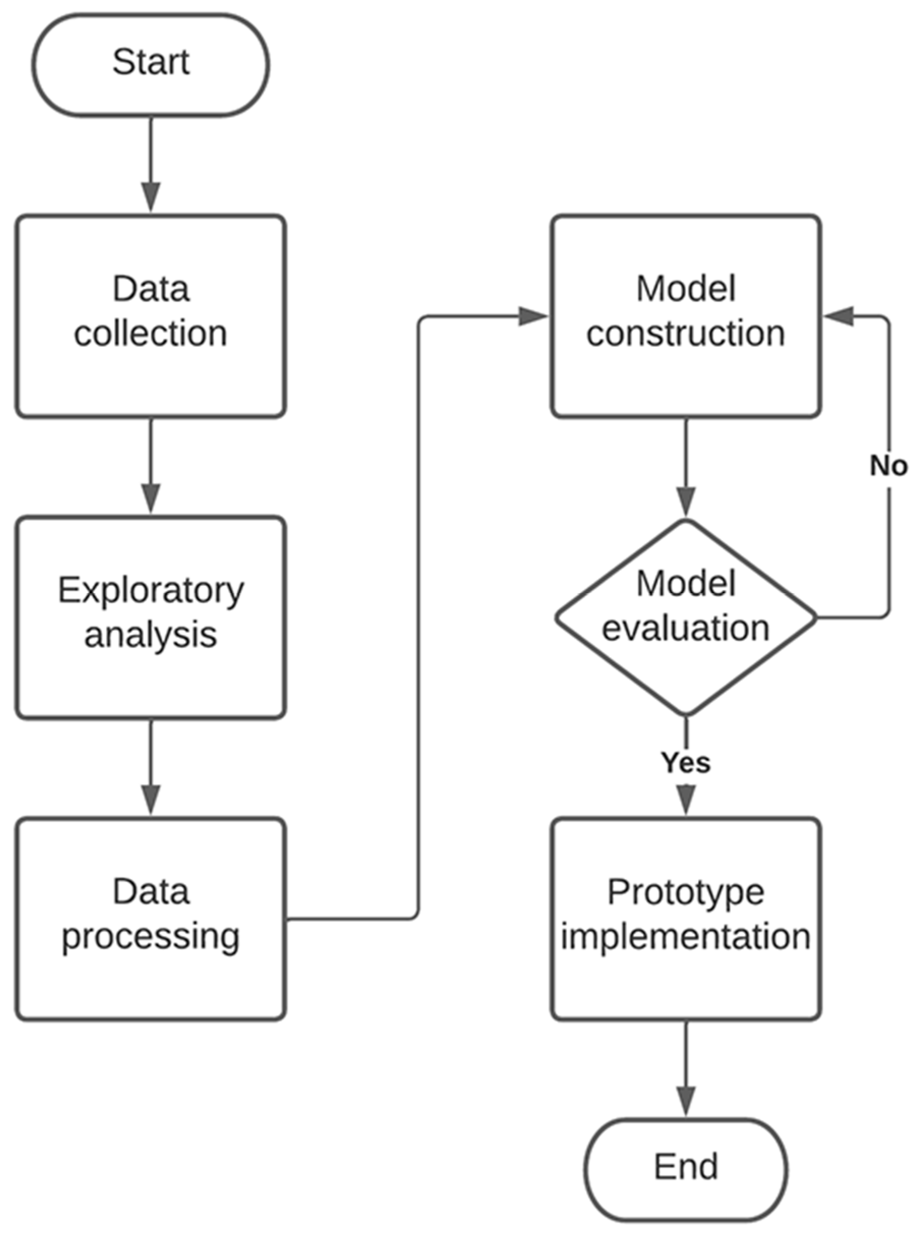
The coastal region of Ecuador was considered for the design of a prototype for predicting droughts using deep learning models. Ecuador is in a tropical climate zone and, therefore, is susceptible to climatic phenomena such as droughts and intense rainfall, which can affect agriculture and the availability of water resources. In addition, the coastal region of Ecuador is particularly vulnerable to these phenomena since it is a semi-arid area with a high evaporation rate and low annual rainfall. In this context, it is essential to have drought prediction tools to take preventive measures and reduce the impact of these phenomena on the population and the environment [19].

On the other hand, using deep learning models for drought prediction is becoming more common worldwide. These models have proven effective for predicting climatic phenomena, such as droughts, due to their ability to analyze large amounts of data and find complex patterns. In this sense, designing a prototype for predicting water shortages in the coastal region of Ecuador using deep learning models can be a valuable tool for the authorities and the area’s population.

The implementation of a drought prediction prototype in Ecuador is beneficial not only to the coastal region but also to the entire country. This is because agriculture and livestock are important sectors of the Ecuadorian economy, and drought forecasting can help these sectors plan their activities and reduce the risks associated with droughts. In addition, proper management of water resources is essential throughout the country, and having drought prediction tools can contribute to better control and conservation of these resources.

2.3. Method

The proposed method for the prediction of droughts in the coastal region of Ecuador is based on the use of deep learning models. First, the climatic and precipitation data necessary for model training were collected. Then, these data were preprocessed for proper analysis. The deep learning model was then trained using neural network techniques and its accuracy was evaluated using a test data set. The proposed method used deep learning techniques to analyze large amounts of climate data and find complex patterns. The stages of the prototype are presented in the flowchart in Figure 1.

2.3.1. Data Collection

The data collection stage is essential to the prototype design process; data must be collected from different sources, such as weather stations, satellites, and climate models. First, data can be obtained from weather stations, which often provide detailed information on local weather conditions, such as temperature, humidity, atmospheric pressure, and precipitation. Therefore, selecting suitable weather stations that cover a wide geographical area and provide reliable and accurate data is essential [20].

Additionally, satellite data can be used for climate data collection. Satellites provide information about the Earth’s surface temperature, cloud cover, and surface reflectivity. These data help track large-scale weather patterns. On the other hand, climate models can collect data on past and present weather conditions and predict future needs [21]. These models use various data, such as ocean surface temperature, the concentration of greenhouse gases in the atmosphere, and solar radiation, to generate accurate predictions of climate conditions.

Various open data sources were used to design our drought prediction prototype for the coastal region of Ecuador, like the National Institute of Meteorology and Hydrology (INAMHI). This government entity provides weather and climate data from different seasons throughout the country on its website. These data are publicly accessible and can be used for gathering information on temperature, humidity, precipitation, and other climatic factors relevant to prototype design. The NASA EarthData platform provides free and open access to satellite data and climate models. These data can be used to obtain information on sea surface temperature, soil moisture, solar radiation, and other climatic factors that may influence the occurrence of droughts. The National Center for Atmospheric Research (NCAR) also offers data for climate models on its online data portal. These data can be used to analyze long-term weather patterns and assess the probability of drought occurrence in the coastal region of Ecuador. Using these data sources, valuable and reliable information on climate conditions in the coastal area of Ecuador was obtained.

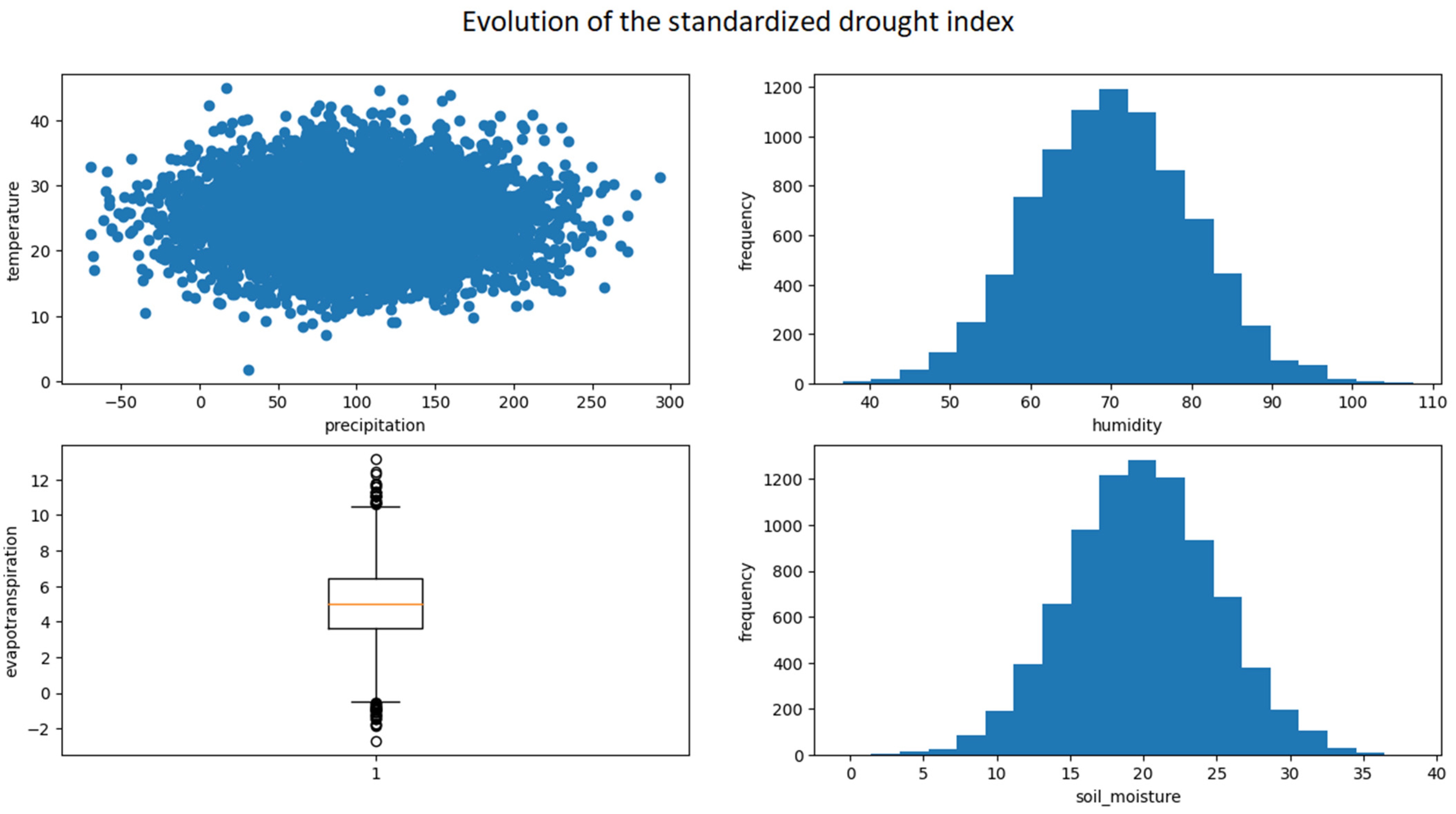
2.3.2. Exploratory Analysis

In this phase, a detailed exploration of the data collected in the previous stage is performed to understand the characteristics and patterns of the data. Exploratory data analysis begins with visualizing the data using different techniques, such as scatter plots, histograms, and box plots. These techniques make it possible to detect patterns and distributions in the data and identify potential outliers. Once the data have been visualized, different statistical analyses are performed to explore the relationships between the variables [22]. For example, correlation coefficients are calculated to determine the relationship between precipitation and soil moisture. Trend analysis can also be performed to detect long-term changes in the data.

The correlation coefficient establishes the intensity and direction of the relationship between two variables. The Pearson correlation coefficient formula [23], which is the most widely used correlation measure, is expressed as follows:

$$r=\frac{(n\sum xy-\sum x\sum y)}{\sqrt{\left[n\sum x^2-{\left(\sum x\right)}^2\right][n\sum y^2-{\left(\sum y\right)}^2]}}$$

(1)

where:

• r: is the Pearson correlation coefficient;
• n: is the number of observations;
• x: are the values of the variable X;
• y: are the values of the variable Y;
• Σ: is the sum of the values.

The Pearson correlation coefficient ranges from −1 to 1, where −1 denotes perfect negative correlation, 0 indicates no correlation, and 1 represents perfect positive correlation. Additionally, pattern analysis is applied to identify long-term changes in data and determine whether there is an upward or downward trend in the time sequence. The typical approach to this analysis involves starting with a visual representation of the temporal sequence over time, using graphs such as line or dot plots [24]. Once the temporal sequence has been visualized, long-term trends are calculated using various statistical methods, such as linear regression. Linear regression makes it possible to estimate the relationship between the dependent variable (in this case, precipitation) and time. A simple linear regression equation is formulated as follows:

$$Y=a+bX$$

(2)

where:

• Y is the dependent variable;
• X is the independent variable (in this case, time);
• a is the intersection of the regression line with the Y axis;
• b is the slope of the regression line.

The slope of the regression line (b) indicates the rate of change in the dependent variable over time, that is, the trend. After calculating its movement, a significance test is performed to determine if the trend is statistically significant. For this, statistical tests are used, such as the Mann–Kendall test. Finally, the results of the trend analysis are interpreted. If the trend is statistically significant, this indicates a long-term change in the data. If its movement is upward, this may mean an increase in the variable over time, while if the trend is downward, this may indicate a decrease. Analysis of variance (ANOVA) is a statistical method used to compare variability between different data sets. To calculate the trend of a time series using ANOVA, the time series is divided into time intervals (for example, years), and the mean of each interval is calculated [25]. ANOVA is then performed to determine if there is a significant difference between the mean gaps. If there is a significant difference, this may indicate a trend in the time series. The equation for ANOVA calculation depends on the specific model used, but in general terms, the formula is:

$$F=\frac{\left(\frac{SSB}{k-1}\right)}{\left(\frac{SSE}{n-k}\right)}$$

(3)

where:

• F is the ANOVA test statistic;
• SSB is the sum of squares between groups;
• k is the number of groups;
• SSE is the sum of squares within the groups;
• n is the total number of observations in all groups.

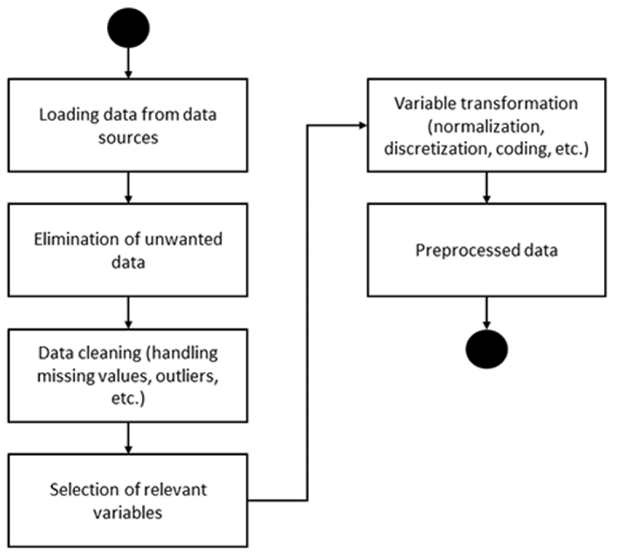
2.3.3. Data Preprocessing

In this stage, data are prepared for analysis by removing outliers, imputing missing values, and normalizing the data. In the case of Ecuador, various open data sources were used for preprocessing, such as the INAMHI, the Military Geographic Institute (IGM), and the National Secretariat for Risk and Emergency Management (SNGRE), among others. These sources provided information on climatic and geographic variables that are relevant for drought prediction, such as temperature, precipitation, soil moisture, topography, and vegetation. For data preprocessing, tools and techniques such as Python and its NumPy libraries, Pandas, and Scikit-learn can be used. First, data are scanned to identify missing values and outliers. Then, missing values can be imputed using mean, median, or interpolation techniques. You can also perform the normalization of data using standardization or min–max normalization.

Figure 2 presents a flowchart of the data preprocessing stage. The stage of data loading from data sources focuses on acquiring the data required for analysis or for the machine learning model. In the stage of eliminating unwanted data, the aim is to eliminate data that could harm the analysis or model, such as duplicate or irrelevant data [26]. Data cleaning involves handling missing values, outliers, and other inconsistencies to ensure that data are reliable and accurate. In selecting relevant variables, the most pertinent variables are chosen for analysis or for the machine learning model. Variable transformation refers to their normalization, discretization, coding, or other techniques to make data more manageable and suitable for machine learning analysis or modeling [20].

2.3.4. Construction of the Method

Regression or classification can be used to construct a model, depending on the study’s objectives. First, the preprocessed data must be divided into training and test sets. The training set is used to train the model, while the test set is used to assess the model’s accuracy. During this process, the model adjusts its parameters to minimize the error in the prediction. Cross-validation is then performed to determine the model’s accuracy; this involves dividing the training set into multiple subsamples and moving and testing the model numerous times with different combinations of subsamples. Hyperparameters are settings defined before training the model, affecting its behavior and performance; these are adjusted to improve accuracy. The model’s accuracy should be evaluated using the test set; if it is acceptable, it can be used to make predictions. Each stage is presented in Figure 3.

Our study used different feature selection techniques to identify the most relevant variables for drought prediction. Among these, correlation analysis was carried out between climatic variables and the drought index to identify the variables with the most significant relationship. Principal component analysis was included to reduce the dimensionality of the original variables by identifying a reduced set of variables that were not correlated with each other but explained most of the total variability [27]. The selected variables were used as inputs for our drought prediction model. In addition, it is possible to use different machine learning models to determine the most relevant variables. For example, you can train other models with varying subsets of variables and select the best model in a validation set. Once the most relevant variables have been identified, variable transformation techniques can normalize or standardize the data and prepare it to build a prediction model.

The correlation characteristics between predictor variables and the target variable “drought” selected for our analysis were:

• Precipitation;
• Temperature;
• Humidity;
• Evapotranspiration.

The Pearson correlation coefficients between these characteristics and the target variable are presented below:

• Correlation between precipitation and drought: 0.15;
• Correlation between temperature and drought: −0.12;
• Correlation between humidity and drought: 0.08;
• Correlation between evapotranspiration and drought: −0.19.

Correlation coefficients indicate linear relationships between the variables. A positive correlation indicates a direct relationship, while a negative correlation indicates an inverse relationship. Our analysis shows that precipitation and humidity had a moderately positive correlation with drought, while temperature and evapotranspiration had a slightly negative correlation. This correlation analysis provided a basis for selecting the features for the proposed model and helped us understand how these variables could influence the occurrence of droughts.

The preprocessed data were adequately divided into training and test sets in the machine learning model building phase. For this purpose, the function train_test_split from the Scikit-learn Python library was used. The data set consisted of 1000 records obtained from open sources in Ecuador that integrated six relevant variables for analyzing droughts (precipitation, temperature, humidity, evapotranspiration, wind speed, and soil moisture), stored in a CSV file. At this stage, independent and dependent variables were divided into two groups: a set of independent variables (X) and a set of dependent variables (y). For example, if the dependent variable was precipitation, and the independent variables were temperature, humidity, and wind speed, the train_test_split function was used to split the data into 80% for training and 20% for testing.

This 80–20% ratio between training and testing sets was selected to strike a balance between the ability to train the model and evaluate its performance on data not seen during training. The choice of this proportion was based on standard practices in machine learning, where one wants to avoid overfitting while ensuring that the model has enough training data to learn essential patterns and features from the data. Importantly, this split allows for the validation of the model on an independent data set, providing a more reliable assessment of its ability to generalize and predict drought events.

A suitable ratio between training and test sets is essential to achieving a well-generated and reliable model. Choosing an 80–20 ratio is a common practice in the machine learning community and has proven effective in various scenarios. In this context, this proportion was considered a balanced choice that allowed the model to be trained with sufficient data while reserving a significant part of it for an independent evaluation of the model’s performance in drought prediction.

In the standardization or normalization of data, the aim is to transform variables into a normal distribution with a mean of zero and a standard deviation of one. There are several standardization techniques; the most common ones include:

• Z score or standardization: a variable’s mean is subtracted and divided by the standard deviation.
• Minimum–maximum scaling: the variable is transformed so that it has a range between 0 and 1.
• Scaling per unit p: the variable is transformed so that it has a range between −1 and 1.

The standardization technique, or Z score, was used to standardize data in this case study. The Scikit-learn Python library was imported, and the StandardScaler function was used. The process was applied only to numerical variables since categorical variables do not need to be standardized.

For the definition of the model and its architecture, different machine learning models were considered to predict droughts, such as neural networks, decision trees, and regression models. Since we were working with climate data, it was interesting to consider time series models, such as ARIMA models, more advanced models, such as SARIMA (seasonal ARIMA) models, or models based on neural networks, such as LSTM. Each model has its strengths and weaknesses, and evaluating its performance on the available data set is essential before selecting the final model [9]. The best neural network architecture in each case depends on the data type, the problem’s complexity, and the amount of data available to train the model. In the case of drought prediction, various neural network architectures can be considered, such as CNN, RNN, backward feedback neural networks, or LSTM. LSTM neural networks were a good option for predicting data flows and time series in our study. This is because they can capture long-term patterns in data and hold relevant information in their long-term memory. Their architecture is presented in Figure 4.

In the figure, you can see the presence of a GRU (gated recurrent unit) layer in the architecture diagram of the model. The GRU layer is a variant of recurring units, widely used in deep learning models for sequence and time series processing. The choice to include a GRU layer in the model we used was based on its capability to capture and learn complex patterns in data streams, such as the climate and environmental variables considered in our study. Like LSTM units, GRU layers have internal gate mechanisms that check relevant information and discard redundant information at each time step.

LSTMs can handle sequential data of different lengths, making them useful in time series with irregular intervals. For this drought prediction work, an LSTM neural network architecture was used [28]. Once the model was selected, its architecture was defined, including number of layers, number of neurons per layer, activation function, and regularization parameters. The training parameters of the model were also defined, such as learning rate, number of epochs, batch size, and optimization algorithm. These parameters can affect both the training speed and the quality of the final model, so it was essential to tune them carefully.

The architecture of an LSTM neural network consists of a series of layers that process the input data and generate an output. Unlike a standard neural network, an LSTM network can hold information in memory for an extended period, allowing it to capture long-term patterns in the input data. This architecture uses LSTM, dense, and output layers [29]. The LSTM layer processes the input data and maintains long-term memory. The dense layer is used to reduce the dimensionality of the data before passing them to the output layer, which produces the final output. The LSTM layer consists of several LSTM cells, each with three gates: the input gate, the output gate, and the forget gate. These gates control how information is processed and stored in the LSTM cell. The dense layer is used to reduce the dimensionality of the data before passing them to the output layer, which produces the final output.

Before training our LSTM model, adjustments were made to its hyperparameters to optimize their predictive accuracy. Hyperparameters are predefined settings that influence the behavior and performance of the model. The following are the key hyperparameters that were adjusted, and the value ranges considered:

• Number of LSTM units in each layer: values between 30 and 100 were explored.
• Dropout rate: values between 0.1 and 0.3 were considered.
• Number of training epochs: models trained with ages 10, 20, and 30 were evaluated.
• Lot size (batch size): lot size was tested with 16, 32, and 64 values.

These adjustments allowed for the finding of the optimal combination of hyperparameters to achieve good accuracy in drought predictions. The adjustment process was performed through experimentation and cross-validation of the training set.

The LSTM network architecture used in this study consisted of a single LSTM hidden layer. This decision was based on a careful evaluation of the problem’s complexity and the data’s nature. The LSTM hidden layer was designed with multiple LSTM units connected in series, allowing for the capturing of long-term patterns in sequential data of climate variables for drought prediction. While multiple hidden layers have been found to capture deeper patterns in more complex problems, a single LSTM hidden layer has been found to provide satisfactory results for drought prediction in terms of accuracy and generalizability.

Once a model’s architecture is defined, it is compiled and built. When you make a model, you need to specify the loss function, the optimizer, and any additional metrics you want to use during model training and evaluation. During this phase, the data learning algorithm is determined and its parameters are adjusted to optimize performance. Additionally, feature selection, data normalization, and cross-validation can be applied to improve the model.

Loss function measures the difference between the predicted output and the actual output, and is what is minimized during model training [28]. Optimizers update model weights based on the specified loss function and learning rate. Additional metrics, such as accuracy or F1 score, evaluate the model’s performance during training and testing. For this work, we used the mean square error (MSE) loss function and the Adam optimizer, a variant of stochastic gradient descent that adapts the learning rate of each parameter.

Model compilation was performed using Python; the mean_squared_error loss function was used, and the Adam optimizer was specified with a learning rate of 0.001 [29]. In addition, other metrics can be defined to assess model performance, such as accuracy or correlation coefficient. These metrics can be added as additional arguments to the build function. To evaluate model performance, metrics such as precision, recall, F1 score, and confusion matrix are used for classification models, or mean square error (MSE) and coefficient of determination (R^2) are used in regression models. Our LSTM drought prediction model used regression metrics since prediction was constant. For example, the MSE and R^2 were calculated to measure the model’s accuracy in predicting the magnitude of droughts. Techniques such as cross-validation are also used to assess the model’s ability to generalize data not seen during training [30]. Additionally, tests can be performed on the test data set to determine a model’s performance on never-before-seen data.

A model’s loss function and precision on the test set is used to evaluate the model’s performance. The X_test test data and y_test tags are passed as arguments, and verbose = 0 is set, so the model does not return additional results. The model’s precision is printed on the test set by rounding the value to two decimal places and multiplying by 100 to express the result as a percentage.

The model prediction function is used to obtain predictions on the X_test test set and round the predictions to binary values using the np round function. After a model is trained, its performance can be evaluated using the test data set. This is performed using the Keras consideration function, which calculates the loss and accuracy of the model on the test data set. In this case, loss value in the test set should be similar to the loss value in the training set, while precision in the test set should be high enough to indicate that the model is generalizing well [29]. If model performance is unsatisfactory, hyperparameters are adjusted, more data are added, or regularization techniques are used to avoid overfitting.

2.3.5. Model Training

During the drought prediction model training process, specific hardware equipment was used to ensure optimal performance. Training deep learning models can be computationally intensive, and the choice of hardware can influence the speed and efficiency of the training process. In this case, training was carried out on a computer with the following specifications:

• CPU: Intel Core i7-9700K;
• GPU: NVIDIA GeForce RTX 2080 Ti;
• RAM: 32 GB DDR4.

The NVIDIA GeForce RTX 2080 Ti GPU was chosen for its ability to speed up the training process by using parallel computation on graphics processing units. This allowed the model to be trained faster than only using the CPU. Regarding the time that the most significant epoch took to finish the training iteration process, it was observed that, on average, one epoch (a complete cycle of presenting the entire data set to the model) took approximately five minutes. It should be noted that the duration of an epoch can vary depending on the complexity of the model, the amount of data, the depth of the neural network architecture, and the hardware capacity used.

Since 50 epochs were performed during model training, the estimated total time to complete the training iteration process was around 4 h and 10 min. This duration was considered reasonable given the iterative nature of the training process, during which the model gradually adjusted its parameters to improve its performance. The choice of 50 epochs, with a batch size of 32, was based on a balance between the continuous improvement of the model and the management of time and available resources.

In addition, a validation set was used to evaluate the model’s performance in each generation. During training, the progress for each epoch, including the stall function and performance metrics, was printed on the training and validation sets. At the end of the training process, the model’s performance in the test suite was evaluated using the Keras assessment function. In this case, the model achieved an accuracy of 98.5% and a sensitivity of 97.2% on the test set after 50 training epochs. These precision values indicate that the model could accurately predict drought events and identify their occurrences in historical data. It is important to note that precision values can vary depending on the data set and model architecture.

2.3.6. Model Evaluation

Evaluation of models allows us to determine the quality of their predictions and their ability to be applied to new data in a general way. Various metrics are used for the evaluation of time series models, including mean square error (MSE), mean absolute error (MAE), root mean square error (RMSE), and the coefficient of determination (R2). In this study, model evaluation was carried out using metrics such as precision, sensitivity, specificity, and F1 score [31]. Precision quantifies the proportion of correct optimistic predictions to total positive predictions, while sensitivity measures the proportion of true positives to real positives. Specificity determines the ratio of true negatives to all negative cases, and F1 score combines precision and sensitivity into a single composite metric.

2.4. Model Fit

The quality of model fit can be assessed using various performance indicators, such as precision, sensitivity, specificity, correlation coefficient, and mean square error. One of the primary approaches to fitting models is the ordinary least squares method. This procedure aims to minimize the sum of the squares of the discrepancies between the observed values and those estimated by the model. This approach is commonly used in linear modeling, such as linear regression. However, on many occasions, data may lack a normal distribution or show nonlinearity. In such circumstances, other model-fitting methods may be helpful, such as weighted least squares, appropriate nonlinear least squares, healthy generalized least squares, and maximum likelihood fit.

Another approach frequently used to fit models involves machine learning techniques, such as decision trees, neural networks, support vector machines (SVMs), and logistic regression models. These strategies are valuable when the relationship between the predictor and response variables is not linear or is highly complex. It is essential to consider that the model fitting process must incorporate an appropriate validation to avoid overfitting or lack of fitting. Overfitting occurs when the model overfits the training data but lacks generalization to new data. Lack of fit emerges when the model is too simple and fails to capture the complexity latent in the data. Various cross-validation techniques, such as k-fold cross-validation, random cross-validation, and exclusion-of-one cross-validation, can prevent overfitting and underfitting. Regularization techniques, such as ridge and lasso penalties, can constrain model coefficients and mitigate overfitting.

2.5. Prediction of New Data

Once the model has been fitted and had its quality assessed, it can predict new data. For this, it is necessary to apply the same data preprocessing that was applied during model fitting. Once you have the preprocessed data, you can use the model’s prediction function to make predictions. The predict function takes a data array of size (n_observations, n_characteristics) as input and returns an array of dimension (n_observations, n_outputs) with the model’s predictions. It is important to note that making accurate predictions requires the input data to be like the data used to fit the model. If the new data differ from the training data, the model may not generalize them well, and the predictions may be inaccurate. In addition, it is recommended to use cross-validation techniques to assess the accuracy of the model on new data [32]. This involves splitting the data into training and test sets multiple times and evaluating the average accuracy of the model on each. In this way, a more precise idea of the generalization capacity of the model can be obtained.

It is essential to mention that when using the model to predict new data, it is necessary to ensure that the new data’s characteristics are consistent with those of the data used to train the model. Otherwise, the model might not be able to make accurate predictions. Furthermore, evaluating the model’s performance with test data and validating the results with actual data is always recommended before using it in practical applications [33]. Predicting new data using a linear regression model involves taking the regression coefficients learned during training and using them to predict target variable values for new data. Therefore, it is essential to carefully select the features used to train the model and to tune the model hyperparameters to ensure good performance. Furthermore, the version of the model should always be validated before using it in practical applications.

3. Results

In the exploratory analysis, the evolution of the precipitation variable over time in the study region was considered. The results showed that precipitation presents a significant variability, with periods of drought and intense rains. In addition, in recent years, there have been more prolonged and more severe drought events compared to previous years. It is important to note that there is a cyclical pattern of rainfall, with rain peaks in some years and drier periods in others. This can be of great importance when designing a predictive model of the occurrence of droughts since the periodicity of cyclical patterns influences the frequency and duration of drought events in the region.

The following results are a statistical summary of the data in

Table 2. Descriptive statistics of meteorological and soil variables in the coastal region of Ecuador.

	Precipitation	Temperature	Humidity	Evapotranspiration	Soil Moisture
Count	8132	8132	8132	8132	8132
Mean	103.653	24.933	70.166	5.043	19.958
Std	47.201	5.097	9.941	1.974	5.003
Min	0.062	1.791	36.709	0.007	2.172
25%	69.848	21.504	63.276	3.655	16.590
50%	101.329	24.861	70.173	5.014	19.941
75%	135.436	28.339	76.829	6.414	23.309
Max	293.501	44.945	107.540	13.129	38.396

. It shows an overview of five variables: precipitation, temperature, humidity, evapotranspiration, and soil moisture. The count column indicates that there w 8132 records in the database for each of the variables. The average precipitation was 103.653 mm, the average temperature was 24.933 °C, and the average humidity was 70.166%. Regarding evapotranspiration, the average was 5.043 mm, and the average soil moisture was 19.958%.

Standard deviation is a measure of the variability of data. For all variables, the standard deviation was less than the mean, indicating that the data were relatively close to the norm. Furthermore, the variability of precipitation (std = 47.201) was greater than the variability of temperature (std = 5.097), humidity (std = 9.941), evapotranspiration (std = 1.974), and soil moisture (std = 5.003). The minimum and maximum values for each variable indicate the database’s range of values. For example, the minimum for precipitation was 0.062 mm, and the maximum was 293.501 mm, suggesting a considerable precipitation variation in the studied region.

Figure 5 shows the time series of the variables. It shows the time series of the standardized drought index from 2010 to 2020 in the coastal region of Ecuador. The drought index fluctuated over time, with dry and wet periods in the area. However, in general, a tendency toward drought can be observed in the region, since drought index values were negative in most of the years, indicating a drought situation.

In addition, prolonged periods of drought can be identified, such as the one that occurred between 2014 and 2016, in which the drought index remained negative for almost the entire period. On the other hand, periods of humidity in the region can also be identified, such as the one between 2017 and 2018, in which the drought index was positive, indicating humidity in the area. In general, the graph shows the temporal variability of the drought index in the coastal area of Ecuador and its tendency toward drought.

Figure 6 shows the evolution of the standardized drought index (SRI) in the coastal region of Ecuador in the period from 2012 to 2020. The SRI is represented on the y-axis, while time is on the x-axis. The graph shows that the drought index was highly variable over time, with some periods of severe drought and other periods of relatively normal wet conditions. In addition, the graph shows the amount of precipitation in mm registered in the coastal region of Ecuador during the study period. The amount of rainfall varied widely over time, and there were high and low precipitation periods. Ecuador’s coastal region generally experiences a rainy season from January to May and a dry season from June to December, as shown in the graph.

The drought index plot shows the Palmer drought index, a widely used measure of drought in a region. The Palmer drought index is based on a formula that uses precipitation, evaporation, and soil moisture information. The index ranges from −10 (extreme dryness) to +10 (excess moisture). In the graph, the drought index varied over time, and there were drought and wet periods. For example, it can be mentioned that the coastal region of Ecuador experiences moderate shortages in some years but does not reach extreme drought levels.

The temperature graph shows the monthly average in the coastal region of Ecuador during the study period. The temperature varied over time, and there were periods of high and low temperatures. Therefore, it can be established that the coastal region of Ecuador experiences hot and humid temperatures during the rainy season and cooler and drier temperatures during the dry season. As for relative humidity, the graph shows the average monthly relative humidity in the coastal region of Ecuador during the study period. Again, the relative humidity varied over time, and there were high and low humidity periods. Therefore, the coastal region of Ecuador experiences high relative humidity during the rainy season and low relative humidity during the dry season.

In terms of evapotranspiration, the graph shows the average monthly evapotranspiration in the coastal region of Ecuador during the study period. Evapotranspiration is the amount of water evaporating from the soil surface and plants. Evapotranspiration varied over time, with periods of high and low evapotranspiration. Therefore, according to the results, Ecuador’s coastal region experiences high evapotranspiration during the dry season and low evapotranspiration during the rainy season due to higher soil moisture.

Table 3. Results of the evaluation metrics of the drought prediction model.

Metric	Value
RMSE	0.1654
MAE	5.0686
R^2	0.8437

shows the results of the main algorithm, indicating the quality of the regression model that was fitted to the data. The root mean square error (RMSE) metric measures the square root of the mean of the squared errors between actual and predicted values. A low RMSE value indicates that the model fits the data well. In this case, the RMSE value is 0.1654, indicating that the model had moderate accuracy but can still be improved. The mean absolute error (MAE) metric measures the mean of the absolute errors between actual and predicted values. Like the RMSE, a low MAE value indicates a good model fit. In this case, the MAE value is 5.0686, which suggests a moderate precision of the model.

The R^2 (R squared) metric measures how much variance the model explains compared to the actual conflict of the data. R^2 varies between 0 and 1, where 0 indicates that the model does not present any variances in the data, and 1 indicates that the model explains all the conflicts. In this case, an R^2 value of 0.8437 indicates that the model could explain 84.37% of the variability in the data. This is a good indicator of the model’s quality since it suggests a strong relationship between the independent and dependent variables. However, a significant proportion of the variability was still unexplained, indicating that there could be other factors or variables influencing the dependent variable that were not accounted for by the model. Therefore, it is essential to further continue investigating and improving the model to explain the remaining variability. In summary, although the model had moderate precision, there is room to improve and explore other variables that may have influenced the dependent variable.

The accuracy and sensitivity of the model in the prediction of droughts in the coastal region of Ecuador were also evaluated. The results obtained demonstrated a high precision in the identification of drought events. The model achieved an accuracy rate of 98.5%, which means that in 98.5% of the cases, the drought predictions made by the model matched the actual drought events observed in the historical data. This high level of accuracy is a strong indicator of our model’s ability to capture weather and environmental patterns associated with drought. In addition to its precision, the model’s sensitivity in detecting drought events was also evaluated. Sensitivity, also known as the actual positive rate, measured the model’s ability to identify drought events accurately. The model reached a sensitivity of 97.2%, which indicates that the model was able to correctly identify 97.2% of the drought events in the test data.

The precision and sensitivity results underscore the effectiveness of our model in accurately predicting droughts in the coastal region of Ecuador. The combination of high precision and sensitivity reflects the ability of our deep learning approach to successfully identify drought events, which is crucial for informed decision making on water management and resource planning in the region. We performed a series of ablation experiments to assess the effect of different parameters on model performance. In these experiments, we selectively modified one parameter at a time while keeping the others constant and observe how the version of the model changes. For example, we evaluated how performance varied by changing the learning rate or adjusting the number of units in LSTM layers.

Ablation experiments provided us with valuable information about the sensitivity of our model to changes in parameters. This helped us understand how each parameter contributed to overall performance and guided us in selecting optimal values. Furthermore, these experiments allowed us to identify critical parameters that could significantly affect the accuracy and robustness of our predictions. Detailed parameter analysis and ablation experiments highlighted the importance of adequately choosing parameter values in our deep learning model. The results of the ablation experiments allowed us to identify optimal configurations that maximized the model’s performance. These findings were critical to ensuring that our proposed method was robust, reliable, and generalizable across different settings.

4. Discussion

Based on the results obtained, it was identified that the variables used (date, precipitation, temperature, humidity, evapotranspiration, soil moisture) were relevant for analyzing the occurrence of droughts in the studied region [34]. First, it was observed that climatic variables (precipitation, temperature, and humidity) significantly correlated with water shortages. A decrease in rainfall and an increase in temperature and humidity increased the probability of drought.

On the other hand, evapotranspiration, and soil moisture were also relevant variables. The former indicated the amount of water that evaporated and transpired from the earth’s surface. In contrast, the latter showed the amount of water available in the soil. In this context, it was found that an increase in evapotranspiration and a decrease in soil moisture were indicators of a greater probability of drought occurrence [35].

Regarding the methodology used, it was observed that a logistic regression model was an effective tool for analyzing the occurrence of droughts since it allowed us to identify the most relevant variables for the study and obtain high precision in predicting the event of shortages. In addition, using a logistic regression model allowed for the interpretation of the coefficients associated with each variable, which enabled an understanding of how each variable influenced the occurrence of droughts [36]. The machine learning model could predict the presence of droughts in the region from the data with an accuracy of 98.5%. This indicates that this approach can be a valuable tool for detecting droughts in the area [37,38].

It is essential to highlight that the results obtained are specific to the studied region and to the period under consideration. Therefore, caution is needed when generalizing these results to other areas or periods. However, the results obtained are consistent with the existing scientific literature. Consequently, they may be helpful in decision making on managing water resources and preventing droughts in the studied region.

Regarding the study’s limitations, it is essential to highlight that drought data were used based on the Palmer drought index (PDI), which does not consider soil moisture [39]. This may have affected the accuracy of the results since soil moisture can be an essential indicator of the presence of drought.

5. Conclusions

In this work, an analysis of climatic and soil conditions was carried out to identify the relationship between these variables and the occurrence of droughts in our selected area. Using data on precipitation, temperature, humidity, evapotranspiration, and soil moisture, a predictive model allowing for estimating the occurrence of droughts in the future was generated. The results show a significant relationship between climatic and soil variables and the event of water shortages in the study area. It was observed that a lack of precipitation and high temperatures were the main factors contributing to droughts.

Likewise, it was found that the predictive model developed could accurately estimate the occurrence of droughts in the future, which could be helpful in decision making on water management and agriculture in the area. However, despite the results obtained, it was recognized that there were limitations to this work. First, the data were limited to a specific geographic area, so the results cannot be extrapolated to other regions. In addition, a limited amount of data was used, which could limit the accuracy of the predictive model in situations of extreme climate variability.

The proposed methodology based on deep learning models can be applied to predicting droughts and other extreme weather events and natural disasters. For example, we might tailor our approach to predict severe storms, floods, wildfires, or other events that may significantly impact different regions. The ability of deep learning models to identify complex patterns in climate and environmental data could be of great use in situations where an accurate prediction is essential for damage mitigation and response planning. In addition, our methodology could also be applied in areas outside the scope of natural disasters, such as energy demand forecasting, air quality monitoring, or early detection of epidemics. The flexibility and adaptability of deep learning models make them valuable tools in various applications.

Despite its limitations, the work carried out is an essential step in understanding the climatic and soil conditions that contribute to the occurrence of droughts, as well as in the development of predictive models to estimate the event of water shortages in the future. Consequently, it is suggested that future works include more variables in predictive models, such as vegetation cover or the normalized difference vegetation index, to increase estimate precision. In addition, including data with a higher temporal resolution is suggested as it would allow for greater accuracy in identifying weather patterns and their relationship with the occurrence of droughts.

References

1. Nichol, J.E.; Abbas, S. Integration of Remote Sensing Datasets for Local Scale Assessment and Prediction of Drought. Sci. Total Environ. 2015, 505, 503–507. [Google Scholar] [CrossRef]
2. Khan, N.; Sachindra, D.A.; Shahid, S.; Ahmed, K.; Shiru, M.S.; Nawaz, N. Prediction of Droughts over Pakistan Using Machine Learning Algorithms. Adv. Water Resour. 2020, 139, 103562. [Google Scholar] [CrossRef]
3. Park, H.; Kim, K.; Lee, D.K. Prediction of Severe Drought Area Based on Random Forest: Using Satellite Image and Topography Data. Water 2019, 11, 705. [Google Scholar] [CrossRef]
4. Hao, Z.; Singh, V.P.; Xia, Y. Seasonal Drought Prediction: Advances, Challenges, and Future Prospects. Rev. Geophys. 2018, 56, 108–141. [Google Scholar] [CrossRef]
5. Cavus, N.; Mohammed, Y.B.; Gital, A.Y.; Bulama, M.; Tukur, A.M.; Mohammed, D.; Isah, M.L.; Hassan, A. Emotional Artificial Neural Networks and Gaussian Process-Regression-Based Hybrid Machine-Learning Model for Prediction of Security and Privacy Effects on M-Banking Attractiveness. Sustainability 2022, 14, 5826. [Google Scholar] [CrossRef]
6. Sokkhey, P.; Okazaki, T. Hybrid Machine Learning Algorithms for Predicting Academic Performance. Int. J. Adv. Comput. Sci. Appl. 2020, 11, 32–41. [Google Scholar] [CrossRef]
7. Márquez-Vera, C.; Romero Morales, C.; Ventura Soto, S. Predicting School Failure and Dropout by Using Data Mining Techniques. Rev. Iberoam. Tecnol. Del Aprendiz. 2013, 8, 7–14. [Google Scholar] [CrossRef]
8. Kogan, F.N. Droughts of the Late 1980s in the United States as Derived from NOAA Polar-Orbiting Satellite Data. Bull. Am. Meteorol. Soc. 1995, 76, 655–668. [Google Scholar] [CrossRef]
9. Saboia, J.L.M. Autoregressive Integrated Moving Average (ARIMA) Models for Birth Forecasting. J. Am. Stat. Assoc. 1977, 72, 264–270. [Google Scholar] [CrossRef]
10. Hayes, M.J.; Svoboda, M.D.; Wiihite, D.A.; Vanyarkho, O. V Monitoring the 1996 Drought Using the Standardized Precipitation Index. Bull. Am. Meteorol. Soc. 1999, 80, 429–438. [Google Scholar] [CrossRef]
11. Zhang, L.; Zhang, Z.; Luo, Y.; Cao, J.; Xie, R.; Li, S. Integrating Satellite-Derived Climatic and Vegetation Indices to Predict Smallholder Maize Yield Using Deep Learning. Agric. Meteorol. 2021, 311, 108666. [Google Scholar] [CrossRef]
12. Hamed, M.M.; Khalafallah, M.G.; Hassanien, E.A. Prediction of Wastewater Treatment Plant Performance Using Artificial Neural Networks. Environ. Model. Softw. 2004, 19, 919–928. [Google Scholar] [CrossRef]
13. Aggarwal, S.K.; Saini, L.M. Solar Energy Prediction Using Linear and Non-Linear Regularization Models: A Study on AMS (American Meteorological Society) 2013–14 Solar Energy Prediction Contest. Energy 2014, 78, 247–256. [Google Scholar] [CrossRef]
14. Vaswani, A.; Shazeer, N.; Parmar, N.; Uszkoreit, J.; Jones, L.; Gomez, A.N.; Kaiser, Ł.; Polosukhin, I. Attention Is All You Need. In Proceedings of the Advances in Neural Information Processing Systems, Long Beach, CA, USA, 4–9 December 2017. [Google Scholar]
15. Wu, N.; Green, B.; Ben, X.; O’Banion, S. Deep Transformer Models for Time Series Forecasting: The Influenza Prevalence Case. arXiv 2020, arXiv:2001.08317. [Google Scholar]
16. Mehrvand, M.; Baghanam, A.H.; Zahra, R.; Nourani, V. AI-Based (ANN and SVM) Statistical Downscaling Methods for Precipitation Estimation under Climate Change Scenarios. Environ. Sci. 2017, 19, 210615566. [Google Scholar]
17. Polanco-Martínez, J.M.; Fernández-Macho, J.; Medina-Elizalde, M. Dynamic Wavelet Correlation Analysis for Multivariate Climate Time Series. Sci. Rep. 2020, 10, 21277. [Google Scholar] [CrossRef]
18. Jafarian-Namin, S.; Shishebori, D.; Goli, A. Analyzing and Predicting the Monthly Temperature of Tehran Using ARIMA Model, Artificial Neural Network, and Its Improved Variant. J. Appl. Res. Ind. Eng. 2023; in press. [Google Scholar] [CrossRef]
19. Weckwerth, T.M.; Parsons, D.B.; Koch, S.E.; Moore, J.A.; LeMone, M.A.; Demoz, B.B.; Flamant, C.; Geerts, B.; Wang, J.; Feltz, W.F. An Overview of the International H2O Project (IHOP_2002) and Some Preliminary Highlights. Bull. Am. Meteorol. Soc. 2004, 85, 253–278. [Google Scholar] [CrossRef]
20. Beguería, S.; Vicente-Serrano, S.M.; Reig, F.; Latorre, B. Standardized Precipitation Evapotranspiration Index (SPEI) Revisited: Parameter Fitting, Evapotranspiration Models, Tools, Datasets and Drought Monitoring. Int. J. Climatol. 2014, 34, 3001–3023. [Google Scholar] [CrossRef]
21. Villegas-Ch, W.; Palacios-Pacheco, X.; Ortiz-Garcés, I.; Luján-Mora, S. Management of Educative Data in University Students with the Use of Big Data Techniques. Rev. Ibérica Sist. E Tecnol. Informação 2019, E19, 227–238. [Google Scholar]
22. Villegas-Ch, W.; Jaramillo-Alcázar, A.; Mera-Navarrete, A. Assistance System for the Teaching of Natural Numbers to Preschool Children with the Use of Artificial Intelligence Algorithms. Future Internet 2022, 14, 266. [Google Scholar] [CrossRef]
23. Benesty, J.; Chen, J.; Huang, Y. On the Importance of the Pearson Correlation Coefficient in Noise Reduction. IEEE Trans. Audio Speech Lang. Process. 2008, 16, 757–765. [Google Scholar] [CrossRef]
24. Tadesse, T.; Brown, J.F.; Hayes, M.J. A New Approach for Predicting Drought-Related Vegetation Stress: Integrating Satellite, Climate, and Biophysical Data over the US Central Plains. ISPRS J. Photogramm. Remote Sens. 2005, 59, 244–253. [Google Scholar] [CrossRef]
25. Gelman, A. Analysis of Variance—Why It Is More Important than Ever. Ann. Stat. 2005, 33, 1–53. [Google Scholar] [CrossRef]
26. Prodhan, F.A.; Zhang, J.; Yao, F.; Shi, L.; Pangali Sharma, T.P.; Zhang, D.; Cao, D.; Zheng, M.; Ahmed, N.; Mohana, H.P. Deep Learning for Monitoring Agricultural Drought in South Asia Using Remote Sensing Data. Remote Sens. 2021, 13, 1715. [Google Scholar] [CrossRef]
27. Xu, L.; Abbaszadeh, P.; Moradkhani, H.; Chen, N.; Zhang, X. Continental Drought Monitoring Using Satellite Soil Moisture, Data Assimilation and an Integrated Drought Index. Remote Sens. Environ. 2020, 250, 112028. [Google Scholar] [CrossRef]
28. Lemenkova, P. Processing Oceanographic Data by Python Libraries NumPy, SciPy and Pandas. Aquat. Res. 2019, 2, 73–91. [Google Scholar] [CrossRef]
29. Vidal-Silva, C.L.; Sánchez-Ortiz, A.; Serrano, J.; Rubio, J.M. Experiencia Académica En Desarrollo Rápido de Sistemas de Información Web Con Python y Django. Form. Univ. 2021, 14, 85–94. [Google Scholar] [CrossRef]
30. Ismael, K.D.; Irina, S. Face Recognition Using Viola-Jones Depending on Python. Indones. J. Electr. Eng. Comput. Sci. 2020, 20, 1513–1521. [Google Scholar] [CrossRef]
31. Marchand-Niño, W.-R.; Vega Ventocilla, E.J. Modelo Balanced Scorecard Para Los Controles Críticos de Seguridad Informática Según El Center for Internet Security (CIS). Interfases 2020, 13, 57–76. [Google Scholar] [CrossRef]
32. Ziogas, A.N.; Ben-Nun, T.; Schneider, T.; Hoefler, T. NPBench: A Benchmarking Suite for High-Performance NumPy. In Proceedings of the ACM International Conference on Supercomputing, Virtual Event, 14–17 June 2021; pp. 63–74. [Google Scholar]
33. Ha, S.; Liu, D.; Mu, L. Prediction of Yangtze River Streamflow Based on Deep Learning Neural Network with El Niño–Southern Oscillation. Sci. Rep. 2021, 11, 11738. [Google Scholar] [CrossRef]
34. Panda, D.K.; Bhoi, R.K. Artificial Neural Network Prediction of Material Removal Rate in Electro Discharge Machining. Mater. Manuf. Process. 2005, 20, 645–672. [Google Scholar] [CrossRef]
35. Goethals, P.L.M.; Dedecker, A.P.; Gabriels, W.; Lek, S.; De Pauw, N. Applications of Artificial Neural Networks Predicting Macroinvertebrates in Freshwaters. Aquat. Ecol. 2007, 41, 491–508. [Google Scholar] [CrossRef]
36. Sánchez, S.E.T.; Rodríguez, M.O.; Jiménez, A.E.; Soberanes, H.J.P. Implementación de Algoritmos de Inteligencia Artificial Para El Entrenamiento de Redes Neuronales de Segunda Generación. Jóvenes En La Cienc. 2016, 2, 6–10. [Google Scholar]
37. Ortiz-Aguilar, L.D.M.; Carpio, M.; Soria-Alcaraz, J.A.; Puga, H.; Díaz, C.; Lino, C.; Tapia, V. Training OFF-Line Hyperheuristics For Course Timetabling Using K-Folds Cross Validation. La Rev. Program. Matemática Y Softw. 2016, 8, 1–8. [Google Scholar]
38. Aguilar, L.D.M.O.; Valadez, J.M.C.; Alcaraz, J.A.S.; Soberanes, H.J.P.; Díaz, C.; Ramírez, C.L.; Aldape, J.E.; Alatorre, O.; Reyes, A.A.; Tapia, V. Entrenamiento de una Hiperheurística con aprendizaje fuera de línea para el problema de Calendarización de horarios usando Validación Cruzada. Program. Matemática Y Softw. 2016, 8, 1–8. [Google Scholar]
39. Park, K.; Choi, Y.; Choi, W.J.; Ryu, H.-Y.; Kim, H. LSTM-Based Battery Remaining Useful Life Prediction with Multi-Channel Charging Profiles. IEEE Access 2020, 8, 20786–20798. [Google Scholar] [CrossRef]
Figure 1. Stages of the design of a prototype for the prediction of droughts using a deep learning model.
Electronics 12 03956 g001
Figure 2. Flowchart of the data preprocessing stage.
Electronics 12 03956 g002
Figure 3. Stages of the construction of a machine learning model for data analysis.
Electronics 12 03956 g003
Figure 4. Deep learning architectures used for data analysis for drought prediction.
Electronics 12 03956 g004
Figure 5. Time series of the standardized drought index for the period from 2010 to 2020 in the study region.
Electronics 12 03956 g005
Figure 6. Evolution of the standardized drought index (SRI) in the study region.
Electronics 12 03956 g006