Three-Dimensional Defect Characterization of Ultrasonic Detection Based on GCNet Improved Contrast Learning Optimization

Abstract

In order to automate defect detection with few samples using unsupervised learning, this paper, considering materials commonly used in aircraft, proposes a phased array ultrasonic detection defect identification method using non-defect samples for training, and three-dimensional characterization is completed on this basis. A phased array ultrasonic device was used to detect two typical structures: a carbon fiber composite cylinder structure and a metal L-shaped structure. No damage label image was required, and the non-damaged sample was used as the the network training input. Based on contrast learning and the cross-registration loss of common features, a feature-matching network was constructed to extract the common features of undamaged detection data, and the performance was optimized by combining STN and GCNet modules. When the detection data of the sample were input to the aforementioned network, the defect distribution representing the location and rough shape of the defect was obtained through Mahalanobis distance calculation. The length was estimated using the S-scan image sequence sampling method. Additionally, the depth of the hole was estimated by combining the B-scan data with line recognition. According to the original model of the sample, the 3D characterization of defects was completed by pyautocad. In the experimental stage, three ablation experiments were carried out to verify the necessity of each module, and performance comparisons were mainly evaluated by F1 score and visualization using four existing well-known anomaly detection methods.

1. Introduction

Due to weather and external factors, aircraft are highly vulnerable to damage during service. Thus, routine damage detection is of great significance to aviation safety [1]. Both composite and metal materials have played significant roles in aircraft. As the material basis of the key structure in the aircraft, composite materials are accounting for an increasing proportion in aircraft due to their low weight and better specific strength [2], specific stiffness, and fatigue resistance, and the metal L-shaped structure is still an important part of the aircraft structure. In civil aircraft, composite materials comprise approximately 25% and 12% of Boeing 737 and C919 aircraft, respectively. Composite materials in the military aircraft F-22 account for approximately 24% [3]. As the earliest structure adopted by modern aircraft, metal materials have high strength and strong reliability. Combined with cost factors, the key structural components that need to bear large loads are still dominated by metal structures, and metal materials are still irreplaceable in structural parts such as body parts, joints and shafts. Composites are usually laminated structures with multiple layers laid on top of each other, and the damage usually occurs inside the structure (desticking or delamination between the layers). Once the damage occurs, the performance of the composite material is significantly reduced, and even leads to the failure of the original function and structure, resulting in flight safety accidents. Although metals are generally highly reliable, internal and external fatigue cracks can still occur in key structural components under heavy loads.

In light of the aforementioned issues, it is imperative to implement a range of detection techniques to identify damage and characterize defects in the crucial components of the aircraft, particularly for those hidden parts within the interior or in confined spaces. Ultrasonic detection is highly suitable for the detection of this type of defect. Ultrasonic detection has a certain level of irreplaceability in NDT, and can detect defects through its penetration characteristics in the interior of the detection object or in locations where the object is difficult to detect. Improvements in ultrasonic defect detection can be achieved through imaging technology, which has advantages in its underlying principles. For instance, the study of inverse scattering has the potential to enhance imaging technology. Mathematical analysis and numerical simulations are determined for object reconstruction using limited data in 2D full rectangular geometry [4]. Based on fixed transmitter/receiver pair transducers, the use of reflection and transmission observation data for inverse scattering imaging has improved medical ultrasound imaging [5]. Through these improvements, there may be drawbacks such as the need for the industrial sector to consider costs for large-scale production. Detecting large objects like aircraft and automobiles requires the UT parameters to be adjusted to accommodate their unique acoustic characteristics. In some cases, the probe may need to be replaced entirely, such as when detecting wave-fiber winding structures and CFRP. With the ongoing enhancements to mathematical algorithms and deep learning algorithms, the algorithmic program designed for cost savings exhibits improved compatibility and can be implemented in a range of detection systems. Using artificial intelligence techniques for damage detection holds promise for the future.

The damage detection algorithm uses non-destructive testing technology to detect the tested object, and obtains damage detection images such as the image sequence using the infrared and ultrasonic detection C-scan data. The data format could be a one-dimensional signal, such as THz-TDS signals in terahertz detection [6]. The damage is identified through the visual analysis method or mathematical analysis method. With the development of artificial intelligence, in the field of nondestructive testing, more deep learning algorithms have been applied to infrared [7], ultrasonic [8,9], eddy current [10], ray [11] and other detection methods to achieve automatic and intelligent damage detection. In the UT-related literature, there are several exemplary machine learning techniques that have been applied. With a great deal of research focusing on noise, an ultrasonic detection database was established, encompassing a diverse range of defect types and noise levels, and the classification of noisy ultrasonic signals by CNN was undertaken to enhance the performance and suitability of welding defect classification [12]. The ultrasound and noise, which were received from the counterbore, planer, and volumetric weldment, were divided in accordance with the autoencoder network [13]. Well-known methods in the field of linear system transformation and digital signal processing, such as Fourier transform, wavelet transform, and Laplace transform, are also used to process ultrasonic signal recognition. The STFT-CNN method [14] is employed to measure the thickness of the coating, as well as the bonding state of the coating. The coating’s status is then automatically classified by a CNN. Laser ultrasonic testing is a popular method. Although the laser ultrasonic detection technology has cost limitations, it has certain advantages in terms of resolution and imaging speed [15,16]. The laser ultrasonic signals were transformed into scalograms (images) using wavelet transform [17] and then analyzed using a pretrained CNN to measure the width of defects. Five types of wavelet basis functions, including db4 and morse, were utilized and evaluated. An innovative approach [18] combining the Laplace transform and the B-spline wavelet on interval (BSWI) finite element method is presented to reduce the element count whilst simultaneously increasing the time integration interval. However, almost all current research on the damage target detection of deep learning algorithms is based on specific detection data with labels obtained by specific detection means. The end-to-end convolutional neural network structure with supervised learning is usually deployed for training and testing, which requires more defect image data as labels for training. These studies additionally demonstrate the requirement for machine learning within the PAUT domain. However, the small number of defect samples has become a difficulty of the defect detection scheme.

The defect recognition of ultrasonic detection data can be regarded as not only a target detection task, but also an anomaly detection task. In other words, unsupervised learning, which identifies data points that are significantly different from normal ultrasonic data or behavior patterns, has high interpretability, but its difficulty lies in the unclear boundary between normal and abnormal situations. Anomaly recognition research is more suitable for the pattern recognition of non-visual tasks, such as fraud detection, financial risk management, etc. A common dataset format for detection realization is also vital. A general anomaly detection dataset should include normal data and abnormal data, and in order to measure whether it is abnormal information, a consistent abnormal data label is required to identify the corresponding abnormal data orientation. To solve this problem, a method that uses the Gaussian Mixture Model (GMM) to learn the normal data distribution is proposed [19], which solves the problems caused by inaccessible exception labels and inconsistent data types in anomaly detection. An MVTec dataset [20] consisting of 15 different industrial scenarios is proposed with a clear structure and no complex data format conversion, which is widely used in various tasks related to anomaly detection and optimization [21]. EfficienctAD [22] uses lightweight feature extractors and student–teacher methods to train student networks to predict normal image features, and designs student networks with training loss constraints. Reverse distillation [23] uses a teacher–encoder and student–decoder structure with a student–decoder structure opposite to the teacher–decoder structure to increase the differentiation between abnormal and normal states. A discriminant training method [24] has been proposed, called DRAEM, with a reconstructed anomaly embedding model that can directly locate anomalies. Instead of requiring additional complex post-processing of the network output, this method is able to be trained using simple and general exceptions. The network learns the joint representation of the abnormal image and its anomaly-free reconstruction while learning the decision boundary between normal and abnormal examples.

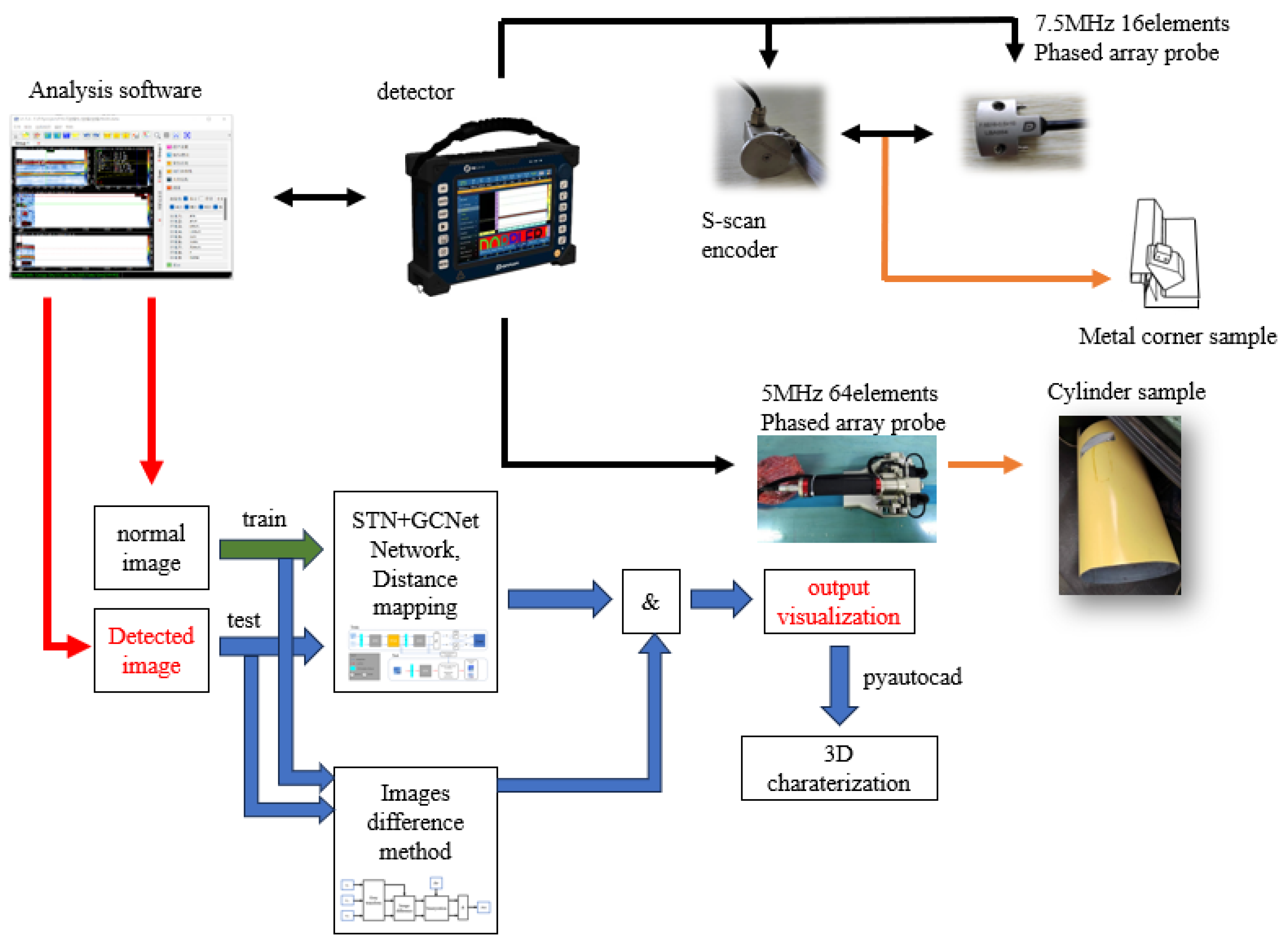
For non-destructive testing, it is urgent to develop a new intelligent testing technology based on fewer samples and no supervision. This paper takes anomaly detection as the starting point in order to solve the defect detection problem in the case of small samples, and to solve the problem of false detection in the phased array S-scan data, relying on an ultrasonic nondestructive testing self-focusing probe, wheel probe, and corresponding encoder (which is totally different from the encoder in the proposed network) to conduct scanning detection. Based on the contrast learning method, intelligent detection technology can solve the problem of defect images caused by few samples. The detection technology only needs to bring normal detection samples into training, without the corresponding defect samples. The contributions of this paper are as follows:

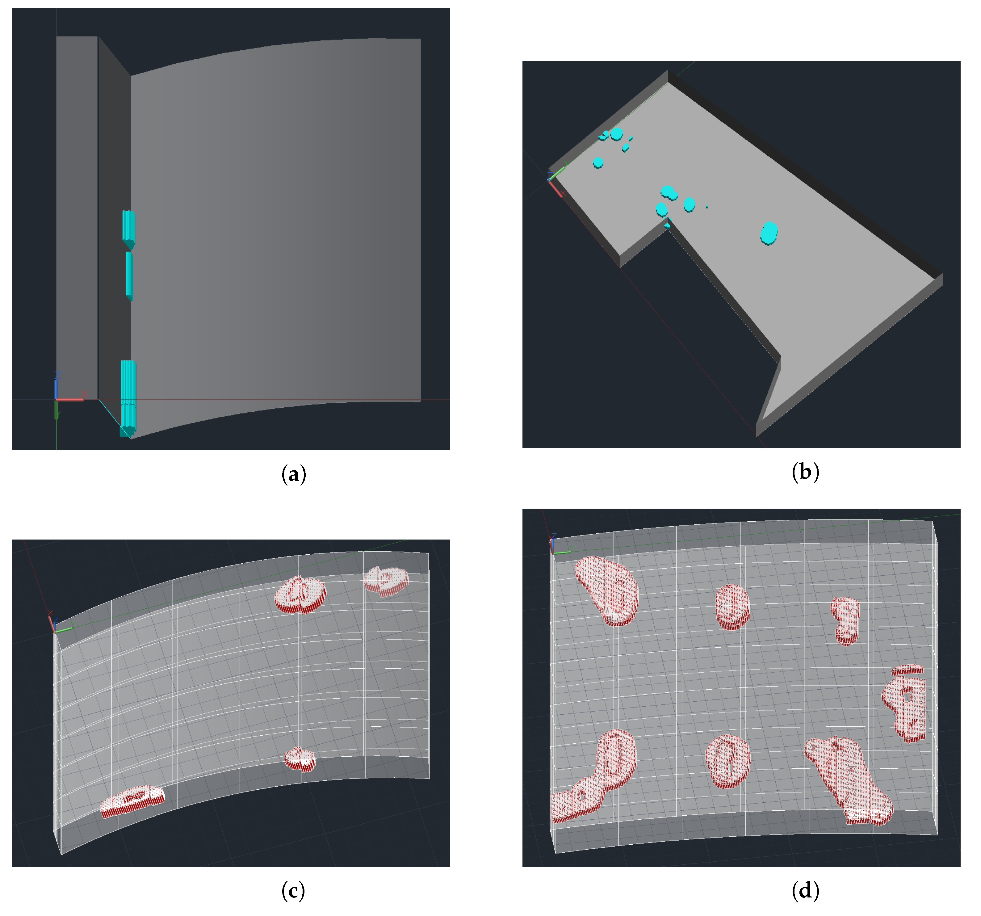
• This study realizes defect detection through the supervision of non-defect data with no output label. According to the detection results, three-dimensional defect characterization under several geometric structures is realized through the pyautocad module.
• A contrast learning strategy was adopted. The test image and homologous normal detection images under the corresponding detection modes (L-shaped structure or cylinder structure) were provided to obtain the positioning defects through Mahalanobis distance calculation.
• Two trainable CNN-based modules, STN and GCnet, were introduced to further enhance the detection and characterization effect of the whole method. The ablation experiment and performance comparison verified the necessity and rationality of the module structure.

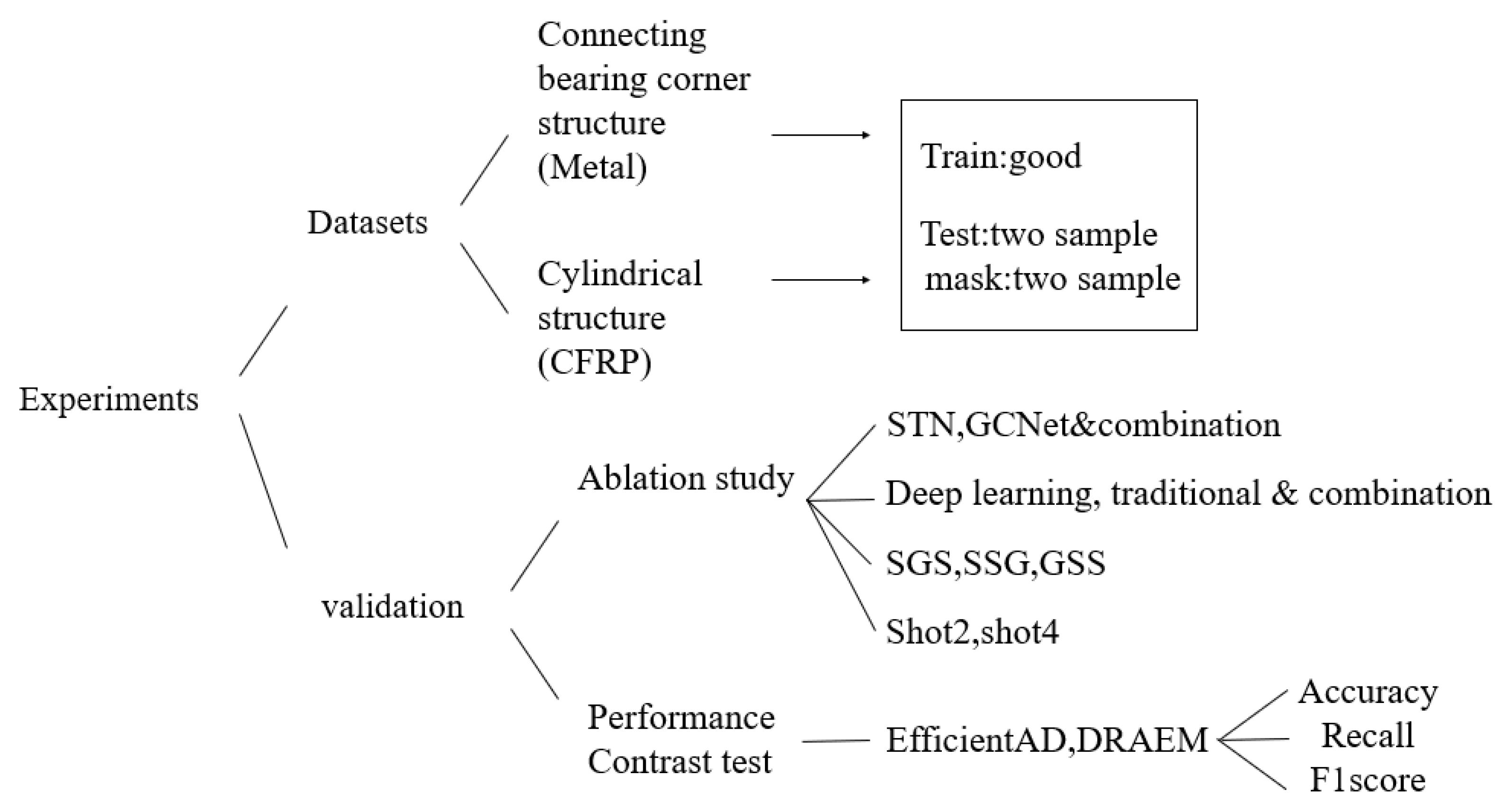
The rest of the paper is structured as follows: Section 2 summarizes the defect detection procedure and proposed method with STN and GCNet block based on PAUT. Section 3 introduces the experiments, including an ablation study, a performance comparison of four samples with three other state-of-the-art methods, and 3D characterization. Section 4 summarizes the research findings and offers future research directions.

2. Proposed Method

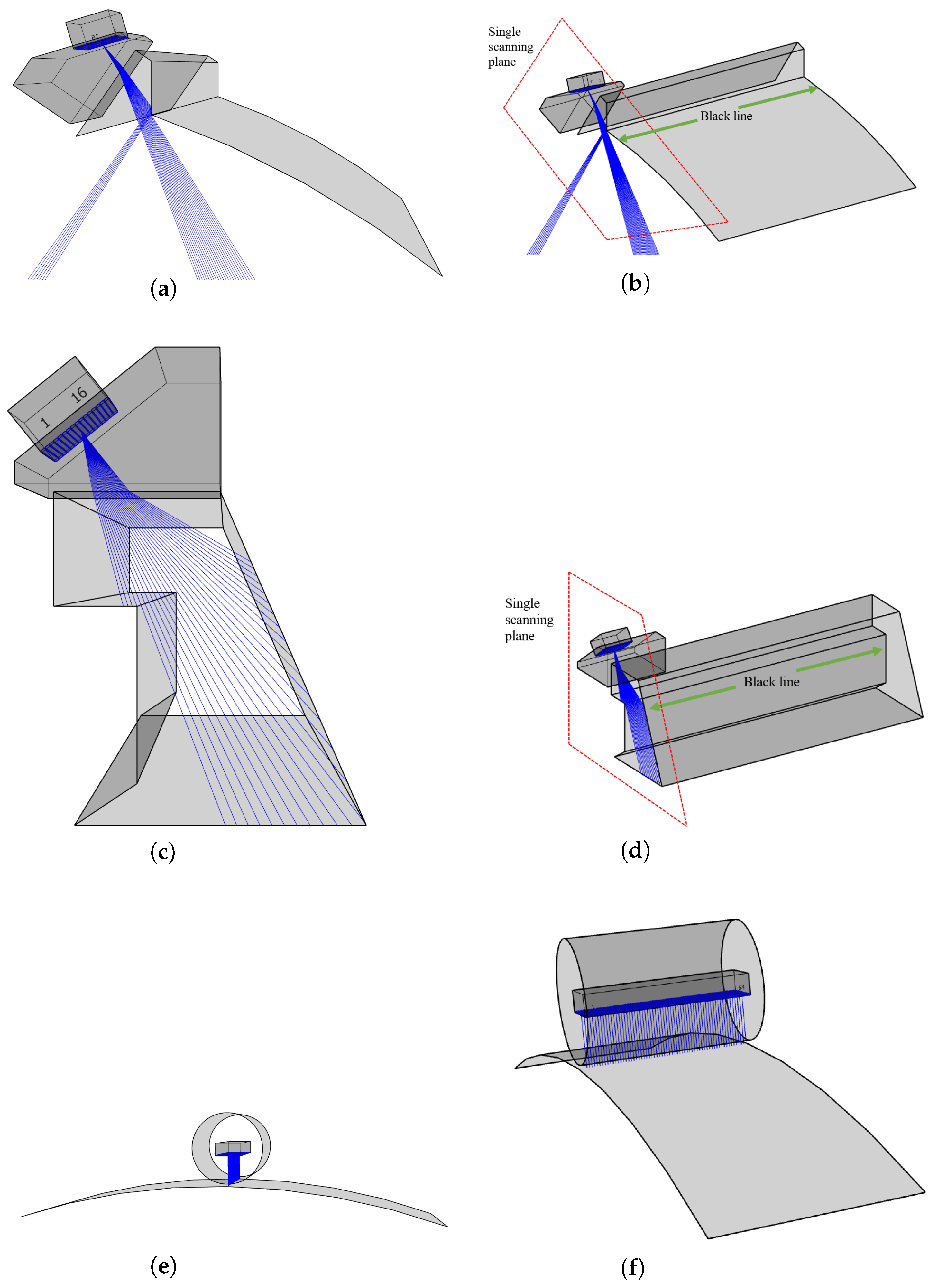
This research focuses on the defect detection and characterization of the L-shaped structure and cylinder structure. A program diagram in pseudo-code was created to clarify the defect detection process of this study. The pseudo-code was developed based on the network after training convergence, with an input of S-scan images corresponding to metal structure detection or C-scan images corresponding to CFRP detection; It represents the image to be detected. The output Ot was segregated into Ot1 for image difference output and Ot2 for Mahalanobis distance calculation based on contrast learning. Mid means the intermediate components in programs or mathematical operations. Mid5t means the final intermediate input by the test image, and then Mid5t is used for the distance calculation. In [B,C,H,W], B, C, H, and W represent the batch size, channel, height, and width of the variable. T relates to the transposition of one matrix. There are also some functions in the pseudo-code; difference(*), STN+GCNet(*), unfold(*), concat(*), fold(*), covariance(*), inverse matrix(*), and sqrt(*) represent the image difference method mentioned in the paper, intermediate characteristic quantity of the contrast learning network, tensor expansion operation, tensor concatenation operation, tensor folding operation, covariance matrix, inverse matrix, and root square value, respectively. The training of the corresponding network will be discussed further in relation to the contrast learning network. After the network is introduced, two improved CNN-based modules will be explained. Section 2.2 accounts for the distance map calculation, aimed at defect visualization. Section 3.4 will introduce the three-dimensional characterization. In the L-shaped structure task, the traditional method is used, while in the cylinder structure task, only the contrast learning network is used to extract the features for detection.

2.1. Feature Extraction Method

2.1.1. Dual-Normal Detection Image Difference Method

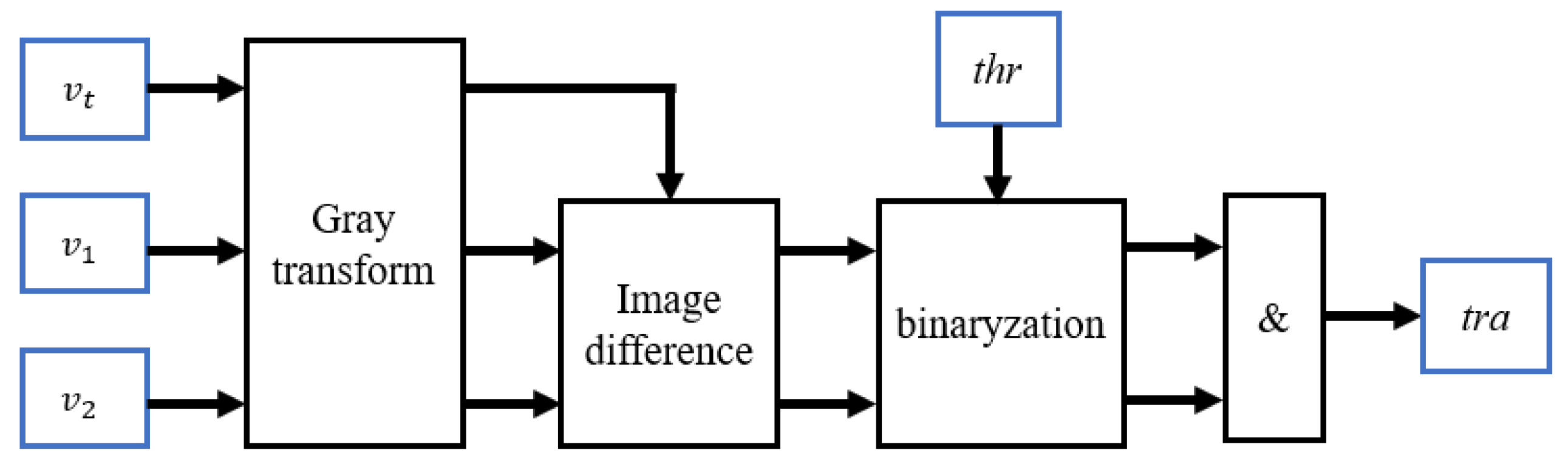
The simple and practical traditional method of defect detection should not be abandoned entirely. Traditional defect detection methods are introduced, including image difference and binarization processing. Three images are input, including two images with randomly selected normal testing results from normal ultrasonic detection datasets, and one image of ultrasonic data to be detected, and the image difference method is carried out after gray-scale transformation. While $tra0$, $tra$ is the output result, the mathematical expression of threshold processing is shown in Equation (1), and the dual-normal detection image processing method adopted in this study is shown in Equation (2). $thr$ is the threshold. v represents a kind of image. $v_1$ and $v_2$ are two randomly selected images of the normal state, and $v_t$ is the test image to be detected. After the image difference method, two feature tensors with the same dimensions as the image gray-scale transformation are output. The same threshold is set for binary processing. The output image is obtained by the Hadamard product of two image dimension variables. Figure 1 depicts this improved difference calculation process. In this paper, the traditional method is combined with the contrast learning network to improve the defect detection effect of the S-scan data, and only the contrast learning method is used for the cylinder structure.

$$tra0=max(0,min(1,v-thr\left)\right)$$

(1)

$$tra=max(0,min(1,|v_1-v_{\mathrm{t}}|-thr))+max(0,min(1,|v_2-v_{\mathrm{t}}|-thr))$$

(2)

2.1.2. Contrast Learning Network Method

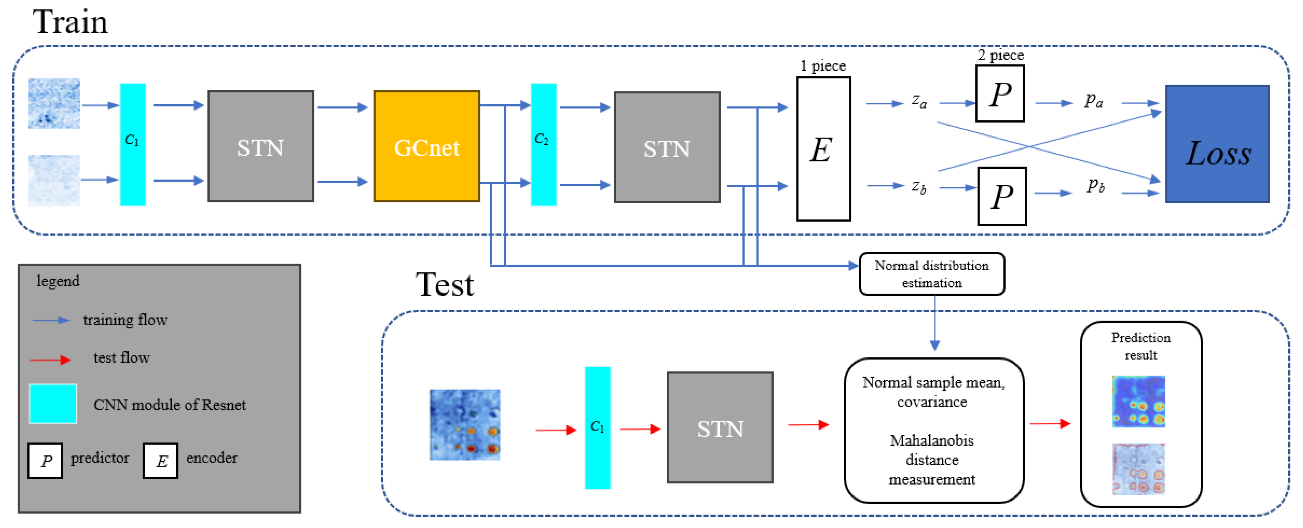
The normal sample’s common characteristics are identified through contrast learning. Accordingly, defects are located and detected by measuring the distance. Figure 2 illustrates the proposed network’s overall structure for contrast learning and distance map calculation. The purpose of establishing the contrast learning network is to utilize the pretraining network and the enhanced feature extraction ability of the network after the STN module and GCNet module. In Figure 2, the corresponding normal detection C-scan data of the plane plate are taken as the input and output legend, and the network relies on the Resnet18 pretrained structure. The last convolutional block in the original design of ResNet is removed, the STN module and GCNet module are incorporated into the pretrained Resnet18 structure, and the encoder and predictor are inserted into the tail end of the pretrained structure. The encoder is mainly composed of convolution, batch regularization, and relu modules, which are seen as one piece in Figure 2, and the encoder and predictor are composed of one and two pieces, respectively. The intermediate layer of batch regularization applied to the neural network replaces the dropout structure of the original pretrained structure and accelerates the training process. The dimensionality of the feature map is unchanged after passing through the encoder and predictor. The specific steps of data forwarding are as follows: the normal image set is input to the network in the form of random normal image pairs, and the network output is based on the function of cosine loss to make the network converge. There are some differences between network training and testing. After training, the network can retain the mapping synthesis feature information of normal samples, and a limited number of images that identify defects can be entered into the network to extract the abnormal features of the defects. Then, the defects can be located and segmented through distance graph calculation, as described in Section 2.2.

$$D(p_{\mathrm{a}},p_{\mathrm{b}})=\frac{p_{\mathrm{a}}}{\left|\right|p_{\mathrm{a}}\left|\right|}\frac{z_{\mathrm{b}}}{\left|\right|z_{\mathrm{b}}\left|\right|}$$

(3)

$$L=D(p_{\mathrm{a}},z_{\mathrm{b}})+D(p_{\mathrm{b}},z_{\mathrm{a}})$$

(4)

$z_a$ and $z_b$ are the output vectors of the encoder corresponding to the two input images, and $p_a$ and $p_b$ are the output vectors of the predictor head corresponding to the two input images. Cosine loss is calculated based on these vector features, as shown in Equation (4). Cosine loss, when formulated as given in Equation (3), has the distance measurement property, and the loss function established on this basis can make the network converge to form the ability to extract common features.

2.1.3. GCNet Block

GCNet is a convolutional network structure [25,26]. Due to the distance between the input and output dimensions, this structure can easily be combined with visual tasks to improve subjective and objective performance. This network structure combines the advantages of both SENet and NLNet. 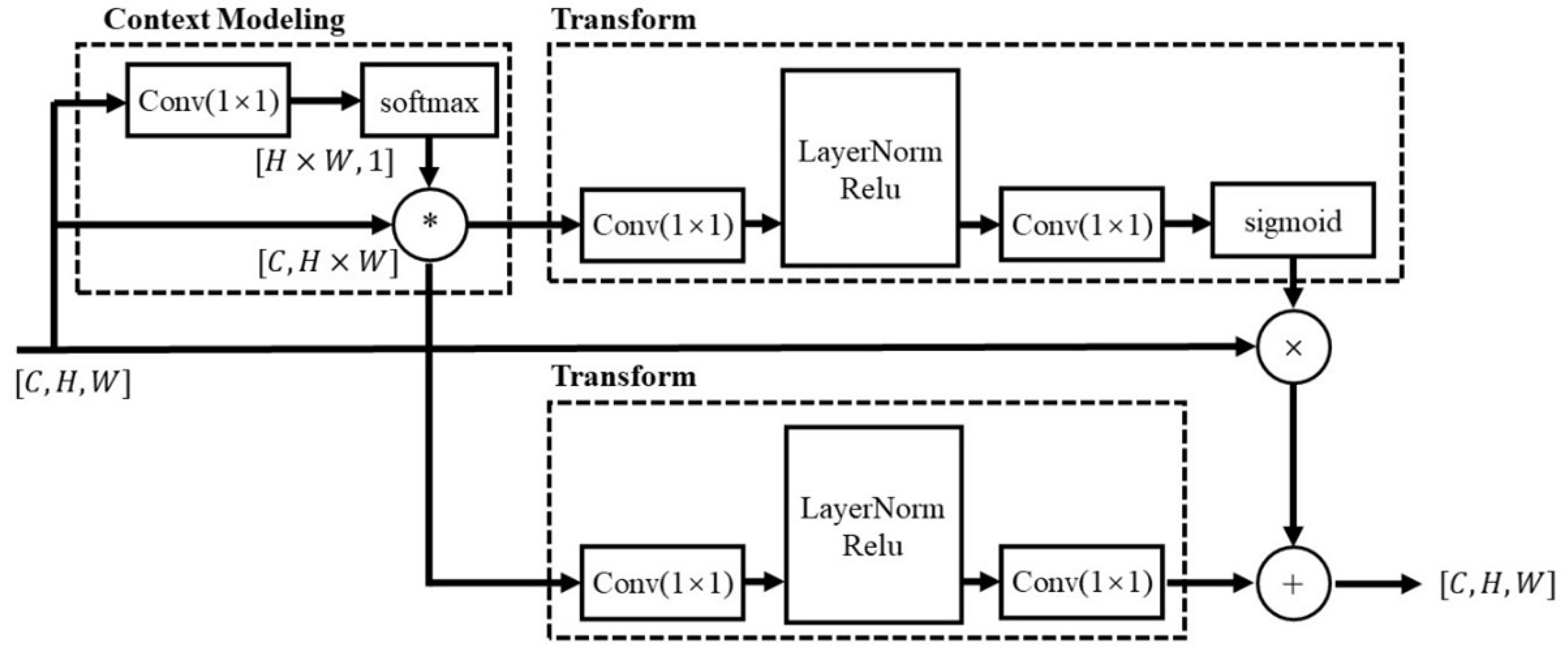It can not only use the global context modeling capability of NLNet [27], but can also be as lightweight as SENet [28]. In other words, the addition of GCNet will not hinder the training and testing of the original network structure. The dimension transformation relationship of the structure diagram and feature diagram is shown in Figure 3, which can be expressed by the mathematical relationship of Equations (5) and (6).

$$W_{\mathrm{con}}=\frac{exp\left(W_1{x}_{\mathrm{C},\mathrm{H},\mathrm{W}}\right)}{{\sum }_{k=i}^{h\times w}exp\left(W_i{x}_{\mathrm{C},\mathrm{H},\mathrm{W}}\right)}$$

(5)

$$output=W_{3}LN\left(W_2{W}_{\mathrm{con}}{x}_{\mathrm{C},\mathrm{H},\mathrm{W}}\right)$$

(6)

In Equation (6), $x_{\mathrm{C},\mathrm{H},\mathrm{W}}$ and $output$ represents the input and output of GCNet, respectively, $W_{\ast }{x}_{\mathrm{C},\mathrm{H},\mathrm{W}}$ is the $w_{\ast }$ convolution for $x_{\mathrm{C},\mathrm{H},\mathrm{W}}$, and $W_{\mathrm{con}}·x_{\mathrm{C},\mathrm{H},\mathrm{W}}$ represents the weight of the global attention pool. exp() relates to the exponential operation in the softmax calculation. $x_{\mathrm{C},\mathrm{H},\mathrm{W}}$ is reshaped to the tensor dimension by (C, H × W). After the synthesis by one output channel convolution of the input feature map, the tensor becomes (1, H × W). Then, the weight of each position in the (1, H × W) tensor is reflected through softmax, and the global attention weight is obtained by the matrix product with each channel input of the original input feature map. In other words, as shown by the output of context modeling in Figure 3, the weight of global attention mainly reflects the importance of the location, and the determination of defects in the S-scan detection data is also related to the channel characteristics of image data. The GCNet structure extracts channel characteristics through bottleneck transformation, that is, the ‘transform’ given in bold font in Figure 3. In Equation (5), $W_{3}LN\left(W_2\right)$, the bottleneck transformation is structurally similar to the autoencoder structure, and both of them have the same characteristics of small middle feature dimensions, the difference being that the dimension reduced by the bottleneck transformation is the channel dimension. In this study, two sets of bottleneck transforms are used and the sigmoid module is added to one of them. By reducing the convolution of feature map channels and the convolution of channel number reduction, a new feature map is obtained by dot multiplication and added to the original feature map. The feature map introduces the spatial channel feature information of the original feature map in a lightweight network way.

2.1.4. Spatial Transformer Network

The STN structure is based on affine transformation [29]. In terms of results, affine transformations have the same effect as common data augmentation, such as translation, scaling, rotation, and flipping. However, data augmentation focuses on the random transformation, which will boost the generalization performance in the training process. The affine transformation describes the image data transformation with a unified expression, which has a clear expression, and has the feasibility of integrating with the network structure compared with the data enhancement.

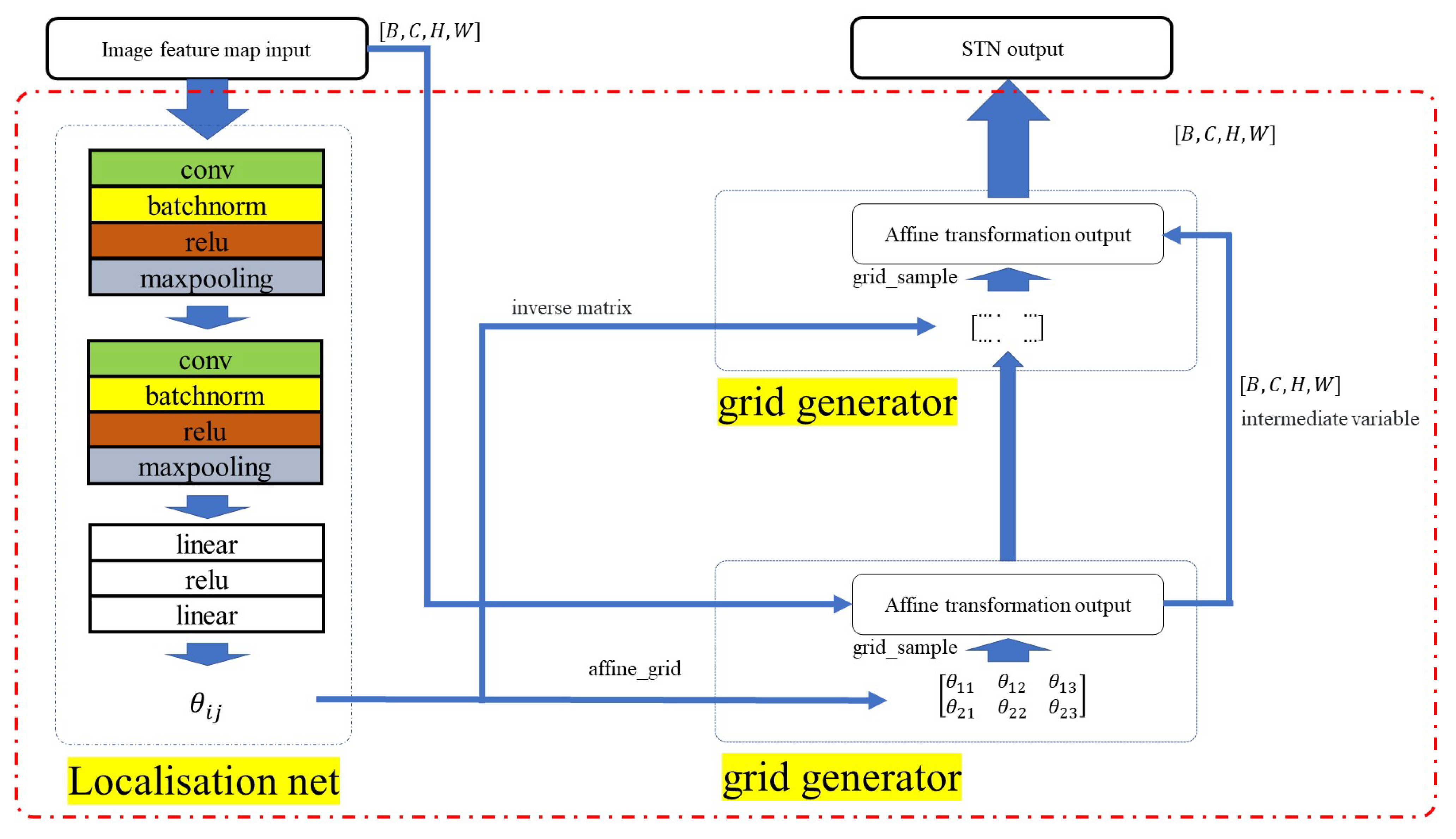
The STN structure introduces spatial geometric transformations such as translation, scaling, and rotation into the convolutional network structure. In this study, the introduction of the STN structure can better perceive the internal public features of input data, which is conducive to the natural wave extraction of S-scan detection data. The structure diagram of STN is shown in Figure 4. The specific structure of the network in the red box has something in common with GCNet: the consistency of the input and output dimensions. The structure in Figure 4 is divided into two parts according to the original paper [24]: the localization net and grid generator. The localization net consists of a trainable convolution network and linear connection layer, including batchnorm2d, relu and maxpooling layers and a linear connection layer. The linear connection layer consists of a linear layer and relu layer. The network outputs six parameters, set as ${\theta }_{\mathrm{ij}}$, which is connected to the grid generator. ${\theta }_{\mathrm{ij}}$ constructs the affine transformation matrix, referred to as a in Equation (7), according to affine transformation method. A and $A^{-1}$ depict the pixel value mapping process according to the affine transformation matrix a and $a^{-1}$. The pixel coordinate relationship corresponding to the affine transformation can be represented by Equations (8) and (9).

$$\left(\begin{array}{c}{x}_{\mathrm{i}}^t\\ y_{\mathrm{i}}^t\\ 1\end{array}\right)=\left(\begin{array}{ccc}{\theta }_{ij}& {\theta }_{ij}& {\theta }_{ij}\\ {\theta }_{ij}& {\theta }_{ij}& {\theta }_{ij}\end{array}\right)\left(\begin{array}{c}{x}_{\mathrm{i}}^s\\ y_{\mathrm{i}}^s\\ 1\end{array}\right)=a\left(\begin{array}{c}{x}_{\mathrm{i}}^s\\ y_{\mathrm{i}}^s\\ 1\end{array}\right)$$

(7)

$$image\left[(x_{\mathrm{i}}^{s1},y_{\mathrm{i}}^{s1})\right]=Aimage\left[(x_{\mathrm{i}}^t,y_{\mathrm{i}}^t)\right]$$

(8)

$$image\left[(x_{\mathrm{i}}^{s2},y_{\mathrm{i}}^{s2})\right]=A^{-1}image\left[(x_{\mathrm{i}}^{s1},y_{\mathrm{i}}^{s1})\right]$$

(9)

Equation (7) expresses the coordinate correspondence before and after the affine transformation of the image, that is, the pixel value of the original image before the affine transformation determines the pixel position according to its pixel position and the affine transformation matrix. ${\theta }_{11}$, ${\theta }_{12}$, ${\theta }_{21}$, and ${\theta }_{22}$ correspond to the image rotation transformation parameters in the affine transformation. ${\theta }_{13}$ and ${\theta }_{23}$ correspond to the image translation parameters, $x_{\mathrm{i}}^s,y_{\mathrm{i}}^s$ represent the transformed coordinates, and $x_{\mathrm{i}}^t,y_{\mathrm{i}}^t$ represent the coordinates before transformation.

According to the position correspondence relationship in the affine transformation represented by this affine transform matrix, bilinear interpolation is used to solve the decimal problem in the calculation of pixel coordinates, and on this basis, the pixel value filling of the image after affine transformation is completed. In order to retain the characteristics of the image and avoid the obvious discontinuity at the boundary after filling, the reflection filling is adopted. When interpolating the boundaries of an image feature tensor, it fills the edge values of the image or tensor into the extended region in a mirror image. The input of the grid generator at the second layer is composed of the inverse matrix of the affine transformation parameter matrix and the output image feature of the affine transformation at the first layer, and the pixel value after the second layer’s affine transform is filled in the same way. The final output of the STN module is provided by the second layer affine transform output image feature.

2.2. Defect Map Calculation

According to the defect-free normal detection image set composed of different normal images, considering the relatively small amount of data in the training stage and in order to reduce the loss of information in the network, two output points are set on the network. The feature map of the two output points is synthesized (10). The $synthesize$ function corresponds to lines 3 through 9 of the pseudo-code in Algorithm 1. The mean and covariance characteristic quantities are called the normal distribution parameters, and the distance we need is calculated using Equation (11).

Algorithm 1 Pseudocode for defect detection of PAUT using improved contrast learning

Input It(S-scan or C-scan data detected image) with shape [B,C,H,W],In(N normal images randomly selected by normal image set) with shape [B,C,H,W] Output Ot(An image of the same size as the input image) with shape [B,C,H,W],Ot1 produced by dual-normal detection images difference meth,Ot2 produced by deep learning network. 1: Ot1 = difference(It,In)                     ▹ only for L-shaped and inner structure 2: (xn and yn,xt and yt) = STN+GCNet(In,It) 3:   4: Mid1 (shape:[B,C1,H*W/(16*16)]) = unfold(x,kernel size=4,stride=4) 5: Mid1 reshape to Mid2(shape:[B,C2,C1/C2,H/16,W/16]) 6: y (shape:[B,Cy,H/16,W/16]) repeats C1/C2 times to Mid3    (shape:[B,Cy,C1/C2,H/16,W/16]) 7: Mid4 = concat(Mid2,Mid3) (Mid4 shape:[B,C3,C1/C2,H/16,W/16])    (Mid2(x),Mid3(y):synthesise two output points(xn and yn,xt and yt) by STN+GCNet) 8: Mid4 reshape to Mid5(Mid5 shape:[B,C3*C1/C2,H/16,W/16]) 9: Mid5 = fold(Mid4,kernelsize=4) and reshape to[B,C3,H*W/(4*4)] 10:   11: Mn = mean(${\sum }_{n=1}^N\mathbf{Mid}\mathbf{5}$) 12: for  $i=1$  to  $H\ast W$  do 13:       Cov[:,:,i] = Covariance(In1[:,:,i].T) 14: end 15: for  $i=1$  to  $H\ast W$  do 16:       Cov1[:,:,i] = Inverse matrix(Cov[:,:,i]) 17:       distance[i,:] = sqrt[(Mid5t-Mn[:,:,i]).T*Cov1[:,:,i]*(Mid5t-Mn[:,:,i])] 18: end 19: distance reshape to [B,H/4,W/4] interpolate to [B,H,W],Ot2

$$f_{\mathrm{mn}}=synthesize(x,y)$$

(10)

$$D=\sqrt{{(f_{\mathrm{mn}}-{\mu }_{\mathrm{mn}})}^T{\sum }_{mn}(f_{\mathrm{mn}}-{\mu }_{\mathrm{mn}})}$$

(11)

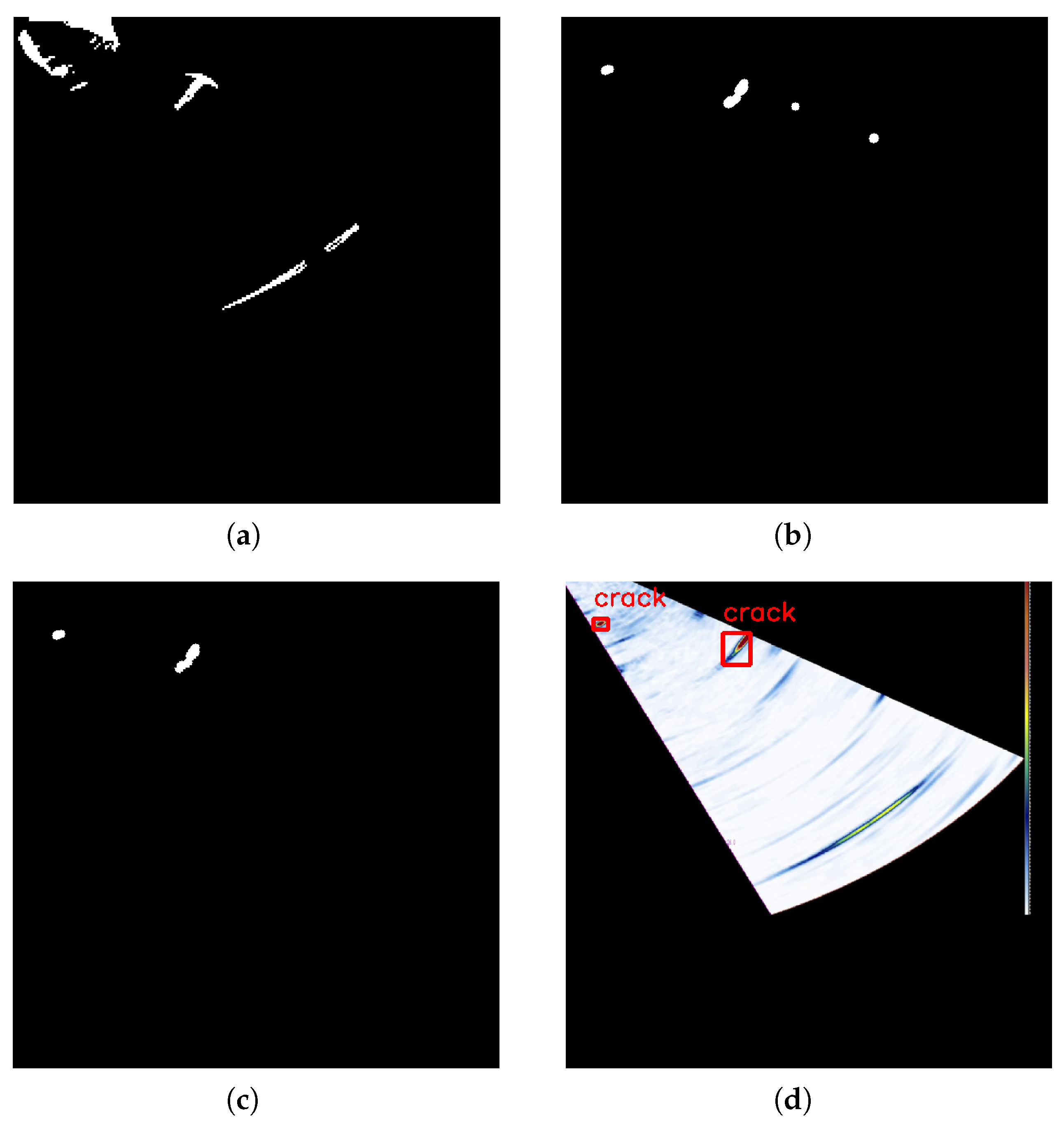
In Equation (10), T represents the transpose, $f_{\mathrm{mn}}$ represents the feature vector after the image passes through the network, ${\mu }_{\mathrm{mn}}$ is the mean value of the vector, and the subscript m,n maps the corresponding position of the original size map. $\sum _{mn}$ is the corresponding covariance matrix. The mean and covariance values provided relate to the computation of the mean and covariance shown in the latter portion, from line 11 to line 19 in pseudo-code Algorithm 1. The diagonal element of the covariance image matrix represents the difference between pixel values and at corresponding positions of the input image, and the non-diagonal element represents the correlation between different pixel values. Therefore, it can be seen that the average value and covariance feature map can represent the main features of the images in the normal detection image set without defects. According to the network loss function, the feature quantity between the normal detection images is relatively close. When the abnormal detection image is input into the network, the vector data with large difference from the normal feature quantity will be obtained at the two output points, that is, the abnormal detection image will be far away from the normal distribution of the normal distribution parameters at the corresponding position of the defect. In this paper, Mahalanobis distance is applied to calculate the image point by point, and the threshold processing is used to help locate the defects. D represents the defect’s distance measurement, which measures the possibility between defect or normal situation, and Mahalanobis distance is calculated according to Equation (9). The larger the D value of a certain position, the higher probability of defects exists at that position.

3. Experiments

3.1. Settings of Phased Array Ultrasonic Testing and Deep Learning

In this paper, the geometric structure of two typical materials is used as the basis of verification in the proposed method. The cylinder structure sample of carbon fiber composite material and two L-shaped structure samples of metal hanger bearing force are detected. The detection diagram is shown as the upper part of Figure 5. For the detection of couplings, distilled water and CG-98 flaw coupling agent are used for carbon fiber composite materials and metal structures, and the ultrasonic detection gain is 10 db and 35 db, respectively. Local gain methods such as DAC and TCG are not used. The two metal L-shaped structures used in the experiment are called the corner structure and inner structure. The S-scan angle of the corner structure is from 26 degrees to 60 degrees, and the S-scan angle of the inner structure is from 23 degrees to 75 degrees. The wheel probe’s C-scan gate is set from 1.3 mm to 3 mm.

The metal L-shaped structure detection data are completed by using a 7.5 MHz self-focusing shear wave probe with 16 array elements and a 24 step/mm scanning encoder (obtaining the distance by electric pulse counting, which differs from the network encoder mentioned above). The cylinder structure detection data are completed by single-line scanning with a 5 MHz longitudinal wave wheel probe with 64 array elements. A Doppler PhanscanII portable detector is used in this study for detection and to import data through its software. Since the two kinds of detection have different data formats, there are further different characterization traditional processing methods to decide the defect length of the L-shaped structure and the cylinder structure. We design the detection method and successfully detect several defects, as described in the next part. The overall detection can be summarized in Figure 5.

The Doppler analysis software can restore the setting state information during ultrasonic detection, mainly displaying the S-scan and C-scan. The red line represents the output of normal data from the analysis software for subsequent training, and the test data are output from the analysis software to enter the contrast learning model and dual image difference module, finally becoming the detection results. The green arrow signifies the network’s training phase. The network can only be tested after training. The ampersand symbol represents the operation of the output of both methods.

The detection beam transmission map is shown in Figure 6. In the cylinder structure, the two samples are basically consistent in shape, detection setting, and principle, so they are unified as a schematic diagram in Figure 6e,f. Considering the characterization of defects using the −6 db method and further performance improvement, for the traditional image difference method, the threshold should exceed 128 and be set to 150.

The implementation of deep learning consists of software and hardware. The hardware part adopts a GTX 1080 Ti with 11 GB video memory, and the software part adopts the pytorch framework (1.10.0 version). The SGD optimizer with a learning rate of 0.0001 and momentum of 0.9 is used in the proposed contrast network. The dataset consists of an unsupervised learning part and a defect depth dataset with a supervised learning label. The detection data of the flatten panel is considered to be easier to obtain due to the type and cost of the probe. Hence, the unsupervised comparative learning part is composed of the S-scan dataset of the L-shaped structure and the C-scan detection dataset of the panel part. The dataset of the metal L-shaped structure and the dataset of the panel part include 90 normal ultrasonic S-scan images and 90 normal ultrasonic C-scan images, respectively. The dataset structure is shown in Figure 7. The cylinder structure uses the flatten panel’s ultrasonic detection data for training.

3.2. Ablation Study

The detection of corner structures is more difficult, and the identification effect of different methods or fine-tuning within methods cause significant differences, so we use the corner structure as the base of the ablation study. The ablation experiment is divided into two parts. One part consists of switching the network structure sequence. GSS, SGS, and SSG, respectively, represent the combination sequence of three different modules to form the network structure. The comparison results, which are related to the mean value of the F1 score and other indicators, are shown by two-shot normal images and four-shot normal images for three network structures in

Table 1. Ablation study for the corner structure.

Method	Shot Num	Only GCNet	Only STN	Combination
shot 2	precision	0.1123	0.1510	0.2023
	recall	0.9311	0.7726	0.9329
	F1 score	0.2005	0.2513	0.3326
shot 4	precision	0.1438	0.1229	0.2167
	recall	0.9315	0.8399	0.4440
	F1 score	0.2492	0.2145	0.2912

. SGS is the structure of STN + GCNet + STN. The ablation experiment should not be limited to the improvement of objective indicators, and the effect of the model should also be reflected in the visual subjective evaluation. The other part of the ablation experiment is the result of the separate test of the traditional structure and the deep learning network structure. The detection and recognition effect of this method is further observed. Only the deep learning structure, traditional structure, and combination result are shown in Figure 8. Obviously, only after the combination of the two methods is there a better recognition and detection effect.

3.3. Performance Contrast Study

The performance mainly includes the model performance parameter, represented by the F1 score, IOU, and training time. The training time corresponds to the efficiency of introducing one method in industrial solution, and has been tested in the experiments. Additionally, the F1 score can combine accuracy and recall rate as a comprehensive indicator of network performance.

The DRAEM anomaly detection method, the best performing method, in comparison to the methods presented in this paper, takes the least time, requiring 2 min for cylinder surface detection training. The detection performance is compared with three methods with excellent performance in the field of anomaly detection: reverse distillation, DRAEM, and EfficientAD. The comparison methods are based on the S-scan of metal structures corresponding to Figure 9 and Figure 10 and the C-scan of cylinder structures, which is related to Figure 11. From these three sets of comparison results, it can be seen that neither DRAEM nor EfficientAD methods have a good detection ability for PAUT data, and the visualization effect is not good. The EfficientAD method divides a large number of non-defect data points into defects. The number of missed defects in DRAEM is three, which is similar to that of the proposed method, but it can be seen from the detection image that it is greatly affected by the noise of ultrasonic data, and false detection is generated at the edge of the dataset. The training time of the proposed method is 7 min over a few epochs to obtain a better performance, and the number of missed defects in the proposed method is 0. The F1 score in

Table 2. Performance comparison in CFRP cylinder structure.

Method	Sample	Precision	Recall	F1 Score	IOU
Reverse distillation	sample1	0.0058	0.5151	0.0115	0.0058
	sample2	0.0294	0.4943	0.0555	0.0295
EfficientAD	sample1	0.0250	0.6545	0.0483	0.2486
	sample2	0.0481	0.6587	0.0898	0.0472
SSG	sample1	0.0530	0.3071	0.2154	0.0475
	sample2	0.1554	0.3509	0.0898	0.1217
DRAEM	sample1	0.0688	0.7584	0.1261	0.0680
	sample2	0.1719	0.8531	0.2861	0.1702
SGS	sample1	0.0936	0.4300	0.1536	0.0837
	sample2	0.1902	0.8215	0.3089	0.1848

and

Table 3. Performance comparison of metal corner structure.

Method	Sample	Precision	Recall	F1 Score	IOU
Reverse distillation	inner	0.0623	0.7920	0.1155	0.0630
	corner	0.1229	0.9065	0.2165	0.1309
EfficientAD	inner	0.0707	0.5561	0.1255	0.0832
	corner	0.2134	0.1635	0.1842	0.1275
DRAEM	inner	0.0128	0.3026	0.0245	0.0475
	corner	0.1236	0.4809	0.1863	0.1023
SGS	inner	0.1719	0.8531	0.2861	0.1702
	corner	0.1651	0.9754	0.2835	0.1783

also indirectly shows how good the model is. As can be seen from the comprehensive performance index F1 score of the model, the structure implemented by the SGS network combination in this model has the best performance in terms of the test results, while the DRAEM method is inferior to the SGS model but exceeds the performance parameters of the SSG model. The effect and training time of the reverse distillation method and EfficentAD method are similar. In summary, the advantages of this method are illustrated from both subjective and objective perspectives.

3.4. 3D Defect Characterization by Pyautocad

Autocad is more common in modeling related tasks, and its file format is used to realize assisted defect identification in phased array ultrasonic imaging. Acoustic analysis software such as CIVA [30] and Beamtool [31] can adopt the same model file format. In this study, 3D characterization was achieved by using autocad and the detection results of the proposed method. Using the pyautocad interface on python IDE, the coordinate index of the defect location can be obtained from the detection result of the binary image format, and then the 3D structure of the defect can be constructed with the micro cylinder using the pyautocad command. An additional cylinder plate with an unidentified flaw is used in three-dimensional characterization, and the results of the analysis can be seen in Figure 12c. For a cylinder structure with fixed curvature, the inclination angles of defects at different positions are calculated directly according to simple angle relations. The characterization model shown in Figure 12 obviously and intuitively reflects the specific defect forms presented by the detection results of the proposed method.

4. Discussion and Conclusions

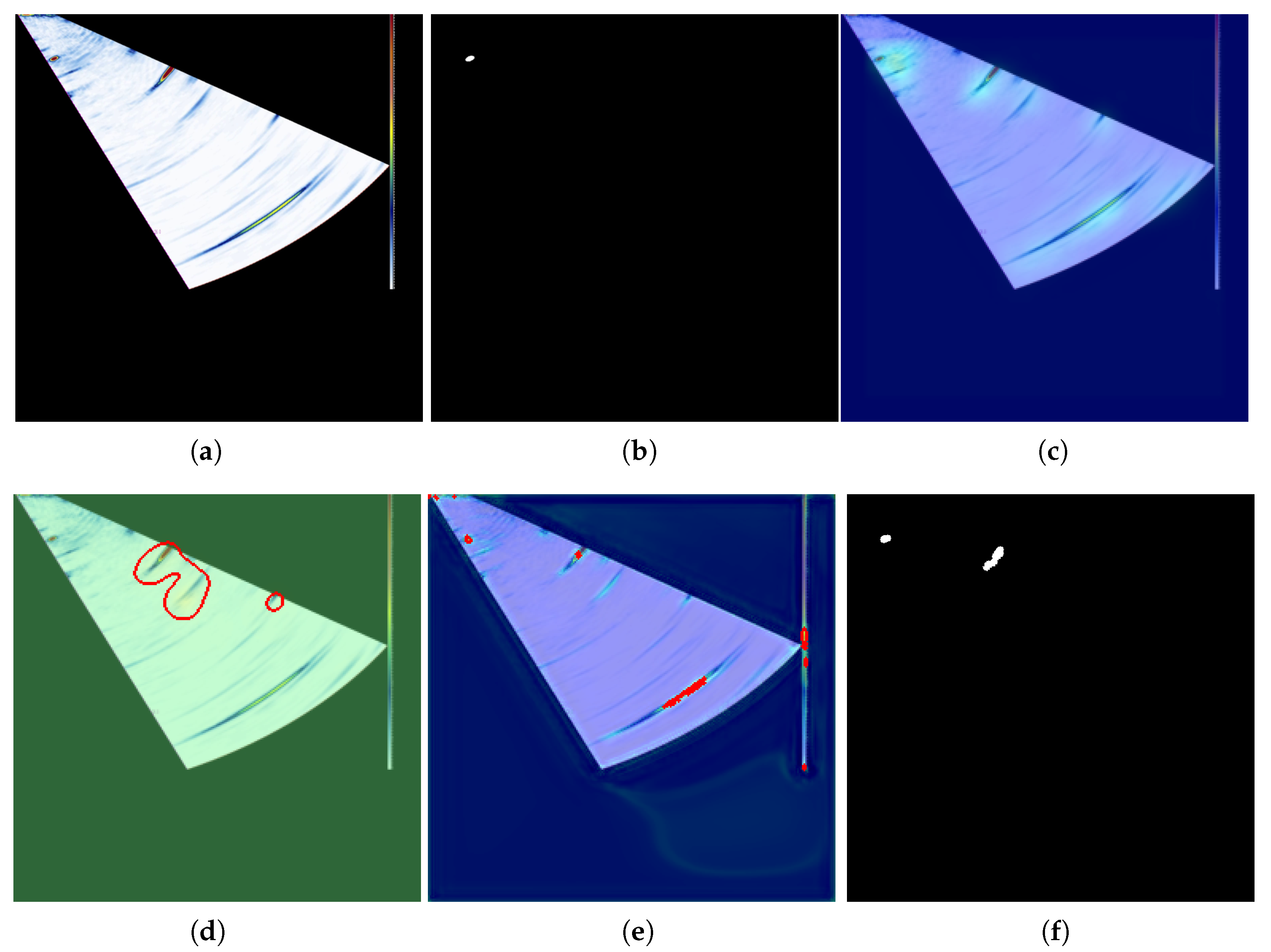
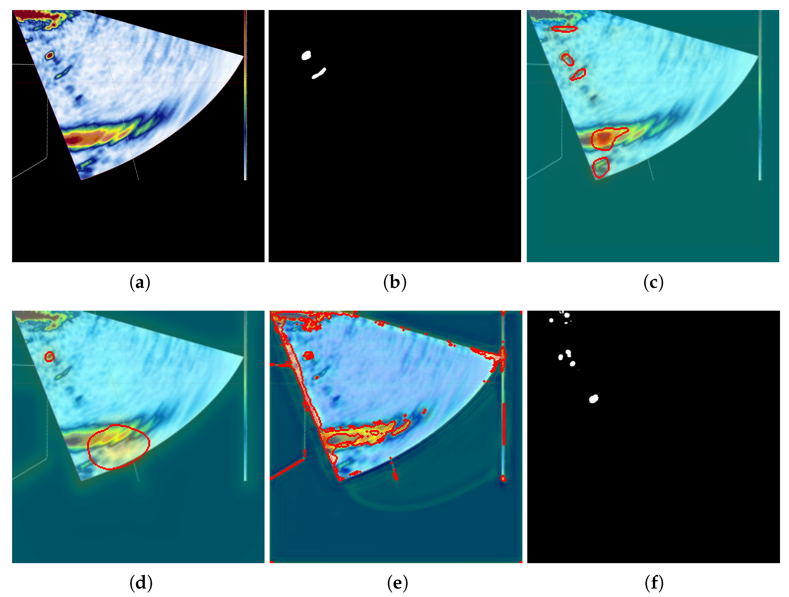
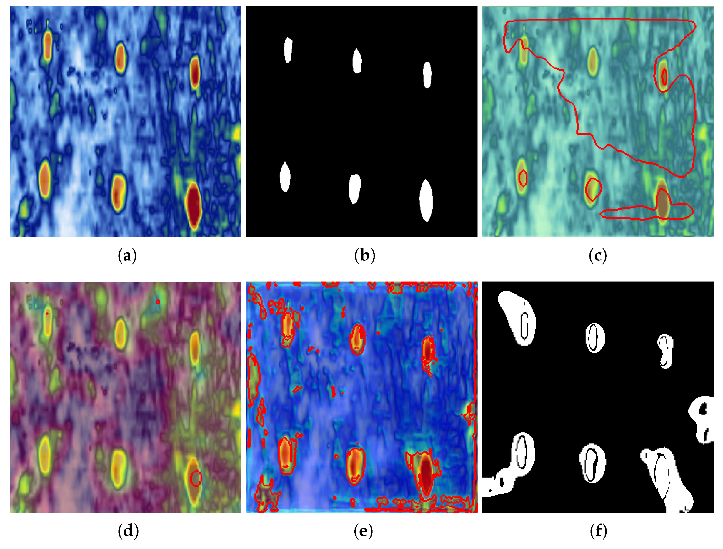
In this paper, two common aircraft structures, namely the CFRP cylinder plate and metal corner bearing structure, are studied using ultrasonic detection result recognition. The contrast learning model with pretrained weights is applied to the defect identification of ultrasonic detection data, and the STN and GCNet structures are used to further enhance the feature extraction ability. In the actual phased array ultrasonic detection process, the defect judgment of the phased array S-scan data image usually only focuses on the specified area. For example, within a certain gate range, as long as the echo occurs at a specified position within the gate range, it can be identified as a defect. This method is applied to a new sample, based on finished acoustic analysis. However, this method focuses on covering the global scope of the S-scan image in the absence of acoustic analysis. Any anomalies in the range of the S-scan image will be identified as defects. This method only needs to detect the image normally to provide the structure’s natural wave information, and the size and range of the natural wave usually fluctuate during the scanning process, so it is difficult to determine the defects through a simple image difference method. The experimental results show that the combination of the image difference method and contrast learning model is more suitable than using only one method to solve the problem of the difficult identification of S-scan image defects, and has surpassed some state-of-the-art methods in the AD field. On the basis of the wheel probe, the data format of surface plate defect identification is not vastly different from that of the panel parts, and can be identified directly through the contrast learning network. There are also some limitations of the work presented in this paper. More threshold processing is used in the testing process, which is unfavorable for the overall generalization performance of the method.